Article

Locating Battery Swapping Stations for a Smart e-Bus System

1
School of Industrial Management Engineering, Korea University, Seoul 02841, Korea
2
Logistics System Research Team, Korea Railroad Research Institute, Uiwang 16105, Korea
3
Graduate School of Logistics, Incheon National University, Incheon 22012, Korea
*
Authors to whom correspondence should be addressed.
Sustainability 2020, 12(3), 1142; https://doi.org/10.3390/su12031142
Submission received: 15 December 2019 / Revised: 28 January 2020 / Accepted: 30 January 2020 / Published: 5 February 2020

Abstract

:
With the growing interest and popularity of electric vehicles (EVs), the electrification of buses has been progressing recently. To achieve the seamless operation of electric buses (e-Buses) for public transportation, some bus stations should play the role of battery swapping station due to the limited travel range of e-Buses. In this study, we consider the problem of locating battery swapping stations for e-Buses on a passenger bus traffic network. For this purpose, we propose three integer programming models (set-covering-based model, flow-based model and path-based model) to model the problem of minimizing the number of stations needed. The models are applied and tested on the current bus routes in the Seoul metropolitan area of South Korea.

1. Introduction

As the concern over global warming and energy issues grows, electric vehicles are increasingly considered as an alternative to traditional vehicles and have hence gained much attention from the general public. With the increasing interest and popularity of electric vehicles (EVs), many countries have developed electric buses and introduced them on a trial basis. In South Korea, the Seoul metropolitan government has operated electric buses around significant tourist destinations and has been gradually expanding the network [1]. Jeju island, the largest island in Korea, is preparing for pilot electric bus operation [2]. In addition to these attempts, academic research into the usefulness and operation policies of electric vehicles is actively underway [3]. Outside Korea, China has grown its market size of electric buses significantly [4], and we can infer that the demand for e-Buses is increasing continuously. Other major countries, such as the U.S, European countries, and India, have trends of increasing demand and application of electric buses, and these trends are expected to continue in the future [5].
There are several types of electric buses, as well as operation methods. The most typical ones are the plug-in type, the wireless rechargeable type, the trolley bus and the battery exchange type. Since each method has its special characteristics, it cannot be easily concluded which is the best. However, depending on the type of electric bus, the factors and problems requiring consideration vary widely. For example, the trolley bus needs wires for electric supply. Thus the constraint of wires becomes an important consideration, and there are many studies treating issues related to wire networks. Teoh et al. [6] cover routing network design and fleet planning for Malaysia’s transportation situation. On the other hand, for the battery charging system, efficient route configuration within a given battery capacity is important since charging takes time and is usually only possible in depots. Thus, regarding charging system problems, locating a depot or optimizing time scheduling given a network configuration are major concerns. In fact, some studies have focused on electric bus operations and the problem of locating charging stations. Relatively recently, Rogge et al. [7] aimed to optimize the charging schedule of electric buses to minimize overall costs, including vehicle investment, charger investment, operational costs, and energy expenses. Liu and Wang [8] treated the problem of locating several types of recharging facilities, especially wireless recharging facilities. There is also ongoing research into operating electric buses based on battery swapping. In battery swapping cases, each vehicle travels with a battery and can swap the battery at the designated places for exchange, so-called battery swapping stations. The advantage of the battery swapping system is that it does not require huge infrastructure as a trolleybus system does, and unlike the battery charging system, it is possible to replace the battery quickly along the route. In the battery swapping system, locating battery swapping stations is a crucial problem. Ko and Shim [9] deal with the issue of selecting the location of battery exchange stations for the seamless operation of electric taxis, which operate with no fixed routes. Furthermore, several studies deal with the issues related to the scheduling of battery swapping when operating electric vehicles or buses. For example, Chao and Xiaohong [10] and Kang et al. [11] dealt with the time scheduling problem of battery swapping systems. Sarker et al. [12] proposed a numerical model for selecting the location of battery swapping stations in terms of the supply of and demand for electricity, and the scheduling of electrical supply. Our paper differs from those studies in that we aim to determine both the location of swapping stations and the scheduling of battery swapping. We approach battery swapping systems as being underlying problem situations. In doing so, we deal with the problem of operating an electric bus in a public transit network with a battery swapping system. To achieve this, we assume the installation of a so-called Quick Charger Machine (QCM) over the public bus transit network (see Figure 1). We refer those who are interested in the QCM, to the web page of reference [13].
As Figure 1 shows, QCM is a machine installed in a proper bus station and it transforms an eligible bus station into a battery swapping station. Since the automated machine replaces the battery, it is possible to replace the battery within a short time (say, within one minute) while passengers are transferring. Inevitably, for the seamless operation of electric buses (e-Buses) in public transportation, some existing bus stations should play the role of battery swapping stations due to the limited travel range of e-Buses. Considering that the number of QCMs is related to the operational cost of the system, it is important to minimize the total number of QCMs installed. In this problem, we do not explicitly consider the installation costs of these QCMs, which may differ by location.
This problem can be partly viewed as a location routing problem (LRP) variant.The LRP considers vehicle routing and related resources (e.g., facilities, customers and so on) to find proper facility locations, determine the optimal number of facilities or vehicles, and optimize the routing plan [14]. The LRP itself has many variants depending on the particular purpose or problem situation [15,16]. In this paper, the problem is to find the number of facilities and their optimal locations. In the general LRP, some nodes have demands, and vehicles route them to satisfy those demands. In this problem, we can see the similarity with the LRP in the sense that the facilities considered are bus stations with a QCM and the vehicles travel over the bus transit network while preventing battery shortage by visiting some of the QCMs. There are many papers in literature (e.g., [17,18,19]) introducing the basic concept of the LRP, its variants and solution approaches. Amaya et al. [20] study the operation of vehicles and the location of depots with capacitated vehicles, a problem defined as the capacitated arc routing problem (CARP). The specific problem of that paper is that the service vehicle (SV) travels service arcs in a graph, and since the SV has a finite capacity, to enable its continuous service, it is replenished by a refilling vehicle (RV). There is a depot to refill the RV, and the paper tries to find the optimal location of the depot and optimal min-cost path. If we assume the refilling vehicles are fixed and uncapacitated, this problem situation becomes similar to our assumed problem situation. Nevertheless, our paper is completely different in that it considers the cost incurred in routing. Xing et al. [21] consider several depots in the CARP model. Bektaş and Elmastaş [22] deal with a similar problem to ours, and find the optimal locations for the depots, but consider just one main depot in the bus route for fulfilling buses without any other refill point. Yang and Sun [23] assume the problem of delivering goods to customers from a depot using electric vehicles. The depot serves as both a supply of goods and a battery swapping station. Within this setting, they select depot locations that minimize overall shipping costs. Rogge et al. [7] propose optimal charging priority and charging location in the battery swapping problem, and examine a similar situation to ours. However, this paper is different to ours in that it deals with a centralized charging system, which means that battery charging occurs only at the depot. Boccia et al. [24] deal with an interesting problem similar to ours in some respects. They determine the location of the facility on the flow network that maximizes the flow through the facilities. To summarize the above, our study significantly differs from previous studies. In our problem, each node (i.e., a bus station with QCM) can serve as a refill point while most of the previous works set a separate depot as the central refill point.
This paper is organized as follows. Section 2 presents the three different proposed mathematical programming models for the concomitant model. In Section 3, the proposed models are applied and tested on the current bus transit network in the Seoul metropolitan area of South Korea and the experimental results are discussed, including comparisons of the models. Finally, we provide a conclusion in Section 4.

2. Model

In this section, we present the mathematical programming models for swapping station deployments for an e-Bus transit network. The deployment of a network of swapping stations is essential given e-Buses’ limited travel range. This paper considers the problem of locating battery swapping stations for electric buses on a bus transit network while appropriately addressing the battery capacity of each bus in operation. Given the situation, the objective of our problem is to optimize network performance. Specifically, we maximize the flow covered by a predetermined number of stations or minimize the number of stations needed to cover traffic flows. For this, three different mixed-integer programming models are proposed to address the concomitant problem. These are the set-covering-based model (Section 2.3.1), the flow-based model (Section 2.3.2), and the path-based model (Section 2.3.3).

2.1. Assumption

Before presenting the mathematical models, we first present the assumptions while maintaining the essence of the problem. We note that all these assumptions are applied to the three models. First, battery swapping can be achieved within the time period the passengers are transferring so that the problem of interest is free from battery swapping time constraints. Second, if a bus route from a depot to the end does not require battery swapping during a journey, we exclude this route from consideration. Third, we also assume that a battery in the swapping station is always a fully charged battery; in other words, there are no replacements with an incompletely charged battery. Lastly, considering QCM assumptions, we ignore the possibility that there exist some stations where battery swapping facilities cannot be installed due to geographical and spatial problems or administrative problems.

2.2. Notation

The sets, parameters, and decision variables used in the models are listed in Table 1:
We remark that the eligibility of each bus stop for a QCM ( N s ) can be confirmed during the preprocessing process by considering factors such as electrical grid infrastructure and the availability of the construction space required for a QCM.

2.3. Mathematical Programming Formulations

In this section, we present the mathematical programming formulations for the problem of interest—i.e., set-covering formulation, flow-based formulation and path-based formulation—and then discuss the pros and cons of each formulation.In fact, we propose three types of formulations for the same strategic decision making problem of locating QCMs in a bus transit network. We will see that the set-covering formulation is efficient in terms of computational performance but that it lacks flexibility when incorporating additional issues such as Quality of Service. To address this drawback, flow-based and path-based formulations are also proposed since their models can incorporate these additional issues, as we will discuss in the subsequent sections.

2.3.1. Set-Covering Formulation

First, with the maximal ordered subset (MOS) defined in Table 1, this problem can be basically viewed as a set-covering problem. Figure 2 illustrates the definition of MOS and the basic idea of the set-covering formulation. If at least one QCM is included in all the MOSs for each bus route, we can confirm that no full battery discharge occurs during the bus’s traversal of that route, since MOS is defined as the maximal distance that an e-Bus can drive without needing a battery swap. By incorporating the definition of MOSs, the following formulation can be proposed to minimize the overall number of QCMs.
Model (Set-covering model)
minimize α N s y α
subject to β T α r N s y β 1 , r R , α N s r
y α = 1 , α D o
y α { 0 , 1 } , α N s
The objective function in Equation (1a) is to minimize the total number of QCM installations over the e-Bus transit network. We note that, as for conventional facility location models, this objective function can be easily modified to minimize QCM installations and annual maintenance costs. However, in this paper we limit our attention to minimizing the total number of QCM installations. Constraint () indicates that each MOS must contain at least one QCM, as discussed above. Constraint () guarantees that all the depots have QCM functionality.
We assume that | N s | is large enough to warrant that T α r N s ϕ for all r R , α N s r ; otherwise, the problem becomes infeasible. This formulation has a compact form, compared with the other formulations below. However, the set-covering model only suggests the locations of QCMs among potential bus station candidates for QCM installation with y variables. We will see that the other proposed formulations simultaneously determine not only the QCM locations but also the battery swapping schedule of each bus en route. Thus, with this formulation, it is difficult to take Quality of Service (QoS) into account because of the difficulty of analyzing the operational efficiency of each bus and route due to limited information on where and how many times battery swapping occurs. We discuss this aspect further in Section 3.5. The formulations introduced below complement these perspectives and should be more informative.

2.3.2. Flow-Based Formulation

As noted earlier, the set-covering formulation in Section 2.3.1 does not explicitly provide detailed locations of where to swap batteries for each bus (i.e., battery swapping scheduling for each bus en route). Thus, we here suggest an alternative model which overcomes the limitation of the first model. This model is based on the idea of minimizing the number of QCM installations while satisfying all the in- and out-flows and the connectivity of all stations. For this, we first introduce the additional notations in Table 2 and then introduce the flow-based model.
Model (Flow-based model)
minimize α N s y α
subject to x α κ r y α , α , κ N s with α r κ , r R
x α κ r y κ , α , κ N s with α r κ , r R
κ O r ( α ) x α κ r - κ I r ( α ) x κ α r = b α , α , κ N s with α r κ , r R where b α = 1 if α D o , b α = - 1 if α D d , and 0 otherwise
y α = 1 , α D o
y α { 0 , 1 } , α N s
x α κ r { 0 , 1 } , α , κ N s with α r κ , r R
Constraints (2b) and (2c) indicate that a QCM can only be installed when the variable x is selected, which means that a bus in route r will use α and κ stations for swapping batteries. Constraint (2d) is the connectivity constraint with the conditional parameter b α . Constraint (2e) indicates that all the depots should also play the role of QCM, and Constraints (2f) and (2g) say that y α and x α κ r are binary variables. The advantage of this model is that we can determine not only the QCM locations but also the detailed battery swapping schedules for each bus. Moreover, this model gives a potential chance for insight into aspects of Quality of Service (QoS) since x variables suggest the detailed routing schedule information for each bus so we can analyze the efficiency of each bus route. On the other hand, a drawback of this model is that if a bus route has more QCMs than its minimally required number, a bus on the route does not necessarily follow the suggested battery swapping schedules (i.e., alternative plans exist, and this model cannot capture that aspect). Moreover, compared with the set-covering formulation, the complexity of this formulation is significantly increased in terms of the number of decision variables and constraints because, with n stations, the total number of x variables is as much as ( n 2 - n ) / 2 , in the worst case. In addition, as we can see in the structure of the formulation, the number of constraints also increases in proportion to the number of variables. This implies that, depending on the number of entire stations of our problem or stations over the certain bus transit network, the computational complexity of the model dramatically increases. Thus, it may be necessary to come up with more efficient modeling or solution approaches. In this regard, we propose another formulation utilizing a column generation algorithm suitable for solving a large-scale problem, as presented in the next section.

2.3.3. Path-Based Formulation

We now present a path-based formulation for this problem. The main difference between the flow-based model and the path-based model is that the decision variable x in the flow-based model indicates the previous and next stations for the battery swap. On the other hand, the path-based model groups these x variables based on each route and defines the set of paths throughout a bus itinerary, where each path corresponds to a feasible battery swapping schedules. In summary, a path is nothing but one of a subset of QCM stations for battery swapping on each route. Table 3 shows additional notations for the path-based formulation.
The path-based model can be formulated as follows:
Model (Path-based model)
minimize α N s y α
subject to l P ( r ) x l r = 1 , r R
l P ( r ) α N r ( l ) x l r y α , α N s , r R
x l r { 0 , 1 } , y α { 0 , 1 } , l P ( r ) , α N s , r R
The x variables of the flow-based model are translated into a path, which becomes much simpler than before. Constraint (3b) means only one path should be chosen from among the possible paths for each route, and Constraint (3c) indicates that if a path is selected, then the nodes included in that path must be QCM stations. Finally, all the decision variables are binary variables, as indicated by Constraint (3d). The problem is that, although this formulation looks simple, creating a path set for each route and considering all these paths are not straightforward at all. With n nodes in a bus route, the total number of possible paths can reach up to n 2 . Thus, we approach this problem based on column generation techniques. Note that a column generation algorithm is useful when dealing with problems featuring large numbers of variables because it avoids the enumeration of all possible variables and instead only evaluates them as needed. We note that column generation algorithms cannot be applied to all cases, but that they are applicable to this problem in two respects. First, LP-relaxation is essential for application of the column generation algorithm, and because this problem treats a kind of network-flow problem, we can use LP-relaxation [25]. Moreover, as described above, this problem has a large number of variables compared to the number of constraints. According to the column generation algorithm, we divide this model into a master problem MP and sub-problems SP ( r ) for each route r R . We then iteratively solve the problem by repeatedly adding the feasible paths from each sub-problem to the master problem using the column generation algorithm.
Model MP (Master problem of path-based model)
minimize α N s y α
subject to l P ( r ) x l r = 1 , r R
l P ( r ) α N r ( l ) x l r y α , α N s , r R
x l r { 0 , 1 } , y α { 0 , 1 } , l P ( r ) , α N s , r R
The master problem MP is basically the same as the path-based formulation (Section 2.3.3), but starts with a partial set of paths as an initial basis. Let π r and μ α , r be the dual variables for Equations () and (), respectively. To solve the problem with these dual variables, the linear programming relaxation of the master problem is solved. If the reduced cost for x variable, - α N r ( l ) μ α , r - π r , turns out to be negative, then the corresponding column x l r can be added to the restricted master problem. To find a candidate x-variable to add, we need to solve the following pricing sub-problem SP ( r ) for a route r:
Model SP ( r ) (Subproblem of path-based model for route r)
minimize α N s ( r ) - μ α , r y α r - π r
subject to x α κ r y α r , ( α , κ ) E ( r )
x α κ r y κ r , ( α , κ ) E ( r )
( α , κ ) E ( r ) x α κ r - ( κ , α ) E ( r ) x κ α r = b α , α N s ( r )
x α κ r { 0 , 1 } , y α r { 0 , 1 } , ( α , κ ) E ( r ) , α N s ( r )
In the sub-problem SP ( r ) , b α = 1 if α D o , b α = - 1 if α D d , and 0 otherwise. Note that the path generation sub-problem SP ( r ) is a variant of the shortest path problem. Unlike a typical shortest path problem, SP ( r ) minimizes node costs instead of edge costs. It is trying to minimize the sum of the costs incurred at the nodes visited. The problem SP ( r ) can be easily transformed to an edge-cost-minimizing shortest path problem. Since the arc weights in the transformed model are non-negative (the dual variables for Equation (4c), μ α , r , are negative), the sub-problem SP ( r ) can be solved efficiently by Dijkstra’s algorithm.
The objective Function (5a) indicates the reduced cost of the master problem, and thus if the objective function of SP ( r ) is non-negative, it means that we have found a candidate x-variable with a negative reduced cost. Constraints (5b) and (5c) show the activating condition of y, since the master problem MP is a minimization problem so that a variable with negative reduced costs could further decrease the objective function of MP . When the sub-problem cannot find any solution with a negative objective function value, we can conclude that all the necessary variables have been added to the restricted master problem. The algorithm is then terminated after deriving the optimal solution of the master problem.

3. Case Study on a Smart e-Bus System

In this section, we run numerical experiments with the three proposed mathematical programming models in Section 2 and evaluate them with the actual bus transit network data of the Seoul metropolitan area, South Korea. All the bus transit network data used in this experiment are available at [26]. When it comes to the driving range of the e-Bus, the electric bus under consideration can drive up to 60 km with a fully charged battery, according to [13]. All the experiments were performed using an Intel(R) Core(TM) i7-4770 CPU at 3.40 GHZ with 32 GB memory.
Figure 3 shows the summary statistics and a plot of the entire dataset we use. We use this dataset from Seoul, South Korea, to evaluate the performance of the proposed mathematical programming models. In doing so, we vary the size of the experimental dataset to better understand the tested formulations in terms of computational time and quality of solution as dataset size increases. When it comes to experimental dataset generation, several factors are considered. Since the battery capacity is 60 km per charge, we prioritize including in each dataset the bus routes longer than 60 km, which we refer to as the primary routes. Indeed, the experimental datasets are generated with those primary routes, and the non-primary routes added as necessary. The same suite of generated datasets is then used to evaluate the numerical performance of each proposed mathematical programming approach. We note that the numerical experiment is conducted 10 times with same conditions for each dataset and each mathematical programming approach.

3.1. Experiments with Set-Covering Model

We first present the experimental results from the set-covering formulation and Table 4 and Figure 4 show the summary of the results.
As the graphs in Figure 4 show, we observe that there exists a linear relationship between dataset size and the number of decision variables as well as the number of constraints. We remark that, in the set-covering model, the variable y is the only decision variable, and the number of constraints is almost equal to the size of the dataset. Moreover, for each route r, there are at most | N s r | - 1 number of MOSs. Thus, despite the complexity of the model structure, at least the number of variables and constraints does not increase exponentially, and we can learn that empirically the computational time of the model also increases linearly. This model seems quite easy to use experimentally to solve this problem, at least for our dataset. However, this also shows the limitation of the set-covering model of not giving intuition about where to swap a battery.
Figure 5 shows plots of the experiment results of four test instances. Most of the stations are centralized in the downtown, especially in Figure 5d. This is because the location is decided by the route, not the distance between the QCM stations. Considering this point, if there are too many centralized stations, a penalty could be imposed on the distance between neighborhood stations as an extra constraint. We left this as a further study.

3.2. Experiments with Flow-Based Model

We now discuss the experimental results from the flow-based model. In the flow-based model experiment, we cannot get a solution in case of more than 20 routes due to the computational memory becoming full, as presented in Table 5.
The computational time increases exponentially as the size of the data set increases (see Figure 6a), as does the number of decision variables and constraints (see Figure 6c,d). However, as stated earlier, the advantage of using this model is that we can obtain the battery swapping schedule for each route with x variables.
Figure 7 shows the same results as with the set-covering model in terms of the optimal QCM locations. However, due to the limitation of the test size, the plots of the result are also restricted to data sizes, 10 (Figure 7a) and 20 (Figure 7b) only. From the result, note that we can confirm the same QCM installations as the set-covering model.

3.3. Experiments with Path-Based Model

We finally present the experimental results from the path-based formulation and Table 6 and Figure 8 summarize the results.
The computational results on the data set indicate that the proposed approach works to find the optimal solution of every problem instance under consideration. As Figure 8a shows, the computational time tends to increase exponentially, but not as rapidly as the flow-based model, as also shown by comparing Figure 6a and Figure 8a. The path-based model overcomes the limitation of the result of the flow-based model. Note that the flow-based model cannot derive the solution when the dataset becomes too large. Thus, the path-based model more effectively manages the computer memory compared than flow-based one. This is due to the column generation algorithm’s characteristic of solving the problem iteratively, and not using all the columns.
Figure 9 shows plots of results from the path-based model experiment. We note that the outcome is consistent with previous models.

3.4. Model Comparison

In this section, we compare the results discussed in Section 3.1, Section 3.2 and Section 3.3 and summarize pros and cons of each model.
Table 7 presents a comparison of the three proposed models. The column ‘dataset’ indicates the used subsets in the experiment. For each model, the first column indicates the computational time, and the next column indicates the optimal number of QCM installations for each problem instance. The result confirms that every model we propose yields the same optimal solution. The set-covering model clearly has a strong point and weak point. While it offers limited information, only the location of QCM installations, it suggests the result superiorly fast compared to other models. Both the flow-based model and path-based model are useful in that they can additionally offer information about where to swap batteries. In terms of computation time, they fall short of the set-covering model. However, the path-based model shows better performance than the flow-based one. Figure 10 incorporates and compares the previous experiments’ computational time results graphically.

3.5. Quality of Service Analysis for Electric Buses

In this section, we further discuss how QoS, which was briefly mentioned in Section 2.3.1, can be incorporated in the proposed models. There are several aspects needing consideration when making strategic decisions on QCM locations in public transit networks. One example might be how many e-Bus routes should be associated with each QCM station. While the proposed QCM only requires a short time for each battery swap, this service time can reduce the potential for serving multiple buses simultaneously at one station. Thus, properly dispersing these flocking vehicles across a battery swapping queue could help to provide a better and more seamless service over the operation of the entire bus transit system. Figure 11 shows the imbalance of the service rate measured by the number of bus routes scheduled for battery swapping per one QCM station when the experimental dataset with 100 routes is used.
Figure 11 presents QCM station distribution in terms of the number of bus routes they service for battery swapping. For example, while one QCM station serves 24 bus routes, 60 QCM stations serve only one. Considering this, limiting the maximum number of bus routes served by a QCM station, would allow QCM service rates to be appropriately balanced.
From the computational point of view, the set-covering model has outperformed the flow-based and path-based models. This section will determine how the battery swapping schedule of each bus route can be utilized in the QoS analysis and demonstrate how the flow-based and path-based models can consider such QoS aspects while the set-covering model cannot. Note that the results of the set-covering model show that while we can derive the number of bus routes including each QCM station, we cannot directly incorporate constraints to limit the number of bus routes that each QCM station serves. On the other hand, the flow-based and path-based models contain information about which QCM station each bus route should stop at for battery swapping within the x variables. This is because these models support constraints explicitly limiting the number of bus routes passing through each QCM station and can derive the exact number of routes each QCM station should serve for battery swapping. In this regard, we limit the number of bus routes stopping at each QCM station in order to disperse battery swapping servicing and hence reduce the chance of having to wait for battery swapping at any station. We remark that in the path-based model this constraint can be easily added through the x variables, and we name the new model the extended path-based model. We can also add similar constraints to the flow-based model. The additional notation (Table 8) and the formulation of the extended path-based formulation are given below:
Model MP e (Master problem of the extended path-based model)
minimize ( 4 a ) subject to ( 4 b ) , ( 4 c ) , ( 4 d ) r R l P ( r ) α N r ( l ) x l r γ α N s
Constraint (6a) limits the number of bus routes stopping at each QCM station α N s . By simply adding the constraint, we can indirectly control the battery swapping demand at each QCM station and disperse the traffic. However, we would like to note that the additional constraint (6a) cannot be directly incorporated at the initial stage of the column generation procedure of the path-based model. If the value of γ in the constraint is not sufficiently large, the path-based model can become infeasible at the initial stage of the column generation procedure because of an insufficient number of columns available. Thus, in order to incorporate the constraint and implement the column generation procedure, we should either add constraint (6a) at a later stage after a number of iterations or reduce the value of γ gradually over the iterations. In the numerical experiment, we add the additional constraints at the later stage of the column generation procedure. To evaluate the effects of adding the QoS constraints into the path-based model, we compare the results with the original path-based model. Table 9 shows the numerical test results.
Since dataset size limits the configurability of the γ value, the γ value is adaptively set according to it. After adding the QoS constraints, we can observe the intuitive result that the number of the QoS installations is more than with the original path-based model. The ‘maximum flock’ column indicates the maximum number of buses coming to a QCM station for battery swapping, and the ’variance of flocking’ column indicates the distribution of the number of buses scheduled to swap their batteries at each QCM station. Table 9 indicates that, as the number of QCM installations increases and the number of bus routes stopping at a QCM station for battery swapping is restricted, the overall flocking variance decreases.
Figure 12 compares the results shown in Figure 11 with the corresponding results from the extended model. As Figure 12 shows, no QCM station serves more than γ bus routes. This restriction allows the flocking phenomenon to be resolved without significantly increasing the optimal number of QCM installations, implying that severe flocking would occur at only a few stations. We can conclude that the extended model helps to effectively redistribute the demand for battery swapping away from overused stations. We conduct further experiments with the extended path-based model to examine how sensitive the results are to γ . Table 10 shows the variation in the optimal number of QCM stations and the flocking variance according to γ .
Table 10 shows the trade-off between the optimal number of QCM stations and flocking variance as the value of γ varies. Flocking can be mitigated by changing the γ value without too much degradation in the optimal number of QCM installations. We also note that it is possible for the extended model to become infeasible if γ becomes too small. In summary, we demonstrate that, unlike the set-covering model, the flow-based or path-based model can address various considerations, such as QoS, and that, by controlling the number of bus routes stopping at a station, the additional QoS constraints can help to reduce the chances of high demand for battery swapping at individual QCM stations.

4. Conclusions and Future Research

In this paper, we studied the effective operation of electric buses, assuming the battery swapping system, in which batteries can be swapped in bus stations by using special equipment called quick charger machines. The purpose of this study is to minimize the total number of QCM installations in existing bus stations over the urban bus transit network while providing the seamless operation of a public bus service in a metropolitan area. To address this problem, we suggest three different mathematical models based on mixed-integer programming. The first model, the set-covering-based formulation, has fast computational times since it is formulated as a low complexity model. The deficiency of this model is that it does not suggest a detailed schedule of where to swap batteries for each bus; it only provides the locations of the QCM stations. On the other hand, the flow-based formulation and path-based formulation do provide this important additional information, unlike the set-covering model. However, these models are highly computationally complex, as shown by the experiment results with actual data. The column generation algorithm used in the path-based model makes this model better balanced in terms of computational time and completeness of information than the set-covering model or flow-based model. In Section 3, we check the performance of each model and their validity for this problem with the actual bus transit network data from the Seoul metropolitan area. Above all, in 
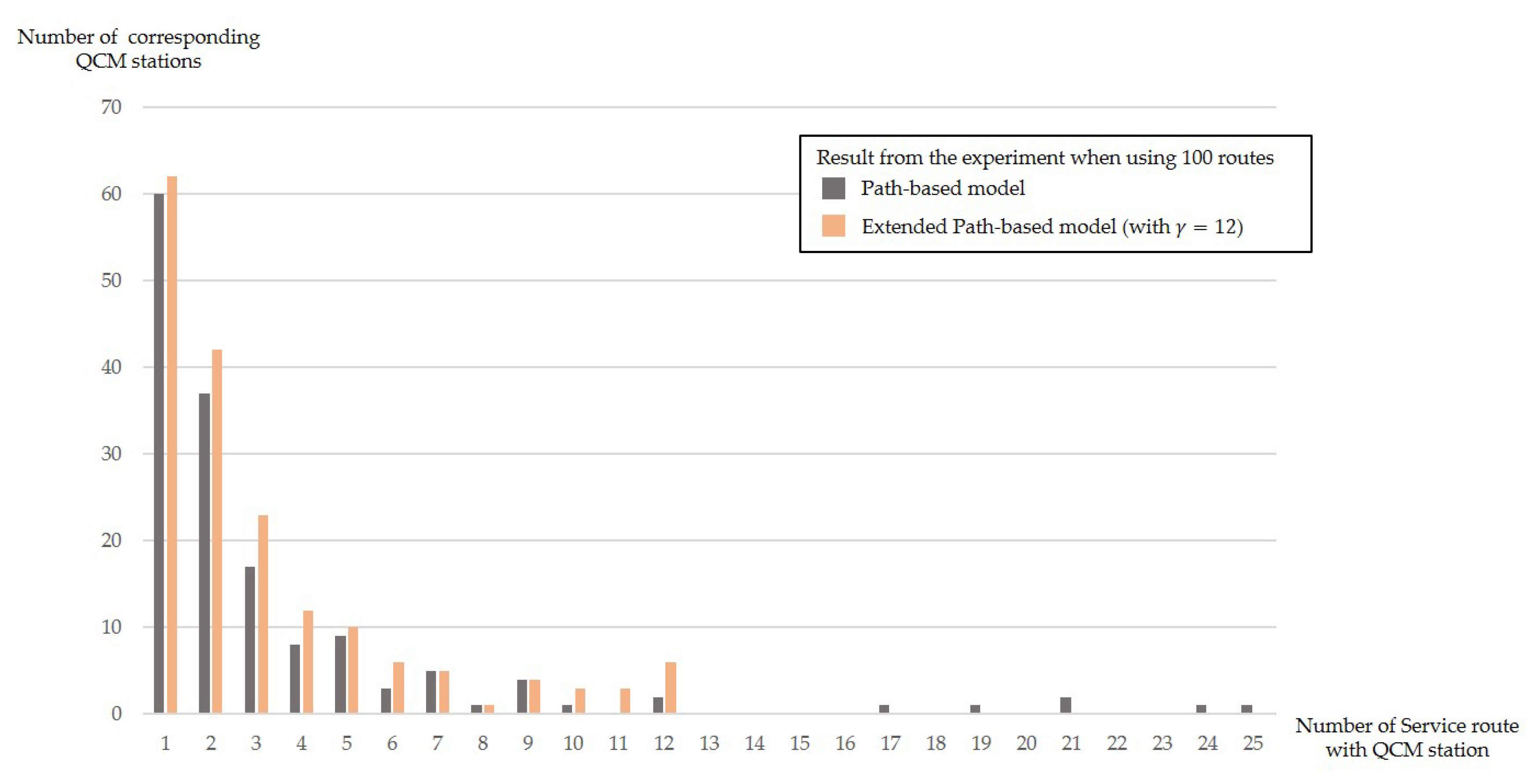
Section 3.5, as a QoS analysis, we introduce additional constraints to the path-based model so that the demand for battery servicing at QCM stations is distributed more evenly over the entire bus transit network and demonstrate that the approach is effective. Most of all, we show the improved flexibility and scalability of the flow-based and path-based models compared to the set-covering model. This paper contributes significantly to the understanding of how to introduce an electric vehicle to an urban area. The varied models can solve this problem and give insight into further studies.
For future work, we can generalize the assumptions used in our problem. First, we assume that all buses depart from the depot at full battery capacity. However, if each bus rotates its route several times, then the initial or final condition of the battery can be different every time. By taking this into account, the improved model can reflect the initial battery level. Moreover, considering the cost of installing each QCM on an individual basis can be meaningful since here we assume the cost of installation is the same for all stations, and, therefore, only focus on minimizing the total number of QCMs. For another problem approach, we can first solve the set-covering model and then solve another scheduling model. The set-covering model only suggests the optimal location of QCM stations but not the specific scheduling, and the result of the flow-based model and path-based model are also restricted by their computational complexity. Thus, proposing additional scheduling problems that utilize the QCM location results of the set-covering model could be another methodological approach, although one that would not guarantee an optimal solution. It is apparent from numerical experiments with real-world data that a heuristic algorithm may be necessary to solve these problems efficiently. Finally, once the strategic decision to install QCMs has been made, operational decisions, such as those concerning battery pack charging/discharging based on usage and the availability of battery packs eligible for battery swapping, need to be addressed.

Author Contributions

Conceptualization, T.C. and S.H.S.; methodology, J.M., Y.J.K., T.C. and S.H.S.; validation, T.C. and S.H.S.; formal analysis, J.M.; investigation, J.M. and Y.J.K.; data curation, J.M. and Y.J.K.; writing—original draft preparation, J.M. and T.C.; writing—review and editing, Y.J.K., T.C. and S.H.S.; supervision, T.C. and S.H.S.; project administration, T.C. and S.H.S.; funding acquisition, T.C. All authors have read and agreed to the published version of the manuscript.

Funding

This research was supported by Basic Science Research Program through the National Research Foundation of Korea (NRF) funded by the Ministry of Education (No. NRF-2018R1D1A1B07047651) and also supported by Korea Institute for Advancement of Technology (KIAT) grant funded by the Korea Government (MOTIE) (P0008691, The Competency Development Program for Industry Specialist).

Acknowledgments

We would like to acknowledge four anonymous reviewers for their constructive and helpful comments.

Conflicts of Interest

The authors declare no conflict of interest.

References

  1. Jeju Introduces Electric Buses with Swapping Battery. Available online: https://kojects.com/2016/07/25/jeju-introduces-electric-buses-with-swapping-battery/ (accessed on 20 November 2019).
  2. China Electric Bus Market—Growth, Trends, and Forecast (2019–2024). Available online: https://www.mordorintelligence.com/industry-reports/china-automotive-electric-bus-market (accessed on 20 November 2019).
  3. Kim, S.; Pelton, R.E.; Smith, T.M.; Lee, J.; Jeon, J.; Suh, K. Environmental Implications of the National Power Roadmap with Policy Directives for Battery Electric Vehicles (BEVs). Sustainability 2019, 11, 6657. [Google Scholar] [CrossRef] [Green Version]
  4. The U.S. Has a Fleet of 300 Electric Buses. China Has 421,000. Available online: https://www.bloomberg.com/news/articles/2019-05-15/in-shift-to-electric-bus-it-s-china-ahead-of-u-s-421-000-to-300 (accessed on 20 November 2019).
  5. Seoul Introduces Electric Bus (Posted on November 15, 2018). Available online: http://koreabizwire.com/seoul-introduces-electric-bus/127453 (accessed on 20 November 2019).
  6. Teoh, L.E.; Khoo, H.L.; Goh, S.Y.; Chong, L.M. Scenario-based electric bus operation: A case study of Putrajaya, Malaysia. Int. J. Transp. Sci. Technol. 2018, 7, 10–25. [Google Scholar] [CrossRef]
  7. Rogge, M.; van der Hurk, E.; Larsen, A.; Sauer, D.U. Electric bus fleet size and mix problem with optimization of charging infrastructure. Appl. Energy 2018, 211, 282–295. [Google Scholar] [CrossRef] [Green Version]
  8. Liu, H.; Wang, D.Z. Locating multiple types of charging facilities for battery electric vehicles. Transp. Res. Part Methodol. 2017, 103, 30–55. [Google Scholar] [CrossRef]
  9. Ko, J.; Shim, J.S. Locating battery exchange stations for electric taxis: A case study of Seoul, South Korea. Int. J. Sustain. Transp. 2016, 10, 139–146. [Google Scholar] [CrossRef]
  10. Chao, Z.; Xiaohong, C. Optimizing battery electric bus transit vehicle scheduling with battery exchanging: Model and case study. Procedia-Soc. Behav. Sci. 2013, 96, 2725–2736. [Google Scholar] [CrossRef] [Green Version]
  11. Kang, Q.; Wang, J.; Zhou, M.; Ammari, A.C. Centralized charging strategy and scheduling algorithm for electric vehicles under a battery swapping scenario. IEEE Trans. Intell. Transp. Syst. 2015, 17, 659–669. [Google Scholar] [CrossRef]
  12. Sarker, M.R.; Pandžić, H.; Ortega-Vazquez, M.A. Optimal operation and services scheduling for an electric vehicle battery swapping station. IEEE Trans. Power Syst. 2014, 30, 901–910. [Google Scholar] [CrossRef]
  13. Pilot Operation of Electric Battery Bus in Pohang, South Korea. Available online: http://www.molit.go.kr/USR/NEWS/m_71/dtl.jsp?lcmspage=3&id=95072972 (accessed on 20 November 2019).
  14. Marinakis, Y. Location routing problemLocation Routing Problem. In Encyclopedia of Optimization; Floudas, C.A., Pardalos, P.M., Eds.; Springer US: Boston, MA, USA, 2009; pp. 1919–1925. [Google Scholar] [CrossRef]
  15. Albareda-Sambola, M. Location-routing. In Location Science; Springer: Berlin/Heidelberg, Germany, 2015; pp. 399–418. [Google Scholar]
  16. Ghiani, G.; Laporte, G. Location-arc routing problems. Opsearch 2001, 38, 151–159. [Google Scholar] [CrossRef]
  17. Corberán, A.; Prins, C. Recent results on arc routing problems: An annotated bibliography. Networks 2010, 56, 50–69. [Google Scholar] [CrossRef]
  18. Prodhon, C.; Prins, C. A survey of recent research on location-routing problems. Eur. J. Oper. Res. 2014, 238, 1–17. [Google Scholar] [CrossRef]
  19. Golumbic, M.C.; Hartman, I.B.A. Graph Theory, Combinatorics and Algorithms: Interdisciplinary Applications; Springer Science & Business Media: Berlin/Heidelberg, Germany, 2006; Volume 34. [Google Scholar]
  20. Amaya, A.; Langevin, A.; TréPanier, M. The capacitated arc routing problem with refill points. Oper. Res. Lett. 2007, 35, 45–53. [Google Scholar] [CrossRef]
  21. Xing, L.; Rohlfshagen, P.; Chen, Y.; Yao, X. An evolutionary approach to the multidepot capacitated arc routing problem. IEEE Trans. Evol. Comput. 2009, 14, 356–374. [Google Scholar] [CrossRef] [Green Version]
  22. Bektaş, T.; Elmastaş, S. Solving school bus routing problems through integer programming. J. Oper. Res. Soc. 2007, 58, 1599–1604. [Google Scholar] [CrossRef]
  23. Yang, J.; Sun, H. Battery swap station location-routing problem with capacitated electric vehicles. Comput. Oper. Res. 2015, 55, 217–232. [Google Scholar] [CrossRef]
  24. Boccia, M.; Sforza, A.; Sterle, C. Flow intercepting facility location: Problems, models and heuristics. J. Math. Model. Algorithms 2009, 8, 35–79. [Google Scholar] [CrossRef]
  25. Desaulniers, G.; Desrosiers, J.; Solomon, M.M. Column Generation; Springer Science & Business Media: Berlin/Heidelberg, Germany, 2006; Volume 5. [Google Scholar]
  26. Seoul Open Data Center. Available online: https://data.seoul.go.kr/ (accessed on 20 November 2019).
Figure 1. Operational concept of a bus station with Quick Charger Machine (QCM) [13].
Sustainability 12 01142 g001
Figure 2. Basic idea of set-covering formulation.
Sustainability 12 01142 g002
Figure 3. Public bus transit network with stations in the Seoul metropolitan area, South Korea.
Sustainability 12 01142 g003
Figure 4. Graphical summary of the experimental results of the set-covering model.
Sustainability 12 01142 g004
Figure 5. Plots of the optimal QCM installations obtained from the set-covering model.
Sustainability 12 01142 g005
Figure 6. Graphical summary of the experimental results of the flow-based model.
Sustainability 12 01142 g006
Figure 7. Plots of the optimal QCM installations obtained from the flow-based model.
Sustainability 12 01142 g007
Figure 8. Graphical summary of the experimental results of the path-based model.
Sustainability 12 01142 g008
Figure 9. Plots of the optimal QCM installations obtained from the path-based model.
Sustainability 12 01142 g009
Figure 10. Comparison of model computational times.
Sustainability 12 01142 g010
Figure 11. The number of bus routes each QCM station serves.
Sustainability 12 01142 g011
Figure 12. The detailed QoS result for 100 routes.
Sustainability 12 01142 g012
Table 1. Mathematical notations used in this paper.
Sets and Parameters
N = 1 , 2 , , N . Set of bus stops
A = ( i , j ) | i , j N , j ( i ) is directly accessible from i ( i . e . , i j ) . Set of arcs
N s N Set of potential bus stops equipped with battery swapping facility (Quick Change Machine (QCM))
R = 1 , 2 , , R . Set of bus routes
D o N s Set of origins (depots) for all bus routes
D d N s Set of destinations (depots) for all bus routes
r Total number of bus stops on route r R
D m a x Maximum travel distance per charge
T r ( n 1 r , n 2 r , , n r r ) . Ordered sequence of bus stops on route r R where n i r N for all i = 1 , 2 , , r . Note that (i) ( n i r , n i + 1 r ) A for i = 1 , , r - 1 and (ii) n i r r n j r holds for any i and j such that i < j where the precedence relationship in the ordered sequence is denoted by r .
T r = n 1 r , n 2 r , , n r r . Ordered set of bus stops on route r R
D r ( α , β ) Travel distance from bus stop α N to bus stop β N on route r R
N s r = T r N s . Set of potential QCMs in T r
T α r = α n i r , n i + 1 r , , n j r T r . Maximal ordered subset (MOS) of T r , starting from a potential QCM α N s r such that D r ( n i r , n j r ) D m a x and D r ( n i r , n j + 1 r ) > D m a x
  • For given T α r = α n i r , n i + 1 r , , n j r β , D r ( α , β ) is the maximal distance that e-Bus can drive without any battery swapping, assuming that a battery swap is performed at α N s .
Decision variables
y i 1 if a QCM is located at bus stop i N s , and 0 otherwise
Table 2. Additional notations for flow-based formulation.
Sets and Parameters
L r ( n i r ) Last bus stop where a QCM is installed in T n i r r (i.e., L r ( n i r ) = n j r if the ordered set of T n i r r N s with respect to r is equal to n i r , , n j r ).
I r ( α ) T κ r { α } N s r where L r ( κ ) = α . Note that I r ( α ) = ϕ if α D o .
O r ( α ) T α r { α } N s r . Note that O r ( α ) = ϕ if α D d .
Decision variables
x α κ r 1 if a bus on the route r performs a battery swapping at QCM α and the next immediate battery swapping is performed at QCM κ where α , κ N s r and α r κ , and 0 otherwise.
Table 3. Additional notations for path-based formulation.
Sets and Parameters
P ( r ) Set of paths for the route r R where a path is a set of consecutive sub-routes where connecting points correspond to QCMs
N r ( l ) Set of stations which the path l for the route r visits.
Decision variables
x l r 1 if the path l P ( r ) is selected, and 0 otherwise.
Table 4. Experimental results of the set-covering model.
# of Routes
(# of Stations)
Optimal # of QCM StationsAvg. CPU Time (sec)Max Gap between CPU Times (sec)# of Variables# of Constraints
5 (441)120.0860.012441595
10 (822)200.3010.0768221185
20 (1611)370.7080.07116112422
30 (2286)530.9680.06622863631
40 (2681)651.3260.41126814710
50 (3058)732.0010.44430585822
60 (3597)822.4930.55835977074
70 (3929)1022.5610.32939297880
80 (4235)1212.8480.18642358537
90 (4435)1373.0340.1144359282
100 (4732)1523.3780.121473210,287
200 (7008)2565.6140.233700818,194
300 (8059)3157.7251.17805925,352
400 (8937)3829.2460.377893731,492
500 (10,934)5499.870.410,93434,908
600 (12,650)7219.7930.45912,65037,799
635 (13,191)78210.3131.35713,19138,636
Table 5. Experimental results of the flow-based model.
# of Routes
(# of Stations)
Optimal # of QCM StationsAvg. CPU Time (sec)Max Gap between CPU Times (sec)# of Variables# of Constraints
5 (441)1216.8350.202972,846240,434
10 (822)2135.8911.2232,205,658681,564
15 (1230)28122.6671.6586,757,6621,816,809
18 (1552)32687.1255.80510,757,6624,816,809
20 (1611)372356.15615.42534,541,55112,426,973
30 (2286)-----
40 (2681)-----
50 (3058)-----
Table 6. Experimental results of the path-based model.
# of Routes
(# of Stations)
Optimal # of QCM StationsAvg. CPU Time (sec)Max Gap between CPU Times (sec)# of Variables# of ConstraintsAvg. # of Iterations
5 (441)1215.7810.04251520286
10 (822)2160.4180.084956422215
15 (1230)28285.1181.5841355569348
20 (1611)371296.6213.5841950744586
30 (2286)532874.5166.8713125968863
40 (2681)654225.88910.668485712681153
50 (3058)735826.14615.13922,61816051868
60 (3597)827361.41123.58430,52028412735
70 (3929)1028165.15643.45837,21138693868
80 (4235)12110,041.453167.16543,58454125066
90 (4435)13714,025.584304.54551,25181696166
100 (4732)15223,218.975518.10758,51898877259
200 (7008)25681,540.145682.618135,68534,81525,015
300 (8059)315345,154.587822.123209,87165,03668,121
Table 7. Comparison of the computational results of the three models.
Set-Covering ModelFlow-Based ModelPath-Based Model
# of Routes
(# of Stations)
CPU Time (sec)Optimal # of QCM StationsCPU Time (sec)Optimal # of QCM StationsCPU Time (sec)Optimal # of QCM Stations
5 (441)0.0861216.8351215.78112
10 (822)0.3012135.8912160.41821
15 (1230)0.51428122.66728285.11828
20 (1611)0.708372356.156371296.62137
30 (2286)0.96853--2874.51653
40 (2681)1.32665--4225.88965
50 (3058)2.00173--5826.14673
60 (3597)2.49382--7361.41182
70 (3929)2.561102--8165.156102
80 (4235)2.848121--10,041.453121
90 (4435)3.034137--14,025.584137
100 (4732)3.378152--23,218.975152
200 (7008)5.614256--81,540.145256
300 (8059)7.725315--345,154.587315
400 (8937)9.246382----
500 (10,934)9.87549----
600 (12,650)9.793721----
635 (13,191)10.313782----
Table 8. Additional notation for the extended path-based formulation.
Additional Parameter
γ Maximally allowable number of bus routes stopping at a QCM station for battery swapping
Table 9. Computational result with(out) Quality of Service (QoS) constraints in the path-based model.
Original Path-Covering ModelExtended Path-Based Model
# of Routes
(# of Stations)
# of QCM StationsMaximum Flock ( γ )Variance of FlockingCPU Time (sec)# of QCM StationsMaximum Flock ( γ )Variance of FlockingCPU Time (sec)
5 (441)1241.40115.7811420.86316.115
10 (822)2171.98760.4182241.47869.054
15 (1230)2892.081285.1182951.975308.487
20 (1611)3791.9931296.6213951.0721583.142
30 (2286)5391.9742874.5165551.8823593.145
40 (2681)6592.0134225.8896751.3425451.396
50 (3058)7391.9555826.1467651.2779828.708
60 (3597)82112.1547361.4118571.27010,453.203
70 (3929)102153.3778165.15610481.48313,717.462
80 (4235)121213.67010,041.453125102.49512,903.267
90 (4435)137243.82314,025.584141102.47819,032.717
100 (4732)152254.28423,218.975158122.87634,317.645
Table 10. Computational result as the γ value changes.
Extended Path-Based Model Experimented with 60 Routes
γ # of QCM StationsMaximum FlockVariance of FlockingCPU Time (sec)
6infeasible---
78571.27010,453.204
88481.6219358.721
98491.8198715.780
1082102.0847521.184
11 (no restict)82112.1547361.411

