Impact of Strategic Cooperation under Competition on Green Product Manufacturing

Abstract

This study explores the optimal pricing and investment decision for two competing green supply chains, both consisting of a manufacturer and an exclusive retailer. Our focus is to explore, does the strategic integration decision with rivals at the horizontal level or with partners at the vertical level have any effect on green product types? The results reveal the following insights: retailer-retailer strategic integration at downstream level leads to a sub-optimal total supply chain profit and green quality level for a development-intensive green product. Two competing manufacturers can produce products at a higher level if they are vertically integrated with respective retailers. Manufacturer-manufacturer integration at upstream level sometimes leads to higher profits and product quality level if cross price-elasticity of consumers is high. However, an opposite phenomenon is observed while they are selling for a marginal-intensive green product, horizontal integration can improve green quality levels, but supply chain members will receive a lower profit. Therefore, selection of green product types and strategic integration decision are interrelated to achieve the profit maximization goal along with the aim to offer products at a higher green quality level. Vertical integration strategy can outperform horizontal integration strategy, especially if cross-price elastic for green products remain high.

1. Introduction

Over the last couple of decades, investment decisions of firms in green quality improvement have been viewed as one of the important solutions to accomplish both environmental protection and economic growth [1]. Firms are involved in green business for many reasons, such as social responsibility, stakeholder and government pressure, competitiveness, consumers’ pressure, etc. [2,3]. A recent survey by Accenture reported that 83% of consumers increasingly favor products that embrace purpose and sustainability [4]. To elicit pro-environmental aspects of influencing consumption, an increasing number of manufacturers make green technology investments. However, the cost of investment in green technology is usually substantial, and found to be one of the key obstructions in green product manufacturing [5,6,7,8]. Investment decisions further become problematic in the presence of competitors selling similar types of product, as demands for substitute products are negatively correlated. In this study, we analyze the equilibrium of two competing green supply chains (GSCs), both of which consist of a single manufacturer, selling its substitute products exclusively through a single retailer. The proposed GSC structures fit industries such as a premium gasoline, soft drinks, garments, foot wears, electric vehicles, electronics accessories, etc., where a manufacturer trades with an exclusive retailer. In this study, we focus on the investment decisions of two types of green products under five strategic decision structures.

As a strategic measure, integration with a horizontal competitor [9] or ‘collusion formation’ [10] is not unusual in the business environment. For example, stable collaborative relationships between Apple and Samsung [11] support this possibility. Competing members are interested in strategic integration in anticipating the achievement of business goals such as increasing the current joint market size, developing products with new features to protect the present and future share of the market, and to conquer a larger share of the market that remains [12]. Although the literature on horizontal integration is scanty regarding green supply management, but advantages and disadvantages of vertical integration are well documented [9,13]. Therefore, it is necessary to conduct a systematic analysis for evaluating interrelationships among strategic integration, green product type, and investment for manufacturers, which can help managers to identify the pros and cons that affect GSCs performance. However, there has been little analytical research in this direction so far that explicitly provides a comparative overview under supply chain competition.

This study aims to address the gap by studying this effect of green investment decisions to produce development-intensive green products (DIGPs) and marginal-intensive green products (MIGPs). Investment decisions to improve quality have received considerable attention in the existing literature [14,15,16]. As reported by Dey et al. [17], Zhou and He [18], green products can be classified into three categories: MIGPs, DIGPs, and MDIGPs (marginal and development-intensive green products). For DIGPs, the total investment in green technology depends on the green quality level [18], whereas for MIGPs investment in green technology directly varies with the production quantity [17]. Please note that MDIGPs are both development and marginal-cost-intensive [19]. However, to the best our knowledge, a comparative analysis of investment decisions on green product types under competition has not been yet conducted. From the above discussion, we realize the following issues are worthy of investigation:

• When competing manufacturers make investment decisions in improving green quality levels, will the nature of the green product types play a decisive role? If so, how does the manufacturer’s product type selection affect the performance of GSCs and consumers?
• How does the strategic integration decision under two competing GSCs affect the green quality level? Does the integration with a horizontal competitor or integration with vertical member favor green supply chain practice? Does that effect remain indistinguishable irrespective of product type?

To answer the above questions, we study optimal decisions in a two-manufacturer-two-retailer supply chain setting. First, we analyze the scenario where all the members optimize their respective profits and consider the result as a benchmark for further analysis. Next, we explore optimal decisions in two game structures to explore the effect of horizontal integration. In the first game structure, two upstream manufacturers jointly decide wholesale prices and green quality levels of product that maximize total upstream profits [10], and, in the second game structures, two retailers jointly decide retail prices by maximizing the sum of downstream profits [9]. Finally, we consider two game structures to explore the effect of vertical integration. Consequently, we explore optimal decisions where both GSCs are vertically integrated and members of one GSC are vertically integrated while members in other GSC strict to imply decentralized decision. Therefore, we formulate models under ten different scenarios to draw on investment decisions in improving the green quality level for DIGPs and MIGPs. We compare optimal decisions, discuss managerial implications, and provide insights to make strategic integration decisions associated with green product design and selling. This paper contributes to the literature in the following ways. First, we determine and compare optimal decisions under five decision structures to obtain a comprehensive overview of investment decisions under competition. This will help the decision-makers to identify whether they should look for strategic integration with their rivals or partners. Second, we explore optimal outcomes for both MIGPs and DIGPs, and highlight the pros and cons of each strategic decision. Finally, the study will help in understanding how consumers are affected under such strategic deals and whether the regulatory agencies need to intervene if competing members are interested in fulfilling only a profit maximization goal.

Literature Review

Over the past three decades, the optimal decisions in a two-manufacturer-two-retailer SCs competition have been studied by several researchers. However, more recently, this stream of research has gained increasing attention [9,20,21,22,23]. We summarized some of the key studies focused on the optimal decision under competition in the following

Table 1. Studies on two-manufacturer-two retailer supply chains.

Study	Game Structure	Distribution	Demand Function	Information
Ha and Tong (2008) [22]	DD, II		Inverse Price-dependent	Symmetric & asymmetric
Anderson and Bao (2010) [24]	DD, II	Direct	Price-dependent	Symmetric
Li et al. (2013) [25]	DD	Direct, Cross	Price, and service level	Symmetric
Zhou and Cao (2014) [13]	DD, II, ID	Direct	Price, and service level	Symmetric
Fang and Shoub (2015) [26]	DD, II, ID	Direct	Price-dependent	Symmetric
Xei (2015) [27]	DD, II	Direct	Price and energy saving levelwithout cross elasticity	Symmetric
Bian et al.(2016) [28]	DD	Direct	Price-dependent	Symmetric & asymmetric
Li and Li (2016) [29]	DD, II, ID	Direct	Service level	Symmetric
Wang et al. (2016) [30]	DD	Direct	Price-dependentisoelastic demand	Symmetric
Hafezalkotob (2017) [31]	DD, II, CC	Direct	Price and energy saving level	Symmetric
Hafezalkotob (2018) [32]	DD, II	Direct	Price and energy saving level	Symmetric
Wei et al. (2019) [9]	DD, II, CCMC, RC	Direct	Price-dependent	Symmetric
Bian et al. (2020) [10]	DD, MC, RC, TS	Direct, Cross	Inverse Price-dependent	Symmetric
Present Study	MC, RC, II, DD, ID	Direct	Price, and green quality level	Symmetric

$DD$—two decentralized SCs, $ID$—one integrated and one decentralized SCs, $II$—two integrated SCs, $CC$—all members are integrated, $MC$—two upstream manufacturers are integrated, $RC$—two downstream retailers are integrated, $TS$—grim trigger strategy.

.

From Table 1, it is clear that a group of researchers studied the influence of information asymmetry on the performance of SC members [22,33]. However, the authors explored the effect of only a limited number of game scenarios. Taking another perspective, some researchers [10] compare the performance of supply chain members under competition by allowing cross-selling activities, i.e., instead of selling their products through an exclusive retailer, they sell products with both retailers. However, they ignore the effect of non-pricing factors influencing market demand. This study is lie with previous studies conducted by Zhou and Cao [13], Wei et al. [9] where the authors analyzed decisions under different game settings. From Table 1, we observe that there is a limited number of studies that take account of the non-pricing factors in the demand function. In contrast to the existing literature, we consider the influence of product types under competition. The present work is similar to Zhou and He [18], where the authors consider both DIGPs and MIGPs, but the authors analyzed optimal decisions under different supply chain structures, namely single-manufacturer-single-retailer, single-manufacturer-two-retailer, and two-retailer-two-manufacturer where members are maximized their individual profits. However, we explore decisions under competition in various game structures to find answer to: how does integration among members at the horizontal or vertical level affect the performance of GSCs?

This study contributes to the sustainable supply chain management research stream by analyzing green product manufacturing decisions. We refer some recent work by [2,34,35,36] for various aspects in this research direction. Due to a growing awareness among consumers about the environmental impact on products they procure, it is always an important issue to study the transition of supply chain decisions by considering the impact of green quality sensitivity in-demand function. Therefore, researchers studied characteristics of supply chain equilibrium where the demand function is influenced by the green quality level and retail price [37,38,39,40,41,42,43,44]. This group of researchers primarily focused on the equilibrium decisions under the various game-theoretic models or discuss performance under various supply chain coordination mechanisms, generally under a single manufacturer-single retailer setting. In addition, most of the studies consider the green technology investment for DIGPs, and only a limited number of studies, mostly in the last couple of years, explored supply chain decisions for MIGPs. In addition to the work by Zhou and He [18], recently, a handful of research highlighted the impact of MIGPs and DIGPs, such as Dey et al. [17] studied the impact of strategic inventory on the product manufacturing decision, Li et al. [15] discussed the effect of the retailer’s fairness concern. Therefore, the affect of green product types is also not fully explored in the existing literature under competition.

Therefore, this study contributes to the research stream, mainly supply chain competition and green product design and pricing, aiming to help GSC participants to make decisions regarding strategic integration horizontally and vertically to maximize their respective profit and produce products at a higher green quality level. Therefore, this research could aid environmental monitoring agencies in making environmental regulation policies regarding strategic alliance under competition.

2. Problem Description

Two competing GSCs are considered (i = 1, 2), each consists of a manufacturer ($M_i$) and an exclusive retailer ($R_i$). It is considered that $M_1$ sells the substitutable products through $R_1$ and $M_2$ sells the product through $R_2$, respectively, i.e., cross-selling is not allowed [9,28]. We investigate the optimal decisions under five-game structures. Under game structure $DD$, each member in competing GSCs implement a decentralized decision, which is similar to [10,13]. Under game structure $MC$, two upstream manufacturers are integrated by centralized management and set wholesale prices and green quality levels that maximize the sum of profits for two manufacturers [9]. Under game structure $RC$, two downstream retailers are integrated by a centralized management, and set retail prices that maximize the sum of profits for two retailers [9]. Therefore, game structures $MC$ and $RC$ represent the characteristics of GSCs when members are integrated horizontally. To explore the effect of vertical integration, we derive optimal decisions in two-game structures. Under game structure $ID$, participants of one of the GSC are integrated by a centralized management; however, members in other GSC remain decentralized [13]. Finally, under game structure $II$, members in each GSC are integrated by centralized managers and implement coordinated decisions [13]. To formalize analytical models, the following assumptions are made:

Assumption 1.

The demand function ($D_i^z$), for the $ith$ product is linear function of retail prices ($p_i^z$), and the green quality level (${\theta }_i^z$), and the functional form is presented below:

$$D_i^z=a-p_i^z+\beta p_j^z+\gamma {\theta }_i^z-\delta {\theta }_j^z,i=1,2,j=3-i$$

(1)

Demand for each product is proportional with the green quality level sensitivity ($\gamma$) of that product and price sensitivity ($\beta$) of the other product, and inversely proportional with own price and green quality level sensitivity ($\delta$) of the other product [32,45]. In above demand function, if $\beta =\delta =0$, it is similar to [46]. If $\gamma =\delta =0$ the demand function becomes price dependent which is similar to [9,10]. It is assumed that the self-price elasticity coefficient is more important than that of competitor ($\beta <1$) and green quality level sensitivity is more important than that of competitor($\gamma >\delta$).

Assumption 2.

Two types of green product, i.e., DIGPs and MIGPs, are considered. Both manufacturers are investing to improve the green quality level to remain competitive. For DIGPs, both manufacturers invest to improve green quality level, which is independent of sales volume and investment cost is considered to be a quadratic function of the green quality level, i.e., total investment for each manufacturer is ${\eta }_1{{\theta }_i^{z_1}}^2$ [39,42]. For MIGPs, both manufacturers invest on per-unit product and it is dependent on sales volume, i.e., investment for each manufacturer is $D_i^{z_2}{\eta }_2{{\theta }_i^{z_2}}^2$ [17,18]. To enable a fair comparison among the optimal decisions for different scenarios and for analytical simplicity, we assume investment efficiencies for both manufacturers are equal [47,48]. DIGPs require significant investment before large-scale production (e.g., new-energy automobiles or new technologies). Conversely, MIGPs needs installation of new components or to use different material types to achieve environmental friendliness [49].

Assumption 3.

There will always have a symmetric information about cost, the green quality level and demand parameters between two GSC members [48,50]. For the reminder of the study, we assume that ${\eta }_1>max\left\{\frac{{(2\gamma -\beta \delta )}^2}{4(4-{\beta }^2)(2-{\beta }^2)},\frac{{\gamma }^2}{4},\frac{{(\gamma -\delta )}^2}{4(2-3\beta +{\beta }^2)},\frac{{(\gamma +\delta )}^2}{4(2+3\beta +{\beta }^2)},\frac{(2+{\beta }^2)({\gamma }^2+{\delta }^2)-6\beta \gamma \delta }{4(4-5{\beta }^2+{\beta }^4)}\right\}$ and ${\eta }_2>max\left\{\frac{2(2-15\beta +6{\beta }^2-{\beta }^3)\gamma \delta -(2+\beta -18{\beta }^2+7{\beta }^3){\gamma }^2+(14-9\beta +2{\beta }^2+{\beta }^3){\delta }^2}{4a(1-\beta )(1+\beta )(2+\beta )},\frac{4(2-\beta )-3(3-\beta ){\gamma }^2+2\gamma \delta }{4a}\right\}$, respectively. Two conditions not only ensure that there must be a threshold for the investment efficiency limits of each manufacturer’s green technology investment, but conditions are sufficient for many subsequent analytical results related to the existence of optimal decision in ten scenarios. In addition, wholesale prices, green quality levels, retail prices, and individual and total GSC profits remain positive under these conditions.

The following notations in

Table 2. Notations.

Notations	Descriptions
Indices
i	index for ith GSC, $i\in \{1,2\}$
x	index for game structures, $x\in \{DD,MC,RC,II,ID\}$
y	index for product types, $y\in \{D,M\}$
z	index for decision scenarios, $z=z_1\cup z_2$, where $z_1\in \{DDD,MCD,RCD,IDD,IID\}$ representsscenarios for DIGPs and $z_2\in \{DDM,MCM,RCM,IDM,IIM\}$ represents scenarios for MIGPs
Parameters
a	market potential of each GSC ($a>0$)
$\beta$	the cross-price sensitivity of consumers between two products, $\beta \in [0,1)$
$\gamma$	green quality level sensitivity of consumers of own GSC, $\gamma \in (0,1)$
$\delta$	green quality level sensitivity of consumers with that of rival GSC, $\delta \in [0;1)$ ($\delta <\gamma$)
${\eta }_1$	coefficient investment efficiency for two manufacturers for DIGPs, ${\eta }_1>0$
${\eta }_2$	coefficient investment efficiency for two manufacturers for MIGPs, ${\eta }_2>0$
Variables
$w_i^z$	wholesale price of per unit product for ith GSC
$p_i^z$	retail price of per unit product for ith GSC
${\theta }_i^z$	the green quality level of ith product
${\pi }_{ri}^z$	profit of the ith retailer
${\pi }_{mi}^z$	profit of the ith manufacturer
${\pi }_{ci}^z$	total profit of the ith GSC
$Q_i^z$	sales volume of ith GSC

are used to distinguish optimal decisions. Please note that we use additional symbols to simplify mathematical expressions, and those are presented in Appendix J.

Based on the above assumption and notation, profit functions for two retailers and manufacturers (i = 1, 2) for the DIGPs are formed as follows:

$$\left\{\begin{array}{cc}\hfill & {\pi }_{ri}^{z_1}\left(p_i^{z_1}\right)=(p_i^{z_1}-w_i^{z_1})D_i^{z_1}\hfill \\ \hfill & {\pi }_{mi}^{z_1}(w_i^{z_1},{\theta }_i^{z_1})=w_i^{z_1}{D}_i^{z_1}-{\eta }_1{{\theta }_i^{z_1}}^2(i=1,2)\hfill \end{array}\right.$$

(2)

Similarly, profit functions for two retailers and manufacturers for MIGPs are as follows:

$$\left\{\begin{array}{cc}\hfill & {\pi }_{ri}^{z_2}\left(p_i^{z_2}\right)=(p_i^{z_2}-w_i^{z_2})D_i^{z_2}\hfill \\ \hfill & {\pi }_{mi}^{z_2}(w_i^{z_2},{\theta }_i^{z_2})=(w_i^{z_2}-{\eta }_2{{\theta }_i^{z_2}}^2)D_i^{z_2},(i=1,2)\hfill \end{array}\right.$$

(3)

In the following section, we explore optimal decisions in various scenarios.

3. Model Solutions and Discussions

In this section, we introduce ten models to explore the effects of horizontal and vertical integration on green product design. First, we consider the completely decentralized model and use its equilibrium outcome as a benchmark in subsequent analysis. Second, we formulate the models where members are horizontally integrated, and explore the condition and how it affects product green quality level. Finally, we establish models associated with vertically integrated scenarios and compare results.

3.1. Optimal Decisions in Scenarios DDD and DDM

In a decentralized decision, each member in two competing GSCs optimizes their respective profits. We assume that two upstream manufacturers have more dominant roles, i.e., upstream manufacturers act as the Stackelberg game leaders, while downstream retailers are the Stackelberg game followers. The decision under this scenario is commonly discussed in the literature on supply chain competition as noted in Table 1. We use backward induction to find complete equilibrium solution, the sequence of events in Scenarios DDD and DDM are as follows:

Step 1: Both manufacturers decide their respective wholesale prices ($w_i^z,z=ddd,ddm$) and green quality levels (${\theta }_i^z$) to maximize their individual profits.

Step 2: Two retailers decide their respective retail prices ($p_i^z$) to maximize their own profits.

Therefore, we have the following optimization problems:

$$\left\{\begin{array}{cc}\hfill & \underset{(w_1^z,{\theta }_1^z)}{max}{\pi }_{m1}^z+\underset{(w_2^z,{\theta }_2^z)}{max}{\pi }_{m2}^z\hfill \\ \hfill & \left\{\begin{array}{cc}\hfill & \underset{p_1^z}{max}{\pi }_{r1}^z+\underset{p_2^z}{max}{\pi }_{r2}^z.\hfill \end{array}\right.\hfill \end{array}\right.$$

(4)

Optimal decisions in Scenarios DDD and DDM are presented in Propositions 1 and 2, respectively. We refer to Appendix A for the detailed derivation of the optimal decision in Scenario DDD. The derivation of the optimal decision in Scenario DDM is similar to Scenario DDD, hence we omitted the detail.

Proposition 1.

Optimal decision in Scenario DDD is as follows:

$w_i^{ddd}=\frac{2a(4-{\beta }^2){\eta }_1}{{\Delta }^{ddd}}$; $p_i^{ddd}=\frac{4a(3-{\beta }^2){\eta }_1}{{\Delta }^{ddd}}$; ${\theta }_i^{ddd}=\frac{a(2\gamma -\beta \delta )}{{\Delta }^{ddd}}$; ${\pi }_{ri}^{ddd}=\frac{4a^2{\eta }_1^2{(2-{\beta }^2)}^2}{{{\Delta }^{ddd}}^2}$; ${\pi }_{mi}^{ddd}=\frac{a^2{\eta }_1(4(8-6{\beta }^2+{\beta }^4){\eta }_1-{(2\gamma -\beta \delta )}^2)}{{{\Delta }^{ddd}}^2}$; ${\pi }_{ci}^{ddd}=\frac{a^2{\eta }_1(8(6-5{\beta }^2+{\beta }^4){\eta }_1-{(2\gamma -\beta \delta )}^2)}{{{\Delta }^{ddd}}^2}$; $Q_i^{ddd}=\frac{2a(2-{\beta }^2){\eta }_1}{{\Delta }^{ddd}}$.

Proposition 2.

Optimal decision in Scenario DDM is as follows:

$w_i^{ddm}=\frac{4a(2-{\beta }^2)(2+\beta ){\eta }_2+4(3+\beta )\gamma +(4+3\beta )\beta {\delta }^2-2(4+6\beta +{\beta }^2)\gamma \delta }{4(2-{\beta }^2)(4-\beta -2{\beta }^2){\eta }_2}$;

$p_i^{ddm}=\frac{8a(6-5{\beta }^2+{\beta }^4){\eta }_2+4(7-2{\beta }^2){\gamma }^2+4(6+4\beta -2{\beta }^2-{\beta }^3)\gamma \delta +\beta (12+\beta -4{\beta }^2){\delta }^2}{4(2-\beta )(2-{\beta }^2)(4-\beta -2{\beta }^2){\eta }_2}$; ${\theta }_i^{ddm}=\frac{2\gamma -\beta \delta }{2(2-{\beta }^2){\eta }_2}$;

${\pi }_{ri}^{ddm}=\frac{{(4a{(2-{\beta }^2)}^2{\eta }_2+4(1+\beta -{\beta }^2){\gamma }^2-2(4-{\beta }^3)\gamma \delta +\beta (4-\beta +{\beta }^2){\delta }^2)}^2}{16{(2-\beta )}^2{(2-{\beta }^2)}^3{(4-\beta +2{\beta }^2)}^2{\eta }_2^2}$;

${\pi }_{mi}^{ddm}=\frac{(2+\beta ){(4a{(2-{\beta }^2)}^2{\eta }_2+4(1+\beta -{\beta }^2){\gamma }^2-2(4-{\beta }^3)\gamma \delta +\beta (4-\beta +{\beta }^2){\delta }^2)}^2}{16(2-\beta ){(2-{\beta }^2)}^3{(4-\beta +2{\beta }^2)}^2{\eta }_2^2}$;

${\pi }_{ci}^{ddm}=\frac{(3-{\beta }^2){(4a(2+\beta )(2-{\beta }^2){\eta }_2+4(3+\beta ){\gamma }^2-2(4+6\beta +{\beta }^2)\gamma \delta +\beta (4+3\beta ){\delta }^2)}^2}{8{(2-\beta )}^2{(2-{\beta }^2)}^3{(4-\beta +2{\beta }^2)}^2{\eta }_2^2}$;

$Q_i^{ddm}=\frac{4a{(2-{\beta }^2)}^2{\eta }_2+4(1+\beta -{\beta }^2){\gamma }^2-2(4-{\beta }^3)\gamma \delta +\beta (4-\beta +{\beta }^2){\delta }^2}{4(2-\beta )(2-{\beta }^2)(4-\beta +2{\beta }^2){\eta }_2}$

From Propositions 1 and 2, we made the following remarks:

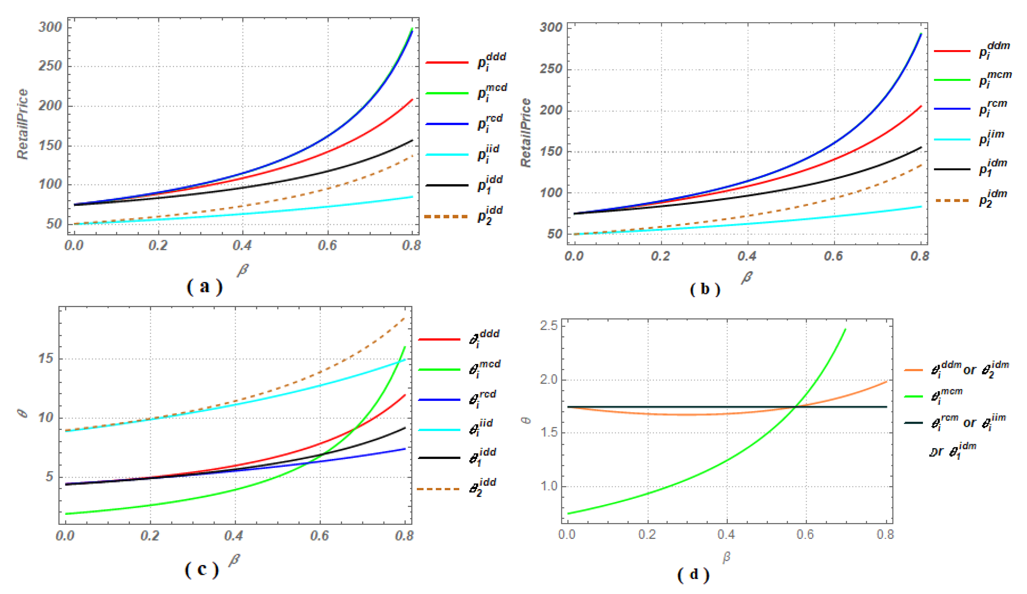
• The product green quality is directly affected by increasing market potential for DIGPs, but not MIGPs.
• The product green quality levels of DIGPs and MIGPs increase with $\beta$ and $\gamma$, and decrease with $\delta$ and ${\eta }_i$.

We refer to Appendix H for all relations exploring the nature of green quality levels in subsequent scenarios with respect to parameters. The increasing consumers sensitivity with green quality level motivates both manufacturers to improve quality levels; however, if the manufacturers need to invest more to improve product green quality levels, then market prices will be high, consequently demand decreases and product green quality level decreases. The result reflects this fact. The ratios of the profits between retailers and manufacturers for DIGPs and MIGPs are $\frac{{\pi }_{ri}^{ddd}}{{\pi }_{mi}^{ddd}}=\frac{4{(2-{\beta }^2)}^2{\eta }_1}{4(2-{\beta }^2)(4-{\beta }^2){\eta }_1-{(2\gamma -\beta \delta )}^2}$ and $\frac{{\pi }_{ri}^{ddm}}{{\pi }_{mi}^{ddm}}=\frac{2-{\beta }^2}{4-{\beta }^2}$, respectively. Therefore, green quality level sensitivity or investment efficiency do not affect the profit share between GSC members for MIGPs, only cross-price elasticity appears as a decisive parameter.

3.2. Influence of Horizontal Integration

In this subsection, we discuss the effect of horizontal integration at each echelon on product green quality level and profits for each members.

3.2.1. Optimal Decisions in Scenarios MCD and MCM

In Scenarios MCD and MCM, two upstream manufacturers are integrated by a horizontal manager. Wholesale prices and green quality levels are determined by maximizing the sum of profits of two upstream manufacturers. According to [10], the decision structure represents upstream collusion. The sequence of decisions is presented below:

Step 1: First, upstream manager sets wholesale prices ($w_i^z$) and green quality levels (${\theta }_i^z$) by maximizing sum of profits of two upstream manufacturers, i.e., ${\pi }_m^z={\pi }_{m1}^z+{\pi }_{m2}^z$, $z=mcd,mcm$.

Step 2: Then two downstream retailers decide their respective retail prices ($p_i^z$) by maximizing their respected profits.

Therefore, we have the following optimization problems:

$$\left\{\begin{array}{cc}\hfill & \underset{(w_1^z,w_2^z,{\theta }_1^z,{\theta }_2^z)}{max}{\pi }_m^z={\pi }_{m1}^z+{\pi }_{m2}^z\hfill \\ \hfill & \left\{\begin{array}{cc}\hfill & \underset{p_1^z}{max}{\pi }_{r1}^z+\underset{p_2^z}{max}{\pi }_{r2}^z\hfill \end{array}\right.\hfill \end{array}\right.$$

(5)

Backward induction method is used to derive optimal decision. Optimal decisions in Scenarios MCD, and MCM are presented in Propositions 3 and 4, respectively. We refer to Appendix B for the detailed derivation of the Scenarios MCD and omit the detail for Scenario MCM due to similarity.

Proposition 3.

Optimal decision in Scenario MCD is as follows:

$w_i^{mcd}=\frac{2a(2-\beta ){\eta }_1}{{\Delta }^{mcd}}$; $p_i^{mcd}=\frac{2a(3-2\beta ){\eta }_1}{{\Delta }^{mcd}}$; ${\theta }_i^{mcd}=\frac{a(\gamma -\delta )}{{\Delta }^{mcd}}$; ${\pi }_{ri}^{mcd}=\frac{4a^2{(1-\beta )}^2{\eta }_1^2}{{{\Delta }^{mcd}}^2}$; ${\pi }_{mi}^{mcd}=\frac{a^2{\eta }_1}{{\Delta }^{mcd}}$; ${\pi }_{ci}^{mcd}=\frac{a^2{\eta }_1(4(1-\beta )(3-2\beta ){\eta }_1+{(\gamma -\delta )}^2)}{{{\Delta }^{mcd}}^2}$; $Q_i^{mcd}=\frac{2a(1-\beta ){\eta }_1}{{\Delta }^{mcd}}$.

Proposition 4.

Optimal decision in Scenario MCM is as follows:

$w_i^{mcm}=\frac{4a(1-\beta ){\eta }_2-3{(\gamma -\delta )}^2}{8{(1-\beta )}^2{\eta }_2}$; $p_i^{mcm}=\frac{4a(1-\beta )(3-2\beta ){\eta }_2+(7-4\beta ){(\gamma -\delta )}^2}{8(2-\beta ){(1-\beta )}^2{\eta }_2}$; ${\theta }_i^{mcm}=\frac{\gamma -\delta }{2(1-\beta ){\eta }_2}$; ${\pi }_{ri}^{mcm}=\frac{{(4a(1-\beta ){\eta }_2+{(\gamma -\delta )}^2)}^2}{64{(2-\beta )}^2{(1-\beta )}^2{{\eta }_2}^2}$; ${\pi }_{mi}^{mcm}=\frac{{(4a(1-\beta ){\eta }_2+{(\gamma -\delta )}^2)}^2}{64(2-\beta ){(1-\beta )}^3{{\eta }_2}^2}$; ${\pi }_{ci}^{mcm}=\frac{(3-2\beta ){(4a(1-\beta ){\eta }_2+{(\gamma -\delta )}^2)}^2}{64{(2-\beta )}^2{(1-\beta )}^3{{\eta }_2}^2}$; $Q_i^{mcm}=\frac{4a(1-\beta ){\eta }_2+{(\gamma -\delta )}^2}{8(2-\beta )(1-\beta ){\eta }_2}$.

From Propositions 3 and 4, we made the following remarks:

• The product green quality level is directly affected by market potential for DIGPs, but not MIGPs.
• The green quality levels for DIGPs and MIGPs increase with $\beta$ and $\gamma$, and decrease with $\delta$ and ${\eta }_i$.

The characteristics of the optimal decision remain similar to the game structure DD. Notably, the ratios of the profits between retailers and manufacturers for DIGPs and MIGPs are $\frac{{\pi }_{ri}^{mcd}}{{\pi }_{mi}^{mcd}}=\frac{4{(1-\beta )}^2{\eta }_1}{4(2-\beta )(1-\beta ){\eta }_1-{(\gamma -\delta )}^2}$ and $\frac{{\pi }_{ri}^{mcm}}{{\pi }_{mi}^{mcm}}=\frac{1-\beta }{2-\beta }$, respectively. Consequently, we conclude that investment efficiency for manufacturers does not always affect the profit share between GSC members.

3.2.2. Optimal Decisions in Scenarios RCD and RCM

In this subsection, we analyze GSC decisions for two scenarios where two downstream retailers are integrated by a downstream manager. Please note that integration among downstream retailers is also common when two or more retail shops are controlled by a single owner [51]. Therefore, the sequence of decision is as follows:

Step 1: First, each upstream manufacturers decide their respective wholesale prices ($w_i^z$) and green quality levels (${\theta }_i^z$) that maximize their individual profits ($z=rcd,rcm$).

Step 2: The downstream centralized manager decides retail prices ($p_i^z$) that maximize the sum of profits for two retailers, i.e., ${\pi }_r^z={\pi }_{r1}^z+{\pi }_{r2}^z$.

Therefore, we have the following optimization problems:

$$\left\{\begin{array}{cc}\hfill & \underset{(w_1^z,{\theta }_1^z)}{max}{\pi }_{m1}^z+\underset{(w_2^z,{\theta }_2^z)}{max}{\pi }_{m2}^z\hfill \\ & \left\{\begin{array}{cc}\hfill & \underset{(p_1^z,p_2^z)}{max}{\pi }_r^z={\pi }_{r1}^z+{\pi }_{r2}^z\hfill \end{array}\right.\hfill \end{array}\right.$$

(6)

Optimal decisions in Scenarios RCD and RCM are presented in Propositions 5 and 6, respectively. We refer to Appendix C for the detailed derivation of optimal decision in Scenarios RCD.

Proposition 5.

Optimal decision in Scenario RCD is as follows:

$w_i^{rcd}=\frac{4a{\eta }_1}{{\Delta }^{rcd}}$; $p_i^{rcd}=\frac{2a{\eta }_1(3-2\beta )}{(1-{\beta }^2){\Delta }^{rcd}}$; ${\theta }_i^{rcd}=\frac{a\gamma }{{\Delta }^{rcd}}$; ${\pi }_{ri}^{rcd}=\frac{4a^2{\eta }_1^2}{(1-\beta ){{\Delta }^{rcd}}^2}$; ${\pi }_{mi}^{rcd}=\frac{a^2{\eta }_1(8{\eta }_1-{\gamma }^2)}{{{\Delta }^{rcd}}^2}$; ${\pi }_{ci}^{rcd}=\frac{a^2{\eta }_1(4(3-2\beta ){\eta }_1+(1-\beta ){\gamma }^2)}{(1-\beta ){{\Delta }^{rcd}}^2}$; $Q_i^{rcd}=\frac{2a{\eta }_1}{{\Delta }^{rcd}}$.

Proposition 6.

Optimal decision in Scenario RCM is as follows:

$w_i^{rcm}=\frac{4a{\eta }_2+\gamma (3\gamma -2\delta )}{4(2-\beta ){\eta }_2}$; $p_i^{rcm}=\frac{(4a{\eta }_2-2\gamma \delta )(3-2\beta )+(7-5\beta ){\gamma }^2}{8(1-\beta )(2-\beta ){\eta }_2}$; ${\theta }_i^{rcm}=\frac{\gamma }{2{\eta }_2}$; ${\pi }_{ri}^{rcm}=\frac{{(4a{\eta }_2+\gamma (\gamma +\beta \gamma -2\delta ))}^2}{64(1-\beta ){(2-\beta )}^2{\eta }_2^2}$; ${\pi }_{mi}^{rcm}=\frac{{(4a{\eta }_2+\gamma (\gamma +\beta \gamma -2\delta ))}^2}{32(1-\beta ){(2-\beta )}^2{\eta }_2^2}$; ${\pi }_{ci}^{rcm}=\frac{(3-2\beta ){(4a{\eta }_2+\gamma (\beta \gamma +\gamma -2\delta ))}^2}{64{(2-\beta )}^2(1-\beta ){\eta }_2^2}$; $Q_i^{rcm}=\frac{4a{\eta }_2+\gamma (\gamma +\beta \gamma -2\delta )}{8(2-\beta ){\eta }_2}$

From Propositions 5 and 6, we made the following remarks:

• The product green quality is directly affected by market potential and cross-quality sensitivity of consumers for the DIGPs, but not MIGPs.
• The green quality level of the DIGPs increases with $\beta$ and $\gamma$ and decreases with $\delta$ and ${\eta }_1$.
• The green quality levels of the MIGPs are independent of $\beta$ and $\delta$, and increase with $\gamma$, but decrease with ${\eta }_2$.
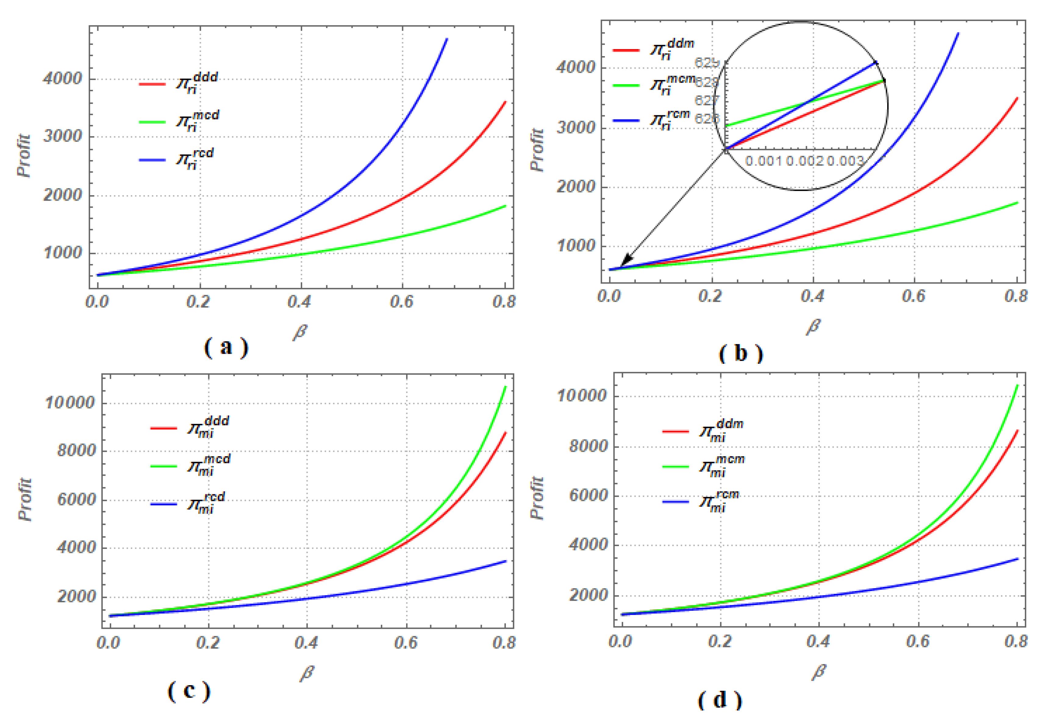
• Two manufacturers always receive less profits if the downstream retailers are integrated, because ${\pi }_{mi}^{mcd}-{\pi }_{mi}^{rcd}=\frac{4a^2{\eta }_1^2(4\beta {\eta }_1(1-{\beta }^2)+{(\beta \gamma -\delta )}^2-\beta {\gamma }^2+{\delta }^2)}{{\Delta }^{mcd}{{\Delta }^{rcd}}^2}>0$.

The ratios of the profits between retailers and manufacturers for DIGPs and MIGPs are $\frac{{\pi }_{ri}^{rcd}}{{\pi }_{mi}^{rcd}}=\frac{4{\eta }_1}{(1-\beta )(8{\eta }_1-{\gamma }^2)}$ and $\frac{{\pi }_{ri}^{rcm}}{{\pi }_{mi}^{rcm}}=\frac{1}{2(1-\beta )}$, respectively, which is almost similar with previous two game structures.

From the optimal decisions in the above three game structures, we can observe some important managerial insights. The green quality level for MIGPs is independent of $\delta$ in game structure RC, i.e., integration of two downstream retailers reduces the effect of green quality levels differentiation, which is unlike game structures DD or MC. In all three game structures, increasing market potential does not affect the profit shares. The results are not surprising because the intrinsic market potential drives the decision of overall investment on green products and the willingness of the consumer is the driving force of the installation of a costly component in each product. Moreover, investment efficiency of manufacturers for the DIGPs directly affects the profit share between members, but not MIGPs. This occurs because each manufacturer can directly compensate increasing cost by setting a higher wholesale price for MIGPs. From results of Propositions 3.1–3.6, we offer the following Theorem 1 and the detailed proof is given in Appendix D.

Theorem 1.

Optimal green quality levels, retail prices, and sales volumes in game structures DD, MC, and RC satisfy the following properties:

• For DIGPs:

  1. 

  product green quality levels satisfy the following relations:

  (i) 

  ${\theta }_i^{mcd}>max\left\{{\theta }_i^{rcd},{\theta }_i^{ddd}\right\}$ if $\beta >\frac{3(\gamma +\delta )-\sqrt{9{(\gamma -\delta )}^2+4\gamma \delta }}{4\gamma }$.

  (ii) 

  ${\theta }_i^{rcd}>max\left\{{\theta }_i^{mcd},{\theta }_i^{ddd}\right\}$ if $\beta <\frac{2\delta -\gamma }{2\gamma }$.

  (iii) 

  ${\theta }_i^{ddd}>max\left\{{\theta }_i^{mcd},{\theta }_i^{rcd}\right\}$ if $\beta \in \left(\frac{2\delta -\gamma }{2\gamma },\frac{3(\gamma +\delta )-\sqrt{9{(\gamma -\delta )}^2+4\gamma \delta }}{4\gamma }\right)$

  2. 

  retail prices are minimum in Scenario DDD, i.e., $p_i^{ddd}<min\left\{p_i^{rcd},p_i^{mcd}\right\}$ if $\beta >\frac{3\delta (\gamma -\delta )}{2({\gamma }^2-\gamma \delta +{\eta }_1)}$;

  3. 

  sales volumes are maximum in Scenario DDD i.e., $q_i^{ddd}>max\left\{q_i^{rcd},q_i^{mcd}\right\}$.

• For MIGPs:

  1. 

  product green quality levels satisfy the following relations:

  (i) 

  ${\theta }_i^{mcm}>\max \left\{{\theta }_i^{rcm},{\theta }_i^{ddm}\right\}$ if $\beta \gamma >\delta$.

  (ii) 

  ${\theta }_i^{rcm}>max\left\{{\theta }_i^{mcm},{\theta }_i^{ddm}\right\}$ if $\beta \gamma <\delta$.

  2. 

  retail prices are always minimum and sales volumes are maximum in Scenario DDM.

Theorem 1 demonstrates the following managerial insights: first, horizontal integration between upstream manufacturers or downstream retailers may reduce green quality levels for DIGPs. However, if members are maximizing their respective profits, then green quality levels will be always less for MIGPs compared to game scenarios RC ot MC. Second, for both DIGPs and MIGPs, consumers need to pay less if members of competing GSCs are interested in maximizing their respective profits. Consumers might have to pay more if members are integrated with horizontal rivals, but they can receive products at a lower quality level. Therefore, government regulatory agencies need to monitor how much consumers are affected under such deals. Graphical representations for profits for manufacturers and retailers in game structures DD, MC, and RC are presented in Figure 1. We consider $a=100$, $\gamma =0.35$, ${\eta }_1=1$, ${\eta }_2=0.1$, $\delta =0.2$, $\beta \in (0,0.8)$, for numerical illustration ([36,52]).

To some extent, it is expected that profits for both manufacturers would be higher under game structure MC whereas profits for both retailers would be higher under game structure RC. Under game structure RC, the downstream retailers have more price-setting power, consequently, they can jointly set prices that can maximize their profits. Figure 1 also demonstrates this fact. Therefore, members can strategically from collusion to ensure higher profits. It is also noticeable that if cross-price elasticity increases, then profits for every member are also increased due to the price-differentiation effect. Besides, above figure also demonstrates that if consumers’ cross-price sensitivity is too low, then the intuition might not be true for MIGPs.

3.3. Influence of Vertical Integration

In this subsection, we derive optimal decisions to explore the effect of vertical integration between two competing GSCs members.

3.3.1. Optimal Decisions in Scenarios IID and IIM

In Scenarios IID and IIM, central managers in each GSC simultaneously decide on green quality levels(${\theta }_i^z$) and retail prices ($p_i^z$) by optimizing the total profit of their respective GSCs ([13,53]) ($z=iid,iim$). Therefore, wholesale prices remain insignificant, and the optimization problems for DIGPs and MIGPs are respectively presented below:

$$\underset{(p_i^{iid},{\theta }_i^{iid})}{max}{\pi }_{ci}^{iid}=p_i^{iid}{D}_i^{iid}-{\eta }_1{{\theta }_i^{iid}}^2,(i=1,2)$$

(7)

$$\underset{(p_i^{iim},{\theta }_i^{iim})}{max}{\pi }_{ci}^{iim}=(p_i^{iim}-{\eta }_2{{\theta }_i^{iim}}^2)D_i^{iim},(i=1,2)$$

(8)

We present optimal decisions in Scenarios IID, and IIM in Proposition 7 and 8, respectively, and refer to Appendix E for the detailed derivation of the optimal decision in Scenarios IID.

Proposition 7.

Optimal decision in Scenario IID is as follows:

$p_i^{iid}=\frac{2a{\eta }_1}{{\Delta }^{iid}}$; ${\theta }_i^{iid}=\frac{a\gamma }{{\Delta }^{iid}}$; ${\pi }_{ci}^{iid}=\frac{a^2{\eta }_1(4{\eta }_1-{\gamma }^2)}{{{\Delta }^{iid}}^2}$; $Q_i^{iid}=\frac{2a{\eta }_1}{{\Delta }^{iid}}$.

Proposition 8.

Optimal decision in Scenario IIM is as follows:

$p_i^{iim}=\frac{4a{\eta }_2+\gamma (3\gamma -2\delta )}{4(2-\beta ){\eta }_2}$; ${\theta }_i^{iim}=\frac{\gamma }{2{\eta }_2}$; ${\pi }_{ci}^{iim}=\frac{{(4a{\eta }_2+\gamma (\gamma +\beta \gamma -2\delta ))}^2}{16{(2-\beta )}^2{\eta }_2^2}$; $Q_i^{iim}=\frac{4a{\eta }_2+\gamma (\gamma +\beta \gamma -2\delta )}{4(2-\beta ){\eta }_2}$

Based on Propositions 7 and 8, we made the following remarks:

• The product green quality levels are directly affected by market potential and cross-quality sensitivity of consumers for the DIGPs, but not MIGPs.
• The green quality levels of the DIGPs increase with $\beta$ and $\gamma$, and decrease with $\delta$ and ${\eta }_1$.
• The green quality levels of the MIGPs do not depend on $\beta$ or $\delta$, and are increased with $\gamma$ and decreased with ${\eta }_2$.

The nature of green quality levels remains similar to the three game structures discussed previously. Please note that the retail prices, green quality levels, sales volumes and total profits for two competing GSCs remain identical in all four decision strictures due to uniform market sizes and nature of decision sequence ([10,13,53]).

3.3.2. Optimal Decisions in Scenarios IDD and IDM

In Scenarios IDD and IDM, members of one GSC are vertically integrated by a centralized manager; however, the members of other GSCs remain decentralized. Without loss of any generality, we consider the members of the first GSC to set their respective decision variables individually by maximizing their respective profits, and the members of the second GSC are vertically integrated. Therefore, we have the following optimization problems ($z=idd,idm$):

$$\left\{\begin{array}{cc}\hfill & \underset{(p_2^z,{\theta }_2^z)}{max}{\pi }_{c2}^z+\underset{w_1^z,{\theta }_1^z}{max}{\pi }_{m1}^z\hfill \\ \hfill & \left\{\begin{array}{cc}\hfill & \underset{p_1^z}{max}{\pi }_{r1}^z\hfill \end{array}\right.\hfill \end{array}\right.$$

(9)

The sequence of decision in Scenarios IDD and IDM is described as follows:

Step 1: The manufacturer in the first GSC sets the wholesale price ($w_1^z$) and green quality of the product (${\theta }_1^z$) to maximize his profit. The centralized manager decides the retail price ($p_2^z$) and green quality level (${\theta }_2^z$) by maximizing total supply chain profit for the second GSC.

Step 2: The retailer in the first GSC decides retail price ($p_1^z$) by maximizing own profit.

Optimal decisions in Scenarios IDD and IDM are presented in Propositions 9 and 10, respectively. We refer to Appendix F for the detailed derivations of the Scenarios IDD.

Proposition 9.

Optimal decision in Scenario IDD is as follows:

$w_1^{idd}=\frac{4a{\eta }_1{\lambda }_1}{{\Delta }^{idd}}$; $p_1^{idd}=\frac{6a{\eta }_1{\lambda }_1}{{\Delta }^{idd}}$; $p_2^{idd}=\frac{4a{\eta }_1(2(4+3\beta ){\eta }_1-\gamma (\gamma +\delta ))}{{\Delta }^{idd}}$; ${\theta }_1^{idd}=\frac{a\gamma {\lambda }_1}{{\Delta }^{idd}}$; ${\theta }_2^{idd}=\frac{a(2\gamma -\beta \delta )(2(4+3\beta ){\eta }_1-\gamma (\gamma +\delta ))}{{\Delta }^{idd}}$; ${\pi }_{r1}^{idd}=\frac{4a^2{\eta }_1^2{{\lambda }_1}^2}{{{\Delta }^{idd}}^2}$; ${\pi }_{m1}^{idd}=\frac{a^2{\eta }_1(8{\eta }_1-{\gamma }^2){{\lambda }_1}^2}{{{\Delta }^{idd}}^2}$; ${\pi }_{c1}^{idd}=\frac{a^2{\eta }_1(12{\eta }_1-{\gamma }^2){{\lambda }_1}^2}{{{\Delta }^{idd}}^2}$; ${\pi }_{c2}^{idd}=\frac{a^2{\eta }_1(8(2-{\beta }^2){\eta }_1+{(2\gamma -\beta \delta )}^2){(2(4+3\beta ){\eta }_1-\gamma (\gamma +\delta ))}^2}{{{\Delta }^{idd}}^2}$; $Q_1^{idd}=\frac{2a{\eta }_1(2(4+2\beta -{\beta }^2){\eta }_1-(2\gamma -\beta \delta )(\gamma +\delta ))}{{\Delta }^{idd}}$; $Q_2^{idd}=\frac{2a(2-{\beta }^2){\eta }_1(2(4+3\beta ){\eta }_1-\gamma (\gamma +\delta ))}{{\Delta }^{idd}}$.

Proposition 10.

Optimal decision in Scenario IDM is as follows:

$w_1^{idm}=\frac{{\lambda }_2+(2-{\beta }^2)(8-5{\beta }^2){\gamma }^2}{4{\Delta }^{idm}}$; $p_1^{idm}=\frac{3{\lambda }_2+(2-{\beta }^2)(8-5{\beta }^2){\gamma }^2}{8{\Delta }^{idm}}$; $p_2^{idm}=\frac{{\lambda }_3}{4{\Delta }^{idm}}$; ${\theta }_1^{idm}=\frac{\gamma }{2{\eta }_2}$; ${\theta }_2^{idm}=\frac{2\gamma -\beta \delta }{2(2-{\beta }^2){\eta }_2}$; ${\pi }_{r1}^{idm}=\frac{{{\lambda }_2}^2}{64{{\Delta }^{idm}}^2}$; ${\pi }_{m1}^{idm}=\frac{{{\lambda }_2}^2}{32{{\Delta }^{idm}}^2}$; ${\pi }_{c1}^{idm}=\frac{3{{\lambda }_2}^2}{64{{\Delta }^{idm}}^2}$; ${\pi }_{c2}^{idm}=\frac{{((2-{\beta }^2){\lambda }_3-(8-5{\beta }^2){(2\gamma -\beta \delta )}^2)}^2}{32(2-{\beta }^2){{\Delta }^{idm}}^2}$; $Q_1^{idm}=\frac{{\lambda }_2}{8{\Delta }^{idm}}$; $Q_2^{idm}=\frac{(2-{\beta }^2){\lambda }_3-(8-5{\beta }^2){(2\gamma -\beta \delta )}^2}{8{\Delta }^{idm}}$.

Based on Propositions 9 and 10, we made the following remarks:

• The product green quality level is directly affected by market potential for the DIGPs, but not MIGPs.
• The differences between green quality levels for DIGPs and MIGPs are ${\theta }_1^{idm}-{\theta }_2^{idm}=\frac{\beta (\beta \gamma -\delta )}{2(2-{\beta }^2){\eta }_2}$ and ${\theta }_1^{idd}-{\theta }_2^{idd}=\frac{2a{\eta }_1({(2+\beta )}^2\gamma -\beta (4+3\beta )\delta )}{{\Delta }^{idd}}$, respectively.
• The green quality level of the first MIGPs is independent of $\beta$ or $\delta$, and increases with $\gamma$ and decreases with ${\eta }_2$. The green quality level of second MIGPs increase with $\beta$ and $\gamma$ and decreased with $\delta$ and ${\eta }_2$.

It is difficult to explore the properties of DIGPs analytically. However, we provide the details numerically in Section 4. In all five game structures, the green quality levels of DIGPs are different. However, green quality levels for the first MIGP remain the same in Scenarios RCM, IDM, and IIM and for the second MIGP these are the same in Scenarios IDM and DDM; and in Scenarios IIM and RCM, respectively. Therefore, the strategic decision for integrating of competing members directly affects the green quality level of products. By comparing the results in game structures II, ID, and DD, we proposed the following theorems:

Theorem 2.

Optimal green quality levels, retail prices, and sales volumes in game scenarios DD, II, and ID satisfy the following properties:

• For DIGPs:

  1. 

  products green quality levels satisfy the following relations:

  (i) 

  ${\theta }_1^{iid}>max\left\{{\theta }_1^{idd},{\theta }_1^{ddd}\right\}$;

  (ii) 

  ${\theta }_2^{idd}>max\left\{{\theta }_2^{iid},{\theta }_2^{ddd}\right\}$;

  2. 

  retail prices are minimum in Scenario IID.

  3. 

  sales volumes satisfy the following relations:

  (i) 

  $q_1^{iid}>max\left\{q_1^{idd},q_1^{ddd}\right\}$;

  (ii) 

  $q_2^{idd}>max\left\{q_2^{iid},q_2^{ddd}\right\}$;

• For MIGPs:

  1. 

  green quality levels satisfy the following relations:

  (i) 

  ${\theta }_1^{ddm}>{\theta }_1^{iim}={\theta }_1^{idm}$ if $\beta \gamma >\delta$.

  (ii) 

  ${\theta }_2^{iim}<{\theta }_2^{idm}={\theta }_2^{ddm}$ if $\beta \gamma >\delta$.

  2. 

  retail price of the product is minimum in Scenario IIM.

  3. 

  sales volume satisfy the following relations:

  (i) 

  $q_1^{iim}>max\left\{q_1^{idm},q_1^{ddm}\right\}$;

  (ii) 

  $q_2^{idm}>max\left\{q_2^{iim},q_2^{ddm}\right\}$;

We refer to Appendix G for the detailed proof. In a single-manufacturer-single-retailer supply chain setting, the effectiveness of the vertical integration is well documented in the existing literature [54,55], which might not be true under competition. The results indicate that the retail price remains lower for both types of green products if members in both GSCs are vertically integrated, but green quality level might be higher under a decentralized decision for both green product types. Therefore, consumers are benefited if the GSC members are vertically integrated. Graphical representations of the total profits for each GSC in game structures DD, II, and ID, are presented in Figure 2 to study the effect on vertical integration on profits.

Figure 2 demonstrates that optimal total profits for each GSCs in Scenarios IID or IIM can be less compared to profits obtained in the decentralized decision. Consequently, we conclude that vertical integration can generate a sub-optimal outcome from the perspective of total profits. Naturally, it is interesting to study: does performance under horizontal integration strategies outperform vertical integration strategies from the perspective of profits?

4. Model Analysis

In this section, we highlight managerial insights of the study by compering optimal decisions in the perspective of supply chain members and consumers.

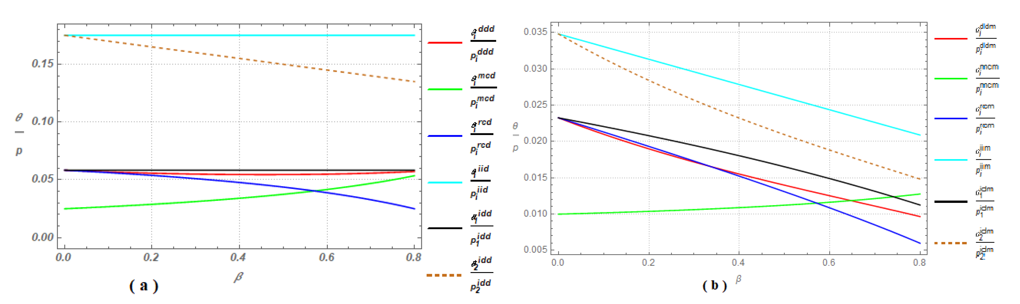
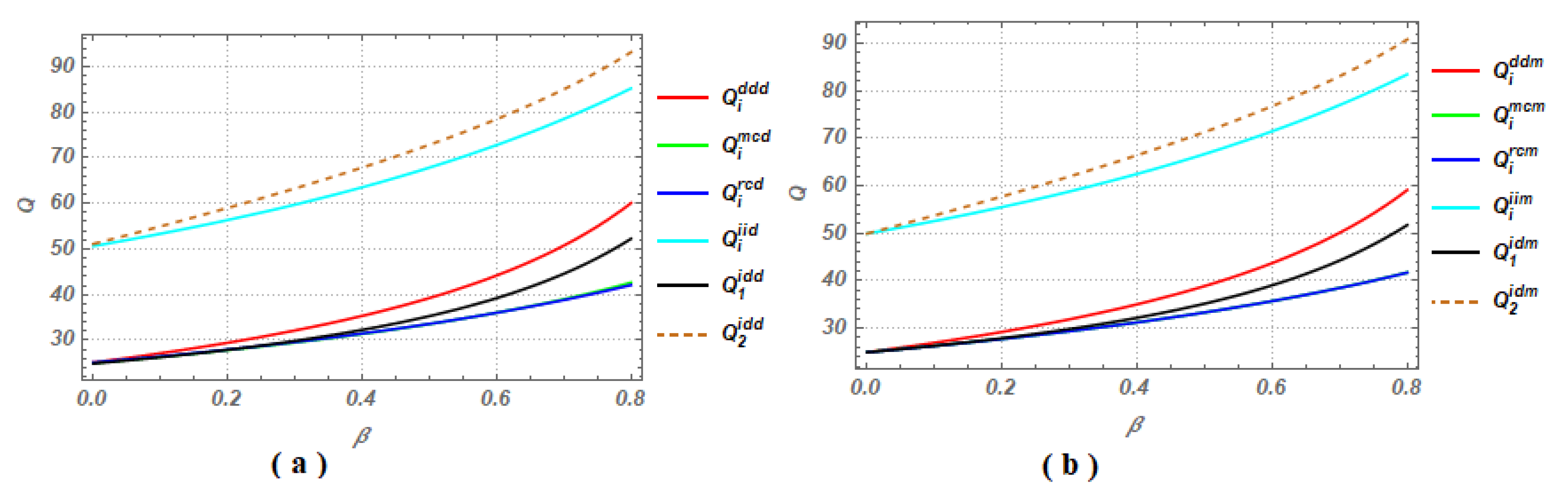
4.1. Nature of Retail Prices and Green Quality Levels under Different Scenarios

In this subsection, we explore how the parameter settings affect the retail prices and green quality levels of both product types and identify the game structure that can yield a favorable outcome for the consumers. Graphical representations of market prices and green quality levels in all scenarios are presented in Figure 3.

We observe that the green quality level may be higher in Scenario IDD and lower in Scenario RCD for DIPGs, which differs for MIGPs. However, retail prices are lower under game structure II. One point is clear, if competing members are strategically integrated, then customers might need to pay more for lower quality products. GSC members agreed on strategic integration with competitors or with their business partners to achieve business goals such as greater control for their decisions, maximize profits, improve product quality, etc. For instance, manufacturers always want to have greater control over their investment decision or retailers want more flexibility to set their respective market prices. In this circumstance, if the retailer sets higher prices, upstream manufacturers reduce the investment in green technology due to lower demand, the results are reflect this fact. To obtain deeper insights on this issue, we draw the following figure that represents the ratios of green quality levels and prices $\frac{{\theta }_i^s}{p_i^s}$ to demonstrate a comparative overview of how much consumers need to pay for green quality levels under different scenarios.

Figure 4 provides the following notable insights: (i) the ratio of $\frac{{\theta }_i^s}{p_i^s}$ is higher in Scenarios IID or IIM, consequently, strategic integration with vertical members always leads to a favorable outcome for consumers, especially those whose expenditure is driven by what quality they are receiving; (ii) the ratio appears to be lower in game structures MC or RC, therefore, horizontal integration, especially at downstream level, hurts consumers.

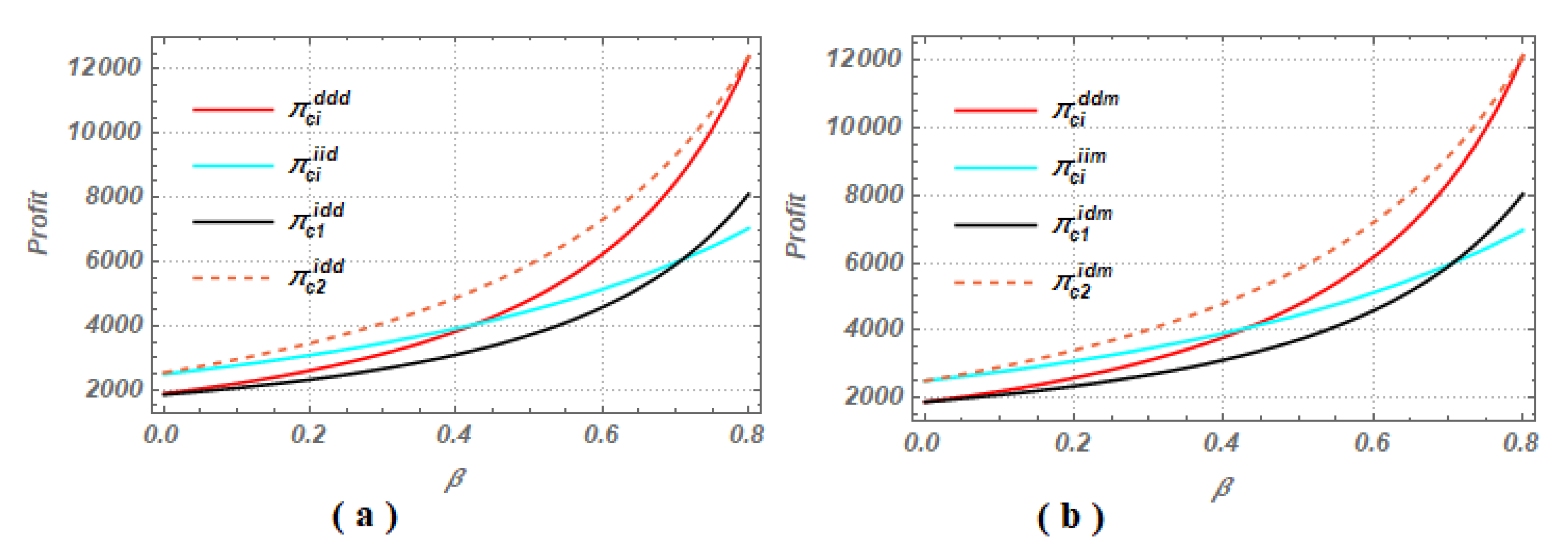
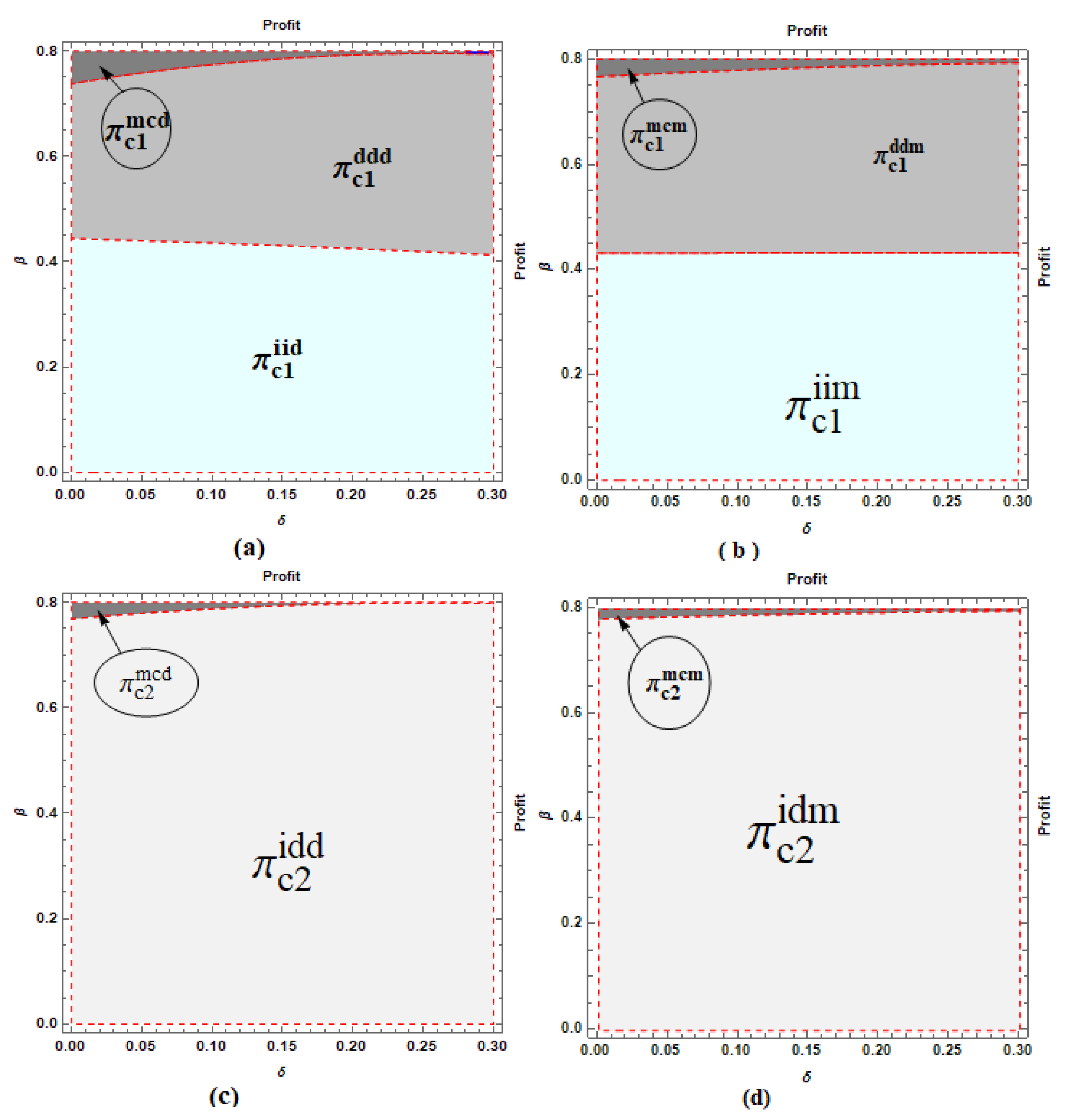
4.2. Nature of Sales Volumes and Profits for Two Competing GSCs

Now we compare the sales volume of two GSCs under different game structures, and the corresponding graphical representation is presented in Figure 5.

Figure 5 demonstrates that sales volumes are less for both product types when members are horizontally integrated. Please note that retail prices are higher and green quality level is lower when members are horizontally integrated. Therefore, the results make sense. If the consumers need to pay more for lower quality products, then the demand decreases. Therefore, horizontal integration can potentially reduce green product consumption for both product types. Finally, we compare the total profits for two competing GSCs.

Figure 6 demonstrates the following key outcomes: (i) in manufacturers dominated GSCs, it is expected that total profits for both GSCs under strategic integration between two retailers may degrade the overall performance of GSCs. The results also reflect this fact. Therefore, we conclude downstream integration might hurt GSC members. (ii) For both types of products, horizontal integration between two manufacturers, decentralized decision, or vertical integration may lead to maximum profits. If cross-price elasticity is higher, then vertical integration is not an optimal option for the competing GSCs. Although in single-retailer-single-manufacturer GSCs, the total profits supply chain is always maximum if members are vertically integrated, (iii) it is expected that if the members in the first competing GSC are decentralized, members in the second GSC are integrated by centralized managers, then total profits for second GSC will be always higher. The results also reflect this fact. However, there are some market parameter settings, where integration between two upstream manufacturers can lead to a favorable outcome. (iv) Because, the dominating regions are not uniform, therefore, green product types influence the strategic integration decision.

Therefore, members in the competing GSCs face the Prisoner’s dilemma. Through horizontal integration, they can achieve the profit maximization objective, but they need to trade lower quality product. Supply chain managers need to carefully decide the strategic option for integration by taking into account the product type before selecting such strategic measures. Please note that if $\gamma =0$ and $\delta =0$, i.e., both manufacturers trade with normal products, then the total profits in five scenarios satisfy the following relations:

Theorem 3.

If the manufacturers trade with normal products, the total profits for each supply chain satisfy the following relations:

• Total profits for first GSC satisfy the following relation:
  • ${\pi }_{c1}^{ii}>{\pi }_{c1}^{dd}>{\pi }_{c1}^{mc}={\pi }_{c1}^{rc}>{\pi }_{c1}^{id}$ if $\beta <0.43$
  • ${\pi }_{c1}^{dd}>{\pi }_{c1}^{ii}>{\pi }_{c1}^{mc}={\pi }_{c1}^{rc}>{\pi }_{c1}^{id}$ if $0.43<\beta <0.5$
  • ${\pi }_{c1}^{dd}>{\pi }_{c1}^{mc}={\pi }_{c1}^{rc}>{\pi }_{c1}^{ii}>{\pi }_{c1}^{id}$ if $0.5<\beta <0.7$
  • ${\pi }_{c1}^{dd}>{\pi }_{c1}^{mc}={\pi }_{c1}^{rc}>{\pi }_{c1}^{id}>{\pi }_{c1}^{ii}$ if $0.7<\beta <0.8$
• Total profits for second GSC satisfy the following relation:
  • ${\pi }_{c2}^{id}>{\pi }_{c2}^{ii}>{\pi }_{c2}^{dd}>{\pi }_{c2}^{mc}={\pi }_{c2}^{rc}$ if $\beta <0.43$
  • ${\pi }_{c2}^{id}>{\pi }_{c2}^{dd}>{\pi }_{c2}^{ii}>{\pi }_{c2}^{mc}={\pi }_{c2}^{rc}$ if $0.43<\beta <0.5$
  • ${\pi }_{c2}^{id}>{\pi }_{c2}^{dd}>{\pi }_{c2}^{mc}={\pi }_{c2}^{rc}>{\pi }_{c1}^{ii}$ if $0.5<\beta <0.8$

Please note that if the demand function is price sensitive only, the investment decision does not make any impact on the profits. Theorem 3 demonstrates that except cross-price elasticity is too high, total supply chain profits always higher in game structures DD, ID, or II (Please see Appendix I).

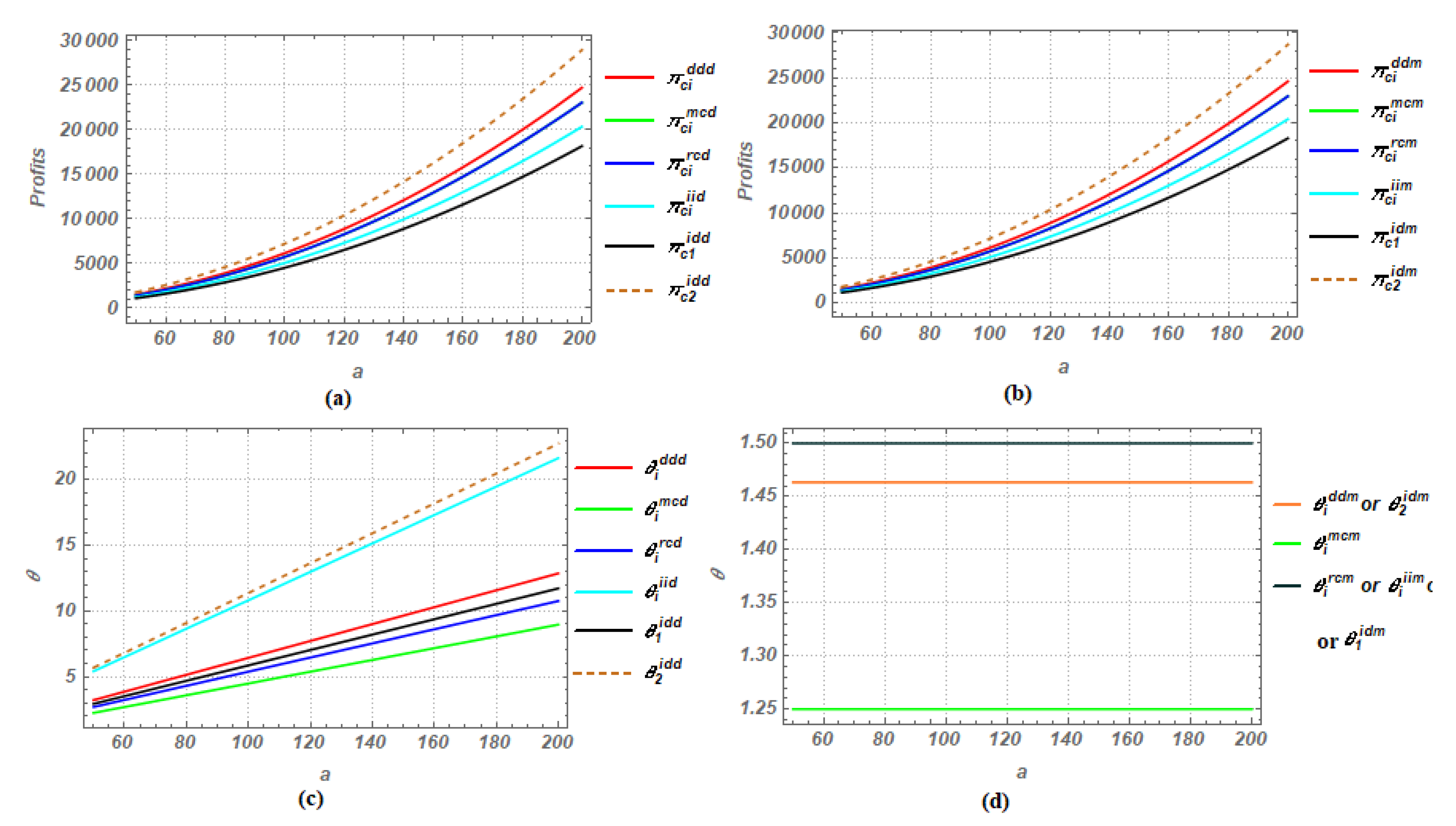
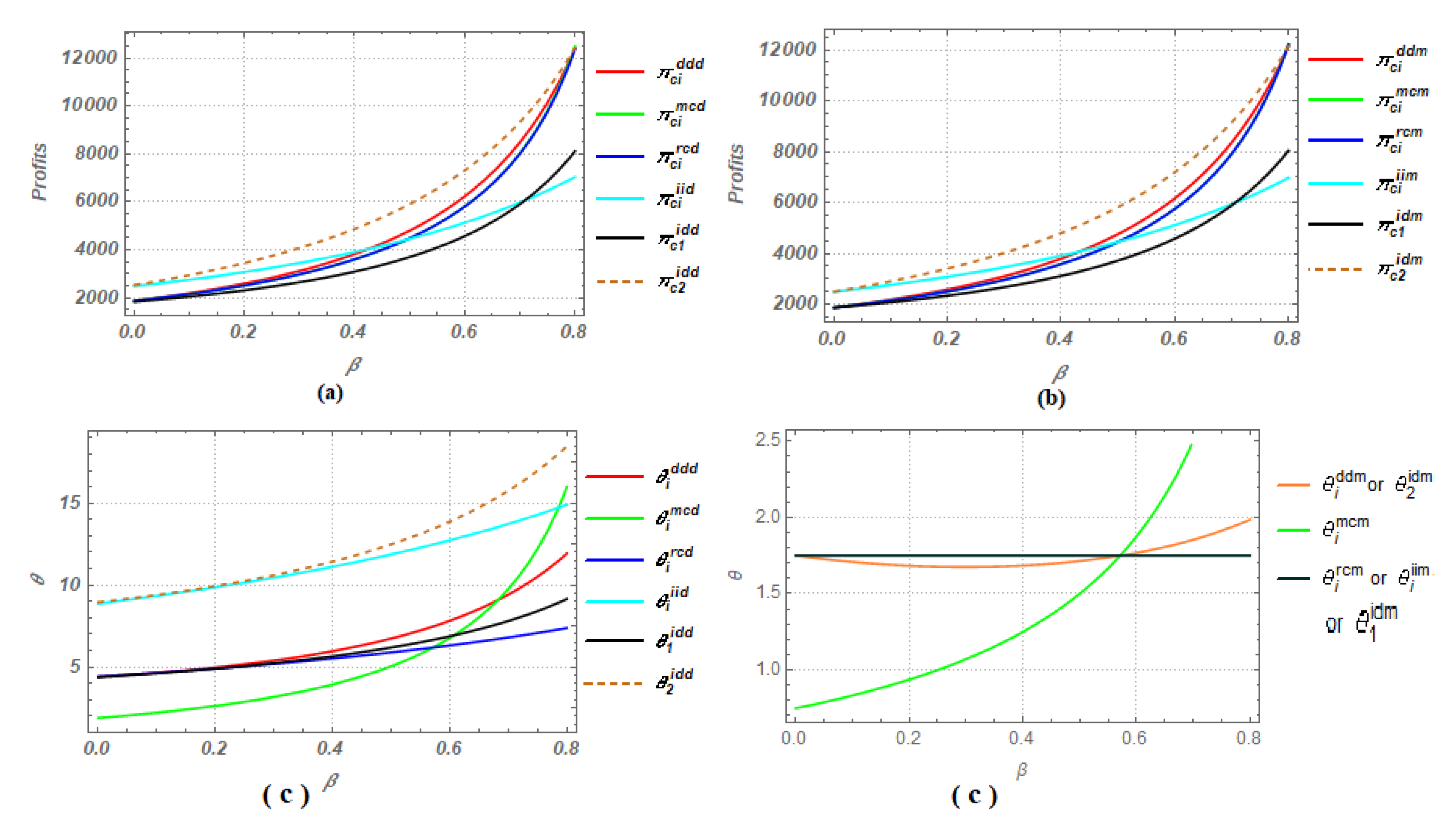
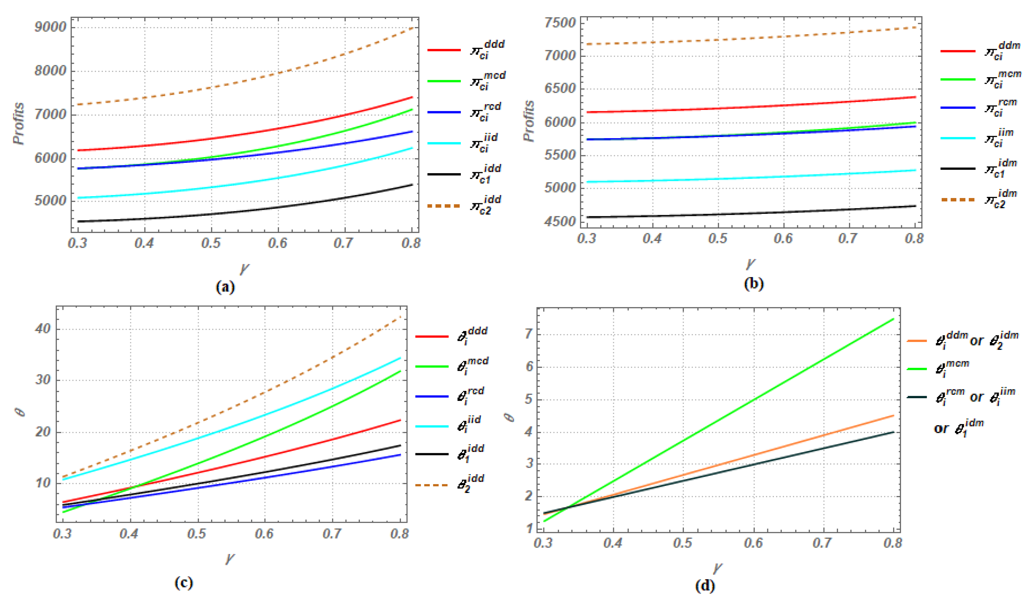
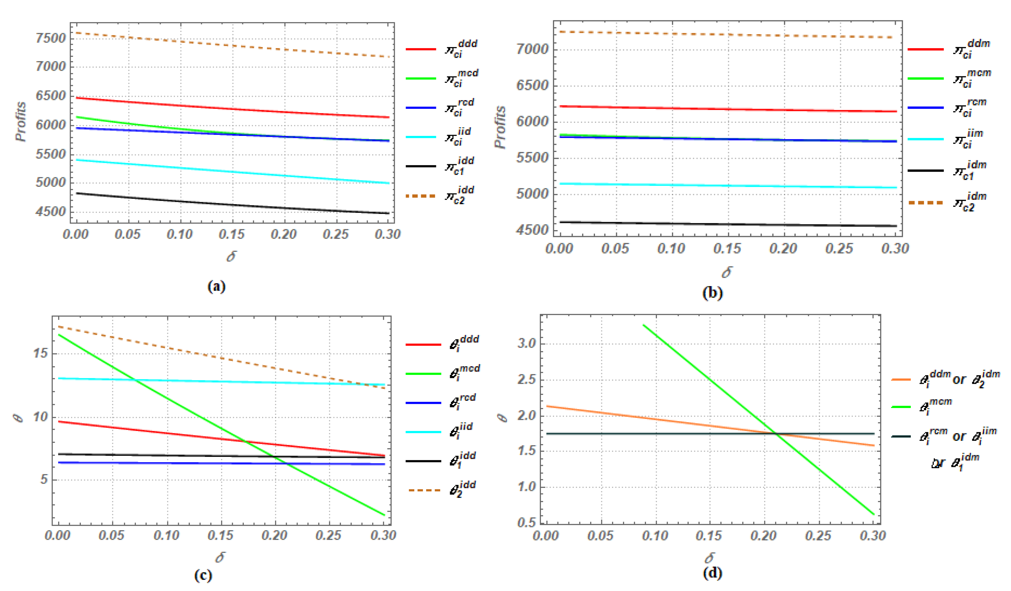
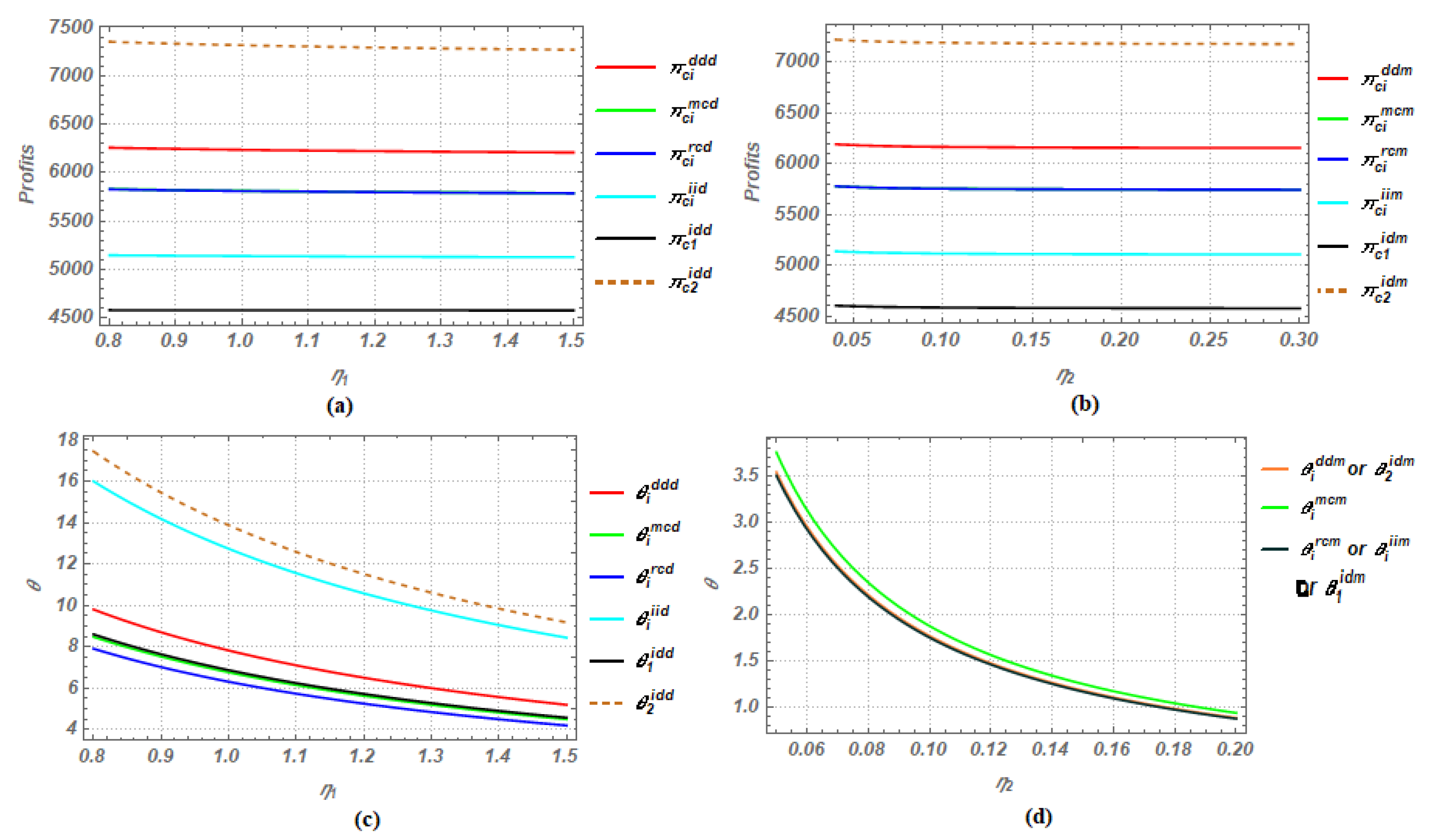
4.3. Effect of Parameters on the Optimal Performance

Because it is difficult to establish an analytical relationship among total GSC profits for DIGPs and MIGPs, we conduct a sensitivity analysis for green quality levels and total profits with respect to each parameter by keeping other parameters as fixed. The detailed results are presented below in

Table 3. Characteristics of green quality levels and total GSC profits for DIGPs.

Parameters	GSC	Green Quality Level for DIGPs	Total GSC Profits
$a\in (50,200)$	I	$II>MC>DD>ID>RC$	$DD>MC>RC>II>ID$
	$II$	$ID>II>MC>DD>RC$	$ID>DD>MC>RC>II$
$\beta \in (0,0.8)$	I	$II>DD>RC>ID>MC$ if $\beta \in (0,0.3)$	$II>DD>RC>MC>ID$ if $\beta \in (0,0.43)$
		$II>DD>ID>RC>MC$ if $\beta \in (0.3,0.56)$	$DD>II>MC>RC>ID$ if $\beta \in (0.43,0.5)$
		$II>DD>ID>MC>RC$ if $\beta \in (0.56,0.62)$	$DD>MC>RC>II>ID$ if $\beta \in (0.5,0.71)$
		$II>DD>MC>ID>RC$ if $\beta \in (0.62,0.71)$	$DD>MC>RC>ID>II$ if $\beta \in (0.71,0.76)$
		$II>MC>DD>ID>RC$ if $\beta \in (0.71,0.78)$	$MC>DD>RC>ID>II$ if $\beta \in (0.76,0.8)$
		$MC>II>DD>ID>RC$ if $\beta \in (0.78,0.8)$
	$II$	$ID>II>DD>RC>MC$ if $\beta \in (0,0.56)$	$ID>II>DD>RC>MC$ if $\beta \in (0,0.43)$
		$ID>II>DD>MC>RC$ if $\beta \in (0.56,0.71)$	$ID>DD>II>MC>RC$ if $\beta \in (0.43,0.5)$
		$ID>II>MC>DD>RC$ if $\beta \in (0.71,0.78)$	$ID>DD>MC>RC>II$ if $\beta \in (0.5,0.76)$
		$ID>MC>II>DD>RC$ if $\beta \in (0.78,0.8)$	$MC>ID>DD>RC>II$ if $\beta \in (0.76,0.8)$
$\gamma \in (0.3,0.8)$	I	$II>DD>ID>RC>MC$ if $\gamma \in (0.3,0.34)$	$DD>MC>RC>II>ID$
		$II>DD>ID>MC>RC$ if $\gamma \in (0.34,0.37)$	if $\gamma \in (0.3,0.32)\bigcup (0.39,0.8)$
		$II>DD>MC>ID>RC$ if $\gamma \in (0.37,0.42)$	$DD>RC>MC>II>ID$ if $\gamma \in (0.32,0.39)$
		$II>MC>DD>ID>RC$ if $\gamma \in (0.42,0.8)$
	$II$	$ID>II>DD>RC>MC$ if $\gamma \in (0.3,0.34)$	$ID>DD>MC>RC>II$
		$ID>II>DD>MC>RC$ if $\gamma \in (0.34,0.41)$	if $\gamma \in (0.3,0.32)\bigcup (0.39,0.8)$
		$ID>II>MC>DD>RC$ if $\gamma \in (0.41,0.8)$	$ID>DD>RC>MC>II$ if $\gamma \in (0.31,0.39)$
$\delta \in (0,0.3)$	I	$MC>II>DD>ID>RC$ if $\delta \in (0,0.06)$	$DD>MC>RC>II>ID$
		$II>MC>DD>ID>RC$ if $\delta \in (0.06,0.14)$	if $\delta \in (0,0.16)\bigcup (0.21,0.3)$
		$II>DD>MC>ID>RC$ if $\delta \in (0.14,0.16)$	$DD>RC>MC>II>ID$if $\delta \in (0.16,0.21)$
		$II>DD>ID>MC>RC$ if $\delta \in (0.16,0.18)$
		$II>DD>ID>RC>MC$ if $\delta \in (0.18,0.3)$
	$II$	$ID>MC>II>DD>RC$ if $\delta \in (0,0.06)$	$ID>DD>MC>RC>II$
		$ID>II>MC>DD>RC$ if $\delta \in (0.06,0.14)$	if $\delta \in (0,0.16)\bigcup (0.21,0.3)$
		$ID>II>DD>MC>RC$ if $\delta \in (0.14,0.18)$	$ID>DD>RC>MC>II$ if $\delta \in (0.21,0.3)$
		$ID>II>DD>RC>MC$ if $\delta \in (0.18,0.24)$
		$II>ID>DD>RC>MC$ if $\delta \in (0.24,0.3)$
${\eta }_1\in (0.8,1.5)$	I	$II>DD>ID>MC>RC$	$DD>MC>RC>II>ID$
	$II$	$ID>II>DD>MC>RC$	$ID>DD>MC>RC>II$

and

Table 4. Characteristics of green quality levels and total GSC profits for MIGPs.

Parameter	GSC	Green Quality Level for MIGPs	Total GSC Profits
$a\in (200,500)$	I	$MC>DD>RC=II=ID$	$DD>MC>RC>II>ID$
	$II$	$MC>DD=ID>RC=II$	$ID>DD>MC>RC>II$
$\beta \in (0,0.8)$	I		$II>DD>RC>MC>ID$ if $\beta \in (0,0.43)$
		$RC=II=ID>DD>MC$ if $\beta \in (0,0.56)$	$DD>II>MC>RC>ID$ if $\beta \in (0.43,0.5)$
		$MC>DD>RC=II=ID$ if $\beta \in (0.56,0.8)$	$DD>MC>RC>II>ID$ if $\beta \in (0.5,0.7)$
			$DD>MC>RC>ID>II$ if $\beta \in (0.7,0.8)$
	$II$	$RC=II>DD=ID>MC$ if $\beta \in (0,0.56)$	$ID>II>DD>RC>MC$ if $\beta \in (0,0.43)$
		$MC>DD=ID>RC=II$ if $\beta \in (0.56,0.8)$	$ID>DD>II>MC>RC$ if $\beta \in (0.43,0.5)$
			$ID>DD>MC>RC>II$ if $\beta \in (0.5,0.8)$
$\gamma \in (0.3,0.8)$	I	$RC=II=ID>DD>MC$ if $\gamma \in (0.3,0.34)$
		$MC>DD>RC=II=ID$ if $\gamma \in (0.34,0.8)$	$DD>MC>RC>II>ID$
	$II$	$RC=II>DD=ID>MC$ if $\gamma \in (0.3,0.34)$	$ID>DD>MC>RC>II$
		$MC>DD=ID>RC=II$ if $\gamma \in (0.34,0.8)$
$\delta \in (0,0.3)$	I	$MC>DD>RC=II=ID$ if $\delta \in (0,0.18)$
		$RC=II=ID>DD>MC$ if $\delta \in (0.18,0.3)$	$DD>MC>RC>II>ID$
	$II$	$MC>DD=ID>RC=II$ if $\delta \in (0,0.18)$	$ID>DD>MC>RC>II$
		$RC=II>DD=ID>MC$ if $\delta \in (0.18,0.3)$
${\eta }_2\in (0.01,0.2)$	I	$MC>DD>RC=II=ID$	$DD>MC>RC>II>ID$
	$II$	$MC>DD=ID>RC=II$	$ID>DD>MC>RC>II$

. We present the detail in Appendix K.

It is observed that green quality levels and profits of GSC members increase with the increasing values of a, $\gamma$, and $\beta$; and the reverse trend is found for ${\eta }_i$ and $\delta$. As overall intrinsic market demand increases, profit subsequently increases. In these circumstances, both manufacturers have a higher flexibility in investment to improve green product quality. Similarly, if consumers are sensitive to green quality levels, demand for the products increases and total profit for each GSC also increased. It is expected that profits of each GSC decreased with the increment of ${\eta }_i$, in that scenario both manufacturers need to invest more. However, the main insights from the analysis are listed below:

• If the product is price sensitive only, total supply chain profits can never be maximum if two upstream manufacturers are integrated, which is not true while they are trading with green products.
• Similar to normal products, cross-price elasticity is an important factor affecting strategic integration decisions from the perspective of profits. In addition, $\gamma$ and $\delta$ also affect the strategic decision. Therefore, a careful estimation of parameters and strategic integration decisions can bring higher profits for the GSC members, but not always. It is found that each member can receive a higher profit when they are non-cooperative.
• For MIGPs, green quality levels are higher in game structures MC or MC, but for DIGPs these are higher in game structures II and ID. Most interestingly, total profits for MIGPs are higher in game structures II, ID or DD. Therefore, GSC members need to sacrifice one of their goals, i.e., trading with higher quality green products to ensure environmental sustainability or profit maximization.

5. Conclusions

In this study, we explore the strategic integration and investment decisions for two competing GSC members by taking into consideration two green product types, namely DIGPs and MIGPs. In the existing literature, comparative study on DIGPs and MIGPs under supply chain competition is limited. To address the problem, we formulate five game-theoretic models by assuming each manufacturer sells substitutable products through exclusive retailers, and investigate price and green quality decisions. We compare prices, green quality levels, and profits for both types of products; and the following key insights are obtained that can offer insightful recommendations regarding GSC practice under the competition. First, strategic integration decisions with competing manufacturers can be proven to be a potential choice for value-added sustainable product development strategy. In that scenario, total profits for each GSC can be higher compared to the profits obtained under horizontal integration. However, a strategic integration decision for two retailers not only hurts green quality levels of products, but it also causes lower profits for both GSCs; similar results also reported in the literature where the authors consider only price dependent demand ([13]). Second, supply chain managers need to examine the market-related parameters associated with green product types before exercising horizontal or vertical strategic choice of integration. The comparative analysis yields a clear-cut result that under competition vertical integration among GSC members does not necessarily yield maximum profit, which is completely the opposite to that found in single-manufacturer-single-retailer supply chain decisions. Each member can receive higher profits even under decentralized decision structures. Third, while trading with green products under competition, GSC members might have to sacrifice one of their business goals, i.e., trading with higher quality products to ensure environmental sustainability or profit maximization. Finally, this research into environmental monitoring agencies only needs to consider the possible strategic alliance among competitors while making regulations.

The present study demonstrates that total profits for both competing GSCs might be maximized if members are horizontally integrated. Therefore, as future research, one possible area of study is the effect of information asymmetry and the effects of demand uncertainty while two competing manufacturers are horizontally integrated. In our study, we have ignored the effect of cross-channel selling; consequently, it will be interesting to explore the characteristics of the optimal decisions in the presence of another degree of competition. The effect of government subsidy or tax on GSCs has been a topic of interest over the last couple of years. Therefore, it would be interesting to study the effects of subsidies or tax on green supply chain members, or direct subsidy to consumers under competition. Presently, many consumers prefers to buy product through online channel, therefore, it will be interesting to derive results in the presence of an online channel and study the strategic preference for competing supply chain members [56,57]. Finally, one can study the impact of horizontal cooperation with multiple members of players at each echelon.

References

1. Yang, Z.; Lin, Y. The effects of supply chain collaboration on green innovation performance: An interpretive structural modeling analysis. Sustain. Prod. Consum. 2020, 23, 1–10. [Google Scholar] [CrossRef]
2. Hasan, M.M.; Nekmahmud, M.; Yajuan, L.; Patwary, M.A. Green business value chain: A systematic review. Sustain. Prod. Consum. 2019, 20, 326–339. [Google Scholar] [CrossRef]
3. Liu, X.; Lin, K.; Wang, L.; Ding, L. Pricing decisions for a sustainable supply chain in the presence of potential strategic customers. Sustainability 2020, 12, 1655. [Google Scholar] [CrossRef] [Green Version]
4. Businesswire. More Than Half of Consumers would Pay More for Sustainable Products Designed to be Reused or Recycled, Accenture Survey Finds. 2019. Available online: www.businesswire.com/news/home/20190604005649/en (accessed on 6 June 2020).
5. Jasiulewicz-Kaczmarek, M.; Legutko, S.; Kluk, P. Maintenance 4.0 technologies—New opportunities for sustainability driven maintenance. Manag. Prod. Eng. Rev. 2020, 11, 74–87. [Google Scholar]
6. Tumpa, T.J.; Ali, S.M.; Rahman, M.H.; Paul, S.K.; Chowdhury, P.; Khan, S.A.R. Barriers to green supply chain management: An emerging economy context. J. Clean. Prod. 2019, 236, 117617. [Google Scholar] [CrossRef]
7. Wang, J.; Chang, J.; Wu, Y. The optimal production decision of competing supply chains when considering green degree: A game-theoretic approach. Sustainability 2020, 12, 7413. [Google Scholar] [CrossRef]
8. Wang, S.; Cheng, Y.; Zhang, X.; Zhu, C. The implications of vertical strategic interaction on green technology investment in a supply chain. Sustainability 2020, 12, 7441. [Google Scholar] [CrossRef]
9. Wei, J.; Zhao, J.; Hou, X. Integration strategies of two supply chains with complementary products. Int. J. Prod. Res. 2019, 57, 1972–1989. [Google Scholar] [CrossRef]
10. Bian, J.; Zhao, X.; Liu, Y. Single vs. cross distribution channels with manufacturers’ dynamic tacit collusion. Int. J. Prod. Econ. 2020, 220, 107456. [Google Scholar] [CrossRef]
11. Garrett, B. Why Collaborating with Your Competition Can Be A Great Idea. 2019. Available online: www.forbes.com/sites/briannegarrett/2019/09/19/why-collaborating-with-your-competition-can-be-a-great-idea/#3cd85f8ddf86 (accessed on 2 October 2020).
12. Colombo, S. Mixed oligopolies and collusion. J. Econ. 2016, 118, 167–184. [Google Scholar] [CrossRef]
13. Zhou, Y.W.; Cao, Z.H. Equilibrium structures of two supply chains with price and displayed-quantity competition. J. Oper. Res. Soc. 2014, 65, 1544–1554. [Google Scholar] [CrossRef]
14. Lambertini, L.; Orsini, R.; Palestini, A. On the instability of the R&D portfolio in a dynamic monopoly. Or, one cannot get two eggs in one basket. Int. J. Prod. Econ. 2017, 193, 703–712. [Google Scholar]
15. Li, Q.; Guan, X.; Shi, T.; Jiao, W. Green product design with competition and fairness concerns in the circular economy era. Int. J. Prod. Res. 2020, 58, 165–179. [Google Scholar] [CrossRef]
16. Wang, Y.; Wang, X.; Chang, S.; Kang, Y. Product innovation and process innovation in a dynamic Stackelberg game. Comput. Ind. Eng. 2019, 130, 395–403. [Google Scholar] [CrossRef]
17. Dey, K.; Roy, S.; Saha, S. The impact of strategic inventory and procurement strategies on green product design in a two-period supply chain. Int. J. Prod. Res. 2019, 57, 1915–1948. [Google Scholar] [CrossRef]
18. Zhu, W.; He, Y. Green product design in supply chains under competition. Eur. J. Oper. Res. 2017, 258, 165–180. [Google Scholar] [CrossRef]
19. Qian, L. Product price and performance level in one market or two separated markets under various cost structures and functions. Int. J. Prod. Econ. 2011, 131, 505–518. [Google Scholar] [CrossRef]
20. Chang, S.; Hu, B.; He, X. Supply chain coordination in the context of green marketing efforts and capacity expansion. Sustainability 2019, 11, 5734. [Google Scholar] [CrossRef] [Green Version]
21. Choi, S.C. Price competition in a duopoly common retailer channel. J. Retail. 1996, 72, 117–134. [Google Scholar] [CrossRef]
22. Ha, A.Y.; Tong, S. Contracting and Information Sharing Under Supply Chain Competition. Manag. Sci. 2008, 54, 701–715. [Google Scholar] [CrossRef]
23. Moorthy, K.S. Strategic decentralization in channels. Mark. Sci. 1988, 7, 335–355. [Google Scholar] [CrossRef]
24. Anderson, E.J.; Bao, Y. Price competition with integrated and decentralized supply chains. Eur. J. Oper. Res. 2010, 200, 227–234. [Google Scholar] [CrossRef]
25. Li, B.X.; Zhou, Y.; Li, J.; Zhou, S. Contract choice game of supply chain competition at both manufacturer and retailer levels. Int. J. Prod. Econ. 2013, 143, 188–197. [Google Scholar] [CrossRef]
26. Fang, Y.; Shoub, B. Managing supply uncertainty under supply chain Cournot competition. Eur. J. Oper. Res. 2015, 243, 156–176. [Google Scholar] [CrossRef]
27. Xie, G. Modeling decision processes of a green supply chain with regulation on energy saving level. Comput. Oper. Res. 2015, 54, 266–273. [Google Scholar] [CrossRef]
28. Bian, W.; Shang, J.; Zhang, J. Two-way information sharing under supply chain competition. Int. J. Prod. Econ. 2016, 178, 82–94. [Google Scholar] [CrossRef]
29. Li, X.; Li, Y. Chain-to-chain competition on product sustainability. J. Clean. Prod. 2016, 112, 2058–2065. [Google Scholar] [CrossRef]
30. Wang, Y.Y.; Sun, J.; Wang, J.C. Equilibrium markup pricing strategies for the dominant retailers under supply chain to chain competition. Int. J. Prod. Res. 2016, 54, 2075–2092. [Google Scholar] [CrossRef]
31. Hafezalkotob, A. Competition, cooperation, and coopetition of green supply chains under regulations on energy saving levels. Transp. Res Part E 2017, 97, 228–250. [Google Scholar] [CrossRef]
32. Hafezalkotob, A. Modelling intervention policies of government in price-energy saving competition of green supply chains. Comput. Ind. Eng. 2018, 119, 247–261. [Google Scholar] [CrossRef]
33. Xiao, T.; Yang, D. Price and service competition of supply chains with risk-averse retailers under demand uncertainty. Int. J. Prod. Econ. 2008, 114, 187–200. [Google Scholar] [CrossRef]
34. Li, G.; Shi, X.; Yang, Y.; Lee, P.K. Green Co-Creation Strategies among Supply Chain Partners: A Value Co-Creation Perspective. Sustainability. 2020, 12, 4305. [Google Scholar] [CrossRef]
35. Lin, Y.H.; Kulangara, N.; Foster, K.; Shang, J. Improving green market orientation, green supply chain relationship quality, and green absorptive capacity to enhance green competitive advantage in the green supply chain. Sustainability 2020, 12, 7251. [Google Scholar] [CrossRef]
36. Saha, S.; Majumder, S.; Nielsen, I.E. Is it a strategic move to subsidized consumers instead of the manufacturer? IEEE Access 2019, 7, 169807–169824. [Google Scholar] [CrossRef]
37. Basiri, Z.; Heydari, J. A mathematical model for green supply chain coordination with substitutable products. J. Clean. Prod. 2017, 145, 232–249. [Google Scholar] [CrossRef] [Green Version]
38. Dey, K.; Saha, S. Influence of procurement decisions in two-period green supply chain. J. Clean. Prod. 2018, 190, 388–402. [Google Scholar] [CrossRef]
39. Ghosh, D.; Shah, J. Supply chain analysis under green sensitive consumer demand and cost sharing contract. Int. J. Prod. Econ. 2015, 164, 319–329. [Google Scholar] [CrossRef]
40. Li, Q.; Kang, Y.; Tan, L.; Chen, B. Modeling formation and operation of collaborative green innovation between manufacturer and supplier: A game theory approach. Sustainability 2020, 12, 2209. [Google Scholar] [CrossRef] [Green Version]
41. Liu, P.; Yi, S.P. Pricing policies of green supply chain considering targeted advertising and product green degree in the big data environment. J. Clean. Prod. 2017, 164, 1614–1622. [Google Scholar] [CrossRef]
42. Nielsen, I.E.; Majumder, S.; Sana, S.S.; Saha, S. Comparative analysis of government incentives and game structures on single and two-period green supply chain. J. Clean. Prod. 2019, 235, 1371–1398. [Google Scholar] [CrossRef]
43. Song, H.; Gao, X. Green supply chain game model and analysis under revenue-sharing contract. J. Clean. Prod. 2018, 170, 183–192. [Google Scholar] [CrossRef]
44. Yang, D.; Xiao, T. Pricing and green level decisions of a green supply chain with governmental interventions under fuzzy uncertainties. J. Clean. Prod. 2017, 149, 1174–1187. [Google Scholar] [CrossRef]
45. Chakrabortya, T.; Chauhana, S.S.; Ouhimmou, M. Cost-sharing mechanism for product quality improvement in a supply chain under competition. Int. J. Prod. Econ. 2019, 208, 566–587. [Google Scholar] [CrossRef]
46. Nielsen, I.E.; Majumder, S.; Saha, S. Exploring the intervention of intermediary in a green supply chain. J. Clean. Prod. 2019, 233, 1525–1544. [Google Scholar] [CrossRef]
47. Li, T.; Zhang, R.; Zhao, S.; Liu, B. Low carbon strategy analysis under revenue-sharing and cost-sharing contracts. J. Clean. Prod. 2019, 212, 1462–1477. [Google Scholar] [CrossRef]
48. Zhou, Y. The role of green customers under competition: A mixed blessing? J. Clean. Prod. 2018, 170, 857–866. [Google Scholar] [CrossRef]
49. Gao, J.; Xiao, Z.; Wei, H.; Zhou, G. Dual-channel Green Supply Chain Management with Eco-label Policy: A Perspective of Two Types of Green Products. Comput. Ind. Eng. 2020, 146, 106613. [Google Scholar] [CrossRef]
50. Pakseresht, M.; Shirazi, B.; Mahdavi, I.; Mahdavi-Amiri, N. Toward sustainable optimization with Stackelberg game between green product family and downstream supply chain. Sustain. Prod. Consum. 2020, 23, 198–211. [Google Scholar] [CrossRef]
51. Reinartz, W.; Wieg, N.; Imschloss, M. The impact of digital transformation on the retailing value chain. Int. J. Res. Mark. 2019, 36, 350–366. [Google Scholar] [CrossRef]
52. Yang, S.; Ding, P.; Wang, G.; Wu, X. Green investment in a supply chain based on price and quality competition. Soft Comput. 2020, 24, 2589–2608. [Google Scholar] [CrossRef]
53. Wei, J.; Lu, J.; Zhao, J. Interactions of competing manufacturers’ leader-follower relationship and sales format on online platforms. Eur. J. Oper. Res. 2020, 280, 508–522. [Google Scholar] [CrossRef]
54. Cachon, G.P. Supply chain coordination with contracts. Handb. Oper. Res. Manag. Sci. 2003, 11, 227–339. [Google Scholar]
55. Li, X.; Wang, Q. Coordination mechanisms of supply chain systems. Eur. J. Oper. Res. 2007, 179, 1–16. [Google Scholar] [CrossRef]
56. Qiongqiong, G.; Xiaodong, Y.; Bin, L. Pricing Decisions on Online Channel Entry for Complementary Products in a Dominant Retailer Supply Chain. Sustainability 2020, 12, 5007. [Google Scholar] [CrossRef]
57. Saha, S.; Sarmah, S.P.; Moon, I. Dual channel closed-loop supply chain coordination with a reward-driven remanufacturing policy. Int. J. Prod. Res. 2016, 54, 1503–1517. [Google Scholar] [CrossRef]
Figure 1. Profits of retailers for (a) DIGPs and (b) MIGPs; and profits of manufacturers for (c) DIGPs and (d) MIGPs.
Sustainability 12 10248 g001
Figure 2. Total profits for each GSC for (a) for DIGPs and (b) MIGPs.
Sustainability 12 10248 g002
Figure 3. Retail prices for (a) DIGPs and (b) MIGPs; and green quality levels for (c) DIGPs and (d) for MIGPs under different game structures.
Sustainability 12 10248 g003
Figure 4. Ratios of green quality levels with retail prices for (a) DIGPs and (b) MIGPs under different game structures.
Sustainability 12 10248 g004
Figure 5. Sales volumes for (a) DIGPs and (b) MIGPs, under different game structures.
Sustainability 12 10248 g005
Figure 6. Profits for (a) first GSC for DIGPs, (b) first GSC for MIGPs, (c) second GSC for DIGPs, (d) second GSC for MIGPs, under different game structures.
Sustainability 12 10248 g006