Development of a Soil Quality Index for Soils under Different Agricultural Management Conditions in the Central Lowlands of Mexico: Physicochemical, Biological and Ecophysiological Indicators

Abstract

The Bajío—Mexico’s central lowlands—is a region of economic importance because of its agricultural industry. Over time, agricultural practices have led to soil deterioration, loss of fertility, and abandonment. In this study, six agricultural soils were analyzed: AGQ, CTH, CTJ, JRM, CRC, and CYI, and used to develop a soil quality index (SQI) that includes the use of physicochemical, biological, and ecophysiological indicators to differentiate soil quality. Principal component analysis (PCA) was used, reducing the indicators from 46 to 4, which represents 80.4% of data variability. It was implemented the equation of additive weights using the variance of the principal components as a weight factor for the SQI. The developed SQI was according to the indicators WHC, SLT, N-NO₃⁻, and qCO₂, differentiating the quality of soils from the agricultural management in low quality (JRM < CYI < AGQ) and moderate quality (CTJ < CRC < CTH). The use of biological and ecophysiological indicators added to the PCA and the equation of additive weights allowed establishing an SQI with a minimum of indicators, sensitive to agricultural management, facilitating its interpretation and implementation for the Mexican Bajío region and soils in similar conditions around the world.

1. Introduction

In recent years, the growth of urban and rural populations worldwide has increased the use of natural resources at a rapid pace. This situation has compelled governments—at the international, national, and local levels—to create policies and strategies to meet the shelter, health, education, and food needs of their citizens, resulting in constant environmental stress and imbalances [1].

Nowadays, the development of industrial agriculture has led to significant deterioration of the soil, due to overgrazing, changes in land use, deforestation, post-harvest tillage, and poor management of agricultural land, among other factors [2]. To revert the deterioration of the soils, improving the physicochemical and biological properties, some approaches have been implemented such as the use of cover crops (pasture), not plowing the land, adding organic matter (biosolids, cow, and pig manure), and crop rotation [3,4]. The governments of Latin American countries, with their own agricultural policies; have tried to meet the food needs of growing populations, which have resulted in adverse effects on plants, animals, soil biota, and even human health [5,6,7]. Since 2003, the Mexican Ministry of Environment and Natural Resources (SEMARNAT), in conjunction with the College of Postgraduates in Agricultural Sciences (COLPOS), has reported that 44.9% of the national territory presented some type of soil deterioration. In Mexico, almost 1.5 million hectares of agricultural land are lost each year, which results in a decrease of 11 billion dollars in agricultural production [8]. In the Bajío region, the state of Guanajuato has recorded agriculture as one of its primary activities, with a share of 3.4% of its gross domestic product (GDP), being the main national producer of strawberry, barley, broccoli, and goat milk [6]. Nonetheless, the state of Guanajuato has been one of the ten states in Mexico with the greatest extent of soil degradation. In regard to soil degradation, chemical degradation has prevailed in the form of lost fertility, affecting 29% of the state’s territory, equivalent to more than 856,000 hectares [9,10].

Agriculture is an important source of employment and income in Mexico, especially at the state and local level, therefore, it is vital to know the circumstances and quality of fertility in agricultural soils under different agricultural management conditions. A strategy to evaluate the conditions or degradation of agricultural soils is through the establishment of a soil quality index (SQI), which depends on specific indicators related to the sampled soils, type of crops, and agricultural management. Therefore, the objective of this study was to develop a SQI based on physicochemical, biological, and ecophysiological indicators, which relate the SQI with different agricultural management histories (irrigation, fertilization, crops, etc.) in order to differentiate and classify the quality of agricultural soils. Moreover, this study addressed the inclusion of conventional physicochemical indicators and biological and ecophysiological indicators related to soil fertility, not used before in the Bajío region of Mexico for the development of an SQI. At present, no study related to the development of an SQI for the region of Bajío in México has been carried out. There are some studies related to the topic, developed by Estrada-Herrera et al. [11], Hernández-González et al. [12], and Castelán-Vega et al. [13], for agricultural soils in the states of Oaxaca, Hidalgo and Puebla respectively; however, in the studies previously mentioned, only physicochemical indicators were used.

2. Materials and Methods

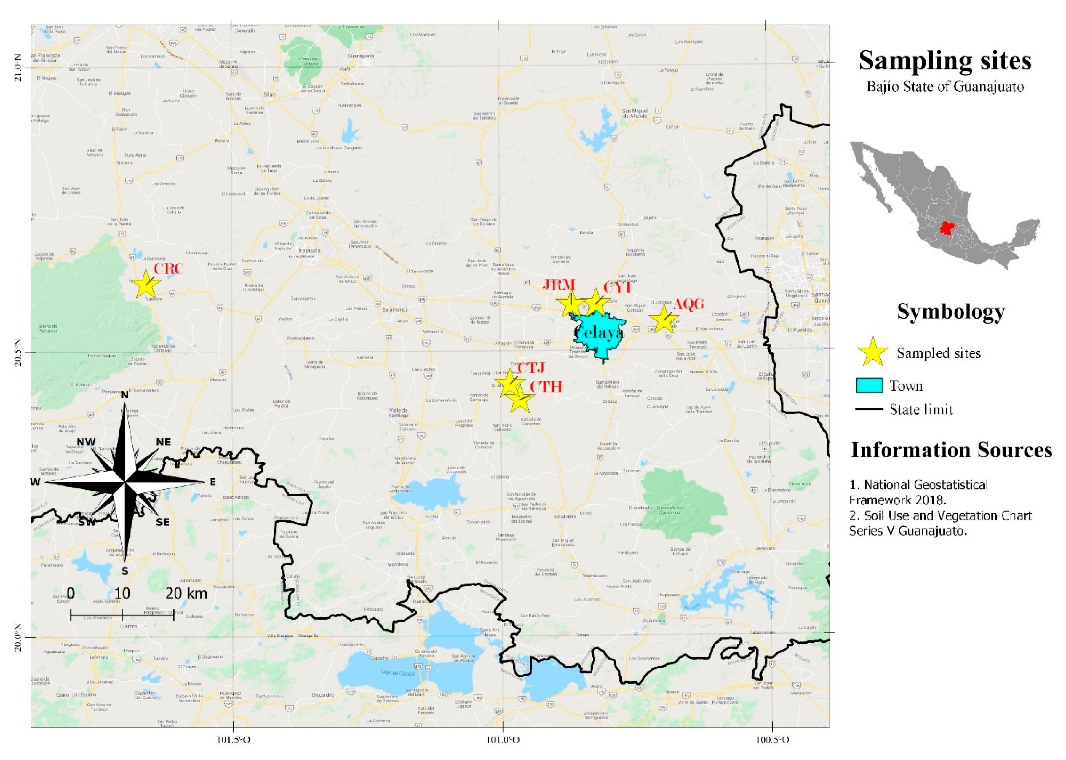
2.1. Survey and Sampling Soils

This study was carried out in the lowland plains region of the state of Guanajuato, which altitude ranges from 1700 to 1800 m.a.s.l. The predominant soils are those of the Chernozem type, with an annual rainfall of 700 mm and an average annual temperature between 18 and 22 °C [14]. Six agricultural soils were selected from the region because of their agricultural management history (

Table 1. Agricultural management of sampled soils from Guanajuato’s lowlands.

Agricultural Management	Soils
	AGQ	CTH	CTJ	JRM	CRC	CYI
Crop	Fodder corn/triticale forage	Alfalfa	Sorghum/barley	No cultivation, only natural grass	Corn/barley	Bean
Soil management	gypsum/compost (cow dung)	-	-	-	-	-
Type of irrigation	Surface with well water	Surface with well water	Surface with well water	Seasonal	Surface with well water/thermal water	Surface with well water
Fertilization practices	Treatment 240–60–0 kg/ha for corn	100 kg of sulphates/ha	Treatment 300–60–0 kg/ha for sorghum/200–60–0 kg/ha for barley	None	Treatment 200–60–0 kg/ha for barley/240–60–0 kg/ha for corn	Treatment 80–40–0 kg/ha for beans
Tillage	Conventional (1 fallow, 4 harrows, 1 crop)	Only soil preparation when the crop was established, then zero tillage.	Conventional (1 fallow, 4 harrows, 1 crop)	Zero tillage because it is not sowed or cultivated, only the grass is used in temporary conditions	Conventional (1 fallow, 4 harrows, 1 crop)	Conventional with only one cycle per year (1 fallow, 2 harrows, 1 crop)
Yield	80 t of silo/ha	350 bales/ha	8 t sorghum/ha 4.5 t barley/ha	Not estimated	10 t maize/ha 6 t barley/ha	2 t beans/ha
Location	20°33′4.72″ N, 100°41′40.11″ W	20°24′50.22″ N, 100°57′50.84″ W	20°26′28.32″ N, 100°58′57. 50″ W	20°34′50.44″ N, 100°51′59.78″ W	20°37′82″ N, 101°39′35.86″ W	20°34′52.77″ N, 100°49′16.41″ W

AGQ = Apaseo El Grande, CTH = Cortazar El Huizache, CTJ = Cortazar Rancho El Jore, JRM = Santa Cruz Juventino Rosas Merino, CRC = Cuerámaro Rancho Cuarto Blanco, CYI = INIFAP Celaya Parcel 12, t = metric tons, ha = hectare. Fertilization practices are based on established NPK units, using urea-based fertilizers and triple calcium superphosphate.

). In the experimental field of Celaya, Guanajuato, the National Institute of Forestry, Agricultural and Livestock Research (INIFAP) had previously identified these soils with a tendency to have problematic rates of alkalinity, salinity, and sodicity.

The analyzed soils (Figure 1) were located in Apaseo El Grande “AGQ” (20°33′4.72″ N, 100°41′40.11″ W), Cortazar El Huizache “CTH” (20°24′50.22″ N, 100°57′50.84″ W), Cortazar Rancho El Jore “CTJ” (20°26′28.32″ N, 100°58′57.50″ W), Santa Cruz Juventino Rosas Merino “JRM” (20°34′50.44″ N, 100°51′59.78″ W), Cuerámaro Rancho Cuarto Blanco “CRC” (20°37′82″ N, 101°39′35.86″ W), and INIFAP Celaya “CYI”, Parcel 12 (20°34′52.77″ N, 100°49′16.41″ W).

The sampling consisted of dividing each plot into three sub-plots of 600 m² each. The sampling was systematic and random, starting at one end of each subplot and moving forward in a zigzag pattern [15]. The subsamples were taken every 18 m, using an auger with which wells of 40 cm in diameter and 30 cm in depth were made, taking approximately 2 kg of soil for each subsample. Fifteen subsamples were obtained from each subplot, which meant a total of 45 subsamples per sampled soil; with a total of 270 samples for the six soils analyzed After selection, the total weight of each sample was 10 kg. Each sampled soil was georeferenced using a Garmin^® eTrex Legend^® H GPS receiver.

2.2. Preparation and Maintenance of Soil Samples

To perform the biological analyses, the soil samples were taken to the laboratory in sterile plastic bags and were refrigerated at 4 °C until their respective analyses [16,17,18]. For the physicochemical analyses, subsamples of the soils were mixed and transported at room temperature to the laboratory. Then, the subsamples were air-dried and screened with a clean mesh with an opening diameter of 2 mm. Once dried and sieved, they were stored in plastic bags at 4 °C for further physicochemical analysis [16,17,18].

2.3. Sample Preparation for the Establishment of Physicochemical Indicators

The physicochemical indicators related to soil fertility were determined in triplicate. The texture was determined by granulometric analysis, using the hydrometer method established by Bouyoucos [19], reporting percentage of sand, silt, and clay. The texture diagram proposed by the USDA was used to establish the textural class [20]. The potential of hydrogen (pH) was determined by Thomas’s method [21], using a soil:water ratio of 1:2.5 (w/v). The electrical conductivity (EC) was determined by the method of Hendrickx et al. [22], reporting in dS m⁻¹. The pH and EC were determined using a Horiba Scientific F-74BW potentiometer and EC meter. The water content was determined by weight difference and reported in % of humidity, using 20 g of soil and drying at 105 °C (±2) for 24 h in a Riossa H-33 stove [23]. The water holding capacity (WHC) was determined using the methodology described by Nannipieri [23], i.e., by placing 20 g of soil on a Whatman No. 2 filter paper, adding 100 mL of distilled water, and leaving it to stand for 24 h. The WHC was calculated by the difference in weight between the value obtained and the weight of the filter without soil (“soilless target”), reported as % of WHC. The bulk density (BD) was determined by the method established by Blake and Hartage [24], reported in g mL⁻¹. Total organic carbon (TOC) was established according to the method of Walkley and Black [25], i.e., by chemical digestion with potassium dichromate and quantified colorimetrically at 600 nm in a Jenway 6305 spectrophotometer, reported in g C per kg dry soil. The percentage of organic matter (OM) was obtained with the TOC value and multiplied by the Van Bemmelen factor (1.724) [15,26]. The total nitrogen (TN) was determined using the micro Kjeldahl method [27], quantified colorimetrically at 660 nm using a spectrophotometer as described above, reported in mg N per kg of dry soil. Inorganic nitrogen—expressed as ammonium (N-NH₄⁺), nitrites (N-NO₂⁻), and nitrates (N-NO₃⁻)—was analyzed by prior extraction with K₂SO₄ (0.5 M of potassium sulfate), at a ratio w/v of 1:5 for 2 h [28]. After extraction, the extract was filtered with a Whatman No. 2 filter paper. To analyze ammonium-nitrogen (N-NH₄⁺), a solution of salicylic acid (5% w/v) was used, and colorimetric determinations were performed at a wavelength of 660 nm [23]. A solution of diazonium salt (0.3% w/v) was used for the analysis of nitrites (N-NO₂⁻), and colorimetric determinations were performed at a wavelength of 410 nm [23]. For the analysis of nitrates (N-NO₃⁻), a sulfanilamide solution (0.5% w/v) was used, and colorimetric determinations were performed at a wavelength of 540 nm [23]. The forms of inorganic nitrogen were reported as mg N-NH₄⁺ per kg dry soil, mg N-NO₂⁻ per kg dry soil, and mg N-NO₃⁻ per kg dry soil. Potassium (K⁺), calcium (Ca⁺²), magnesium (Mg⁺²), and sodium (Na⁺) ions were quantified using the microwave digestion/ICP [29], reported in meq. per 100 g of dry soil. The cation exchange capacity (CEC) was obtained following the methodology described by Cottenie [30], reported in meq. per 100 g of dry soil. Exchangeable sodium percentage (ESP) and sodium adsorption ratio (SAR) were estimated following the methodology described by SEMARNAT [15] and Hazelton and Murphy [31], reported in percentage.

2.4. Biological Characterization

Indicators related to the microbial biomass and its enzymatic activity were analyzed in order to establish the biological indicators. The carbon of the microbial biomass (MBC) was determined by the substrate-induced respiration (SIR) method, which is based on the addition of an assimilable substrate (glucose) with the subsequent capture and quantification of the C-CO₂ emitted by the microbial biomass under aerobic conditions and captured in an alkaline medium of NaOH 1.0 M. The captured C-CO₂ was reported in mg C_mic kg dry soil⁻¹ [32]. The metabolic quotient (qCO₂)—related to cell respiration and used as a measure of the ecophysiological status of microorganisms in the soil [8,33], was estimated in terms of the emission of g C-CO₂ per kg of dry soil under aerobic incubation conditions at room temperature for 10 h [34]. The emitted C-CO₂ was captured with 1.0 M NaOH solution and calculated by titration with 0.1 M HCl [28]. The calculated C-CO₂ was divided by MBC unit and expressed as g C-CO₂ mg C_mic⁻¹ h⁻¹ [34]. The microbial quotient (qMic) was measured as well, which establishes the availability and carbon conversion efficiency of organic matter (OM) present in MBC. In addition, the qMic has also been used to estimate the microbial activity and the accumulation of OM in the soil, estimated as a ratio MBC:TOC, reported in % [35,36]. With regard to the use of biological indicators sensitive to change or disturbance in agricultural soils [16,37,38,39,40,41,42], enzymatic activities were analyzed, mainly the ones related to the metabolic status of microbial biomass and enzymatic activities and the ones related to fertility and C, N, and P cycles. The enzymatic activity of dehydrogenase (DHA) was quantified by colorimetric detection of formazan (INF) after an incubation period of 2 h at 40 °C and 464 nm wavelength, reported in µg INF kg of dry soil⁻¹ h⁻¹ [43]. Urease activity (UA) was determined after an incubation period of 2 h at 37 °C, based on the colorimetric determination of ammonium released at 640 nm wavelength and reported in µg N-NH₄⁺ kg dry soil⁻¹ h⁻¹ [44]. The overall enzymatic activity of proteases, lipases, and esterases were determined by the hydrolysis of fluorescein diacetate (FDA). The FDA activity was quantified by a colorimetric method based on the detection of fluorescein after an incubation period of 1 h at 35 °C and detected at 490 nm, reported in µg of fluorescein kg of dry soil⁻¹ h⁻¹ [45]. Moreover, a Shannon microbial diversity index (H’) was included as one of the biological indicators used for the establishment of the SQI. The H’ index evaluates the diversity of enzymatic functions, where higher values of the indicator reflect that the microorganisms in the soil have a greater metabolic capacity [46].

Equation (1) was used to establish the Shannon index (H’), using the concentration of enzymatic activities included in the bioMérieux^® semi-quantitative system known as API ZYM^®. The results of the enzymatic hydrolytic activities of the API ZYM^® system are determined after an incubation period of 4 h at a temperature of 37 °C. The reactions of enzymatic activity generate color patterns, which are compared with a color code and established intensities: very high-intensity level 5 (40 nmol), high-intensity level 4 (30 nmol), medium-intensity level 3 (20 nmol), low-intensity level 2 (10 nmol), very low-intensity level 1 (5 nmol), and no intensity level 0 (0 nmol) [41,42,46,47,48]. The API ZYM^® system includes the following enzyme activities: alkaline phosphomonoesterase (AP), acid phosphomonoesterase (APE), phosphohydrolase (PH), esterase (ES), esterase lipase (EL), lipase (LIP), leucine arylamidase (LAA), valine arylamidase (VAA), cystine arylamidase (CAR), trypsin (TRI), α-chymotrypsin (AC), α-galactosidase (AGAL), β-galactosidase (BGAL), β-glucuronidase (BGLU), α-glucosidase (AGLU), β-glucosidase (BGLUC), N-acetyl-β-glucosaminidase (NABG), α-mannosidase (AMAN) and α-fucosidase (AFUC) [46,49].

Likewise, another enzyme index was developed, which is called the “synthetic enzyme index” (SEI). This index reflects the total enzymatic diversity, related to the fertility and biogeochemical cycles of C, N, and P. In previous studies reported in the literature, this index has been developed from the API ZYM^® system in various types of soils [46]. However, the SEI index developed in this study—in addition to using the concentrations of enzyme activities from the API ZYM^® system—included the enzyme activities of dehydrogenase (DHA), urease (UA), and fluorescein diacetate (FDA) (Equation (2)). The API ZYM^® system has proven to be a fast and useful tool in establishing profiles of point or space-time “fingerprint” enzymatic activities in complex environmental matrices, such as soils, compost, vermicompost, activated sludge, biosolids, and sediments [41,42,46,48,50,51,52].

$${\mathrm{H}}^{\prime }=-{{\displaystyle \sum }}_{i=1}^k\left(X_i\ast \ln \left(X_i\right)\right)$$

(1)

and

$$SEI={{\displaystyle \sum }}_{i=1}^k{X}_i$$

(2)

where $X_i$ for Equation (1) is the ratio of the enzyme activity to the total enzyme activity, while for Equation (2) is the intensity of the enzyme activity obtained from the API ZYM^® system and the enzyme activities DHA, UA, and FDA, respectively.

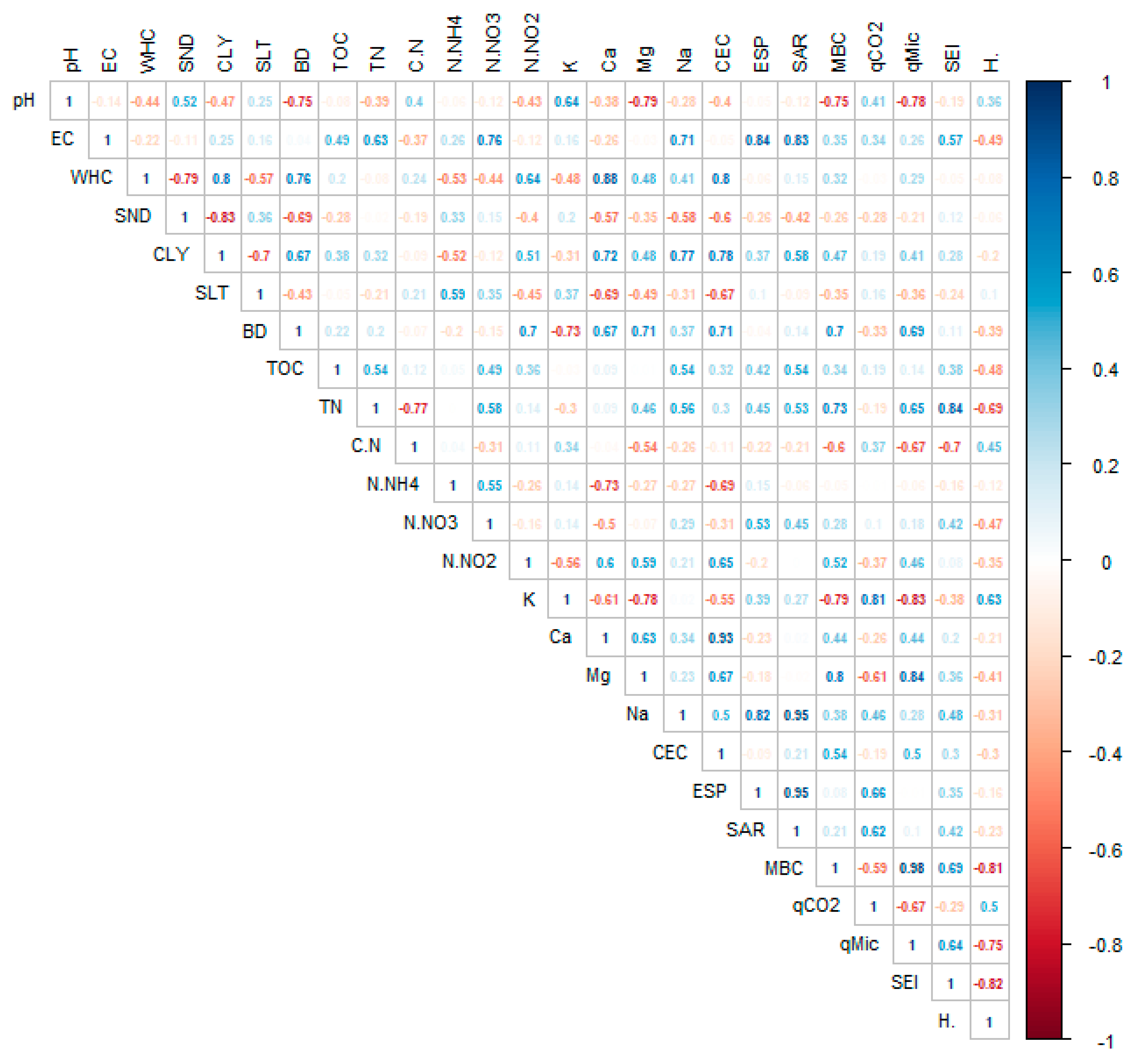
2.5. Statistical Analysis

The statistical analysis was carried out using the R Statistical Software version 3.6.3 [53]. The differences between the indicators were measured using a one-way analysis of variance (ANOVA) and a subsequent analysis of Tukey means and Fisher value with a significance level $p \le 0.05$. Correlations were established among the indicators analyzed by means of a Pearson’s product-moment correlation matrix, those indicators with an $r^2\ge 0.6$ [16]. For the principal component analysis (PCA), indicator data were normalized using natural logarithms, followed by a Kaiser–Meyer–Olkin adequacy analysis [54,55], whose purpose is to observe the feasibility of using the data for the PCA [56]. Once the principal components (PCs) were obtained, the eigenvalue selection criterion was used, which represents the variance of each one of the PCs, selecting those with an eigenvalue > 1 [56,57]. Once the PCs with an eigenvalue greater than 1 were established, the indicators that had a significant linear correlation with their principal component (PC) were selected $r^2\ge 0.6$ [17,18], with a commonality with the PC ≥ 0.6, which represents the proportion of the variation of the respective component. Subsequently, a process of redundancy reduction was carried out among the indicators, which results are significantly related to their respective PC, and appear under the following criteria and in order of importance: the number of significant interactions with other indicators > PC belonging (PC1 > PC2 > PC3 > ... > PCn) > correlation with its PC. To establish the SQI, the resulting indicators and their correlations were standardized to a range of 0 to 1 [17].

2.6. Development of the SQI

The SQI was established following the methodologies employed by Yu et al. [57], using an additive weighting Equation (3) and an indicator scoring Equation (4) [57]. The equation of additive weights was used, using the PC variability obtained from the SQI development process, giving a greater precision in establishing the quality of the soils. This gives advantages over other techniques (equation of fixed additive weights, experts’ opinion, and linear additive indexes); being one of the techniques with greater adoption by the community, allowing its comparison with other studies.

$$SQI{ }_W={{\displaystyle \sum }}_{i =1}^n{W}_i{S}_i$$

(3)

where: $W_i$ is the proportion of variability of the PC to which the indicator is correlated, $S_i$ is the value of the indicator resulting from the redundancy reduction process, obtained from the analysis of the soil samples. Equation (4) was used to score indicators whose function in the soil is “the more the better,” or “the less the better”:

$$S_i=\frac{a}{1+{\left(\frac{X}{X_m}\right)}^b}$$

(4)

where: $a$ is equal to the maximum standardized value of the indicator, $X_m$ is the average value of the indicator obtained from the analyses, $X$ is the value of the indicator and $b$ is the slope of the indicator’s scoring function (−2.5 for indicators whose function is “the more the better” and 2.5 for indicators whose function is “the less the better”).

Equation (5), was used to score indicators whose function in the soil is considered “optimal” and whose maximum or optimal value is at the value of 0.5 [58]:

$$S_i=\frac{1}{\left[1+{\left(\frac{\left(B-L\right)}{\left(X-L\right)}\right)}^{2L\left(B+X-2L\right)}\right]}$$

(5)

where: $B$ is the indicator value where the slope is equal to 0.5, $L$ is the lowest limit value of the indicator and $X$ is the indicator value. The objective of the SQI was to establish a value between 0 and 1, thus establishing the soil quality according to the classification shown in

Table 2. Soil quality classification [59].

Soil Quality	Very High	High	Moderate	Low	Very Low
Scale	0.80–1.00	0.60–0.79	0.40–0.59	0.20–0.39	0.00–0.19
Class	1	2	3	4	5

.

3. Results

3.1. Physicochemical Indicators

The values of the physicochemical indicators are shown below (

Table 3. Values of physicochemical indicators of analyzed soils from Guanajuato’s lowlands.

DV	Soils
	AGQ	CTH	CTJ	JRM	CRC	CYI
pH	8.40 ± 0.15	8.07 ± 0.14	7.82 ± 0.11	8.85 ± 0.22	7.80 ± 0.18	8.57 ± 0.10
EC	0.87 ± 0.11	0.81 ± 0.04	0.71 ± 0.05	1.22 ± 0.12	1.78 ± 0.27	0.61 ± 0.12
WHC	94.83 ± 4.61	180.55 ± 16.98	167.45 ± 6.33	116.37 ± 5.45	101.79 ± 8.08	91.93 ± 5.67
SND	34.63 ± 4.62	14.75 ± 4.07	9.10 ± 3.59	17.19 ± 2.25	18.03 ± 3.18	34.82 ± 4.89
CLY	40.24 ± 3.81	62.93 ± 3.99	69.18 ± 7.29	52.27 ± 6.24	48.94 ± 3.19	26.18 ± 3.68
SLT	25.13 ± 4.28	22.32 ± 4.76	21.72 ± 5.59	30.55 ± 7.75	33.03 ± 2.81	39.00 ± 4.95
BD	0.94 ± 0.03	1.13 ± 0.01	1.10 ± 0.002	0.94 ± 0.03	1.06 ± 0.02	0.94 ± 0.01
TOC	10.97 ± 2.27	13.12 ± 1.17	11.02 ± 0.46	13.53 ± 0.82	14.06 ± 0.95	10.30 ±1.98
TN	468.71 ± 56.34	391.22 ± 26.41	336.77 ± 28.49	351.28 ± 38.58	552.50 ± 36.11	252.00 ± 29.99
C/N	23.28 ± 2.72	33.63 ± 3.23	32.84 ± 1.70	38.88 ± 4.10	25.59 ± 2.81	40.79 ± 4.91
N-NH4+	24.70 ± 4.21	23.23 ± 3.62	25.91 ± 7.57	29.89 ± 6.05	63.63 ± 14.51	56.23 ± 10.87
N-NO2−	0.62 ± 0.19	1.13 ± 0.30	0.88 ± 0.16	0.59 ± 0.12	0.73 ± 0.05	0.63 ± 0.12
N-NO3−	23.78 ± 7.50	18.46 ± 3.01	15.56 ± 3.39	25.52 ± 1.51	55.32 ± 7.25	21.27 ± 3.30
K+	1.85 ± 0.15	0.87 ± 0.10	1.79 ± 0.15	4.57 ± 0.54	1.66 ± 0.27	2.42 ± 0.20
Ca+2	24.95 ± 1.94	48.87 ± 1.80	34.94 ± 1.58	20.59 ± 1.36	17.62 ± 1.67	15.27 ± 0.59
Mg+2	8.20 ± 0.60	10.05 ± 1.92	10.79 ± 1.33	3.31 ± 0.13	8.47 ± 0.63	4.43 ± 0.43
Na+	2.79 ± 0.15	4.00 ± 0.18	4.30 ± 0.43	6.07 ± 0.74	5.56 ± 1.03	1.09 ± 0.27
CEC	37.70 ± 4.50	63.55 ± 5.00	52.80 ± 10.63	34.50 ± 3.63	33.33 ± 2.64	23.20 ± 2.88
ESP	7.44 ± 0.57	6.31 ± 0.38	8.42 ± 1.90	17.78 ± 3.17	16.81 ± 3.44	4.76 ± 1.34
SAR	2.16 ± 0.04	2.33 ± 0.11	2.81 ± 0.26	5.54 ± 0.52	4.88 ± 0.94	1.09 ± 0.24

DV = dependent variable, pH = potential of hydrogen, EC = electrical conductivity (dS m⁻¹), WHC = water holding capacity (%), SND = sand (%), CLY = clay (%), SLT = silt (%), BD = bulk density (g mL⁻¹), TOC = total organic carbon (g C kg dry soil⁻¹), TN = total nitrogen (mg N kg dry soil⁻¹), C/N = carbon to nitrogen ratio, N-NH₄⁺ = ammonium (mg N-NH₄⁺ kg dry soil⁻¹), N-NO₂⁻ = nitrites (mg N-NO₂⁻ kg dry soil⁻¹), N-NO₃⁻ = nitrates (mg N-NO₃⁻ kg dry soil⁻¹), K⁺ = potassium (meq. 100 g⁻¹), Ca⁺² = calcium (meq. 100 g⁻¹), Mg⁺² = magnesium (meq. 100 g⁻¹), Na⁺ = sodium (meq. 100 g⁻¹), CEC = cation exchange capacity (meq. 100 g⁻¹), ESP = exchangeable sodium percentage (%), SAR = sodium adsorption ratio (%). The values are the average of the results per indicator ± the standard deviation (12 repetitions).

). The soils analyzed presented a pH between 7.80 and 8.85, establishing three categories, slightly alkaline (CRC), moderately alkaline (CTJ and CTH), and strongly alkaline (AGQ, CYI, and JRM) [15,31]. Concerning the EC indicator, the soils were found in the interval of 0.61 to 1.78 dS m⁻¹, all of them considered as non-saline [15,31]. The WHC indicator was found in a range of 91.93 to 180.55%, establishing two categories, low capacity (CYI and AGQ), and moderate capacity for the remaining soils [29]. The texture test showed clayey soils (CTH, CTJ, JRM, and CRC), and clay loam soils (AGQ and CYI) [20]. The soils presented BD values between 0.94 and 1.12 g mL⁻¹, establishing two categories, very low density (AGQ and JRM), and low density for the remaining soils [31].

The TOC values ranged from 10.31 to 14.06 g C kg dry soil⁻¹, which is considered to be low for all of the analyzed soils [15,31]. The C/N ratio showed values between 23.28 and 40.79, establishing two categories, medium ratio (AGQ), and high ratio for the remaining soils [31]. According to the TN indicator, the soils showed values that range from 252.0 to 552.5 mg N kg dry soil⁻¹, which is considered to be very low for all of the analyzed soils [15,31]. Regarding the indicator N-NH₄⁺, the soils presented values that range from 23.23 to 63.63 mg N-NH₄⁺ kg dry soil⁻¹, and for the indicator N-NO₂⁻ the values ranged from 0.59 to 1.13 mg N-NO₂⁻ kg dry soil⁻¹. The indicator N-NO₃⁻ presented values in the range of 15.56 and 55.32 mg N-NO₃⁻ kg dry soil⁻¹ [15,31].

With regard to the cations that were analyzed, K⁺ presented values in the range of 0.87 to 4.57 meq. 100 g⁻¹, establishing two categories, high concentration (CTH, CRC, CTJ, and AGQ), and very high (CYI and JRM) [15,31]. In reference to the Ca⁺² cation, the soils showed values in the interval of 15.27 to 48.87 meq. 100 g⁻¹, establishing two categories, high concentration (CYI and CRC), and very high (JRM, AGQ, CTJ, and CTH) [15,31]. The Mg⁺² cation showed values in the range of 3.31 to 10.79 meq. 100 g⁻¹, establishing two categories, high concentration (JRM and CYI), and very high (AGQ, CRC, CTH, and CTJ) [15,31]. The Na⁺ cation had values in the interval of 1.09 to 6.07 meq. 100 g⁻¹, considered to be high for the CYI soil and very high for the other soils [15,31]. In relation to the CEC indicator, the soils presented values in the interval of 23.20 to 63.70 meq. 100 g⁻¹, establishing three categories, moderate concentration (CYI), high concentration (CRC, JRM, and AGQ), and very high concentration (CTJ and CTH) [31]. The soils presented ESP values in the interval of 4.64 to 17.52%, establishing three categories, non-sodic (CYI), marginally sodic (CTH, AGQ, and CTJ), and strongly sodic (CRC and JRM) [31]. The sodium adsorption ratio (SAR) showed values in the range of 0.66 to 3.27%, indicating the concentration of Na⁺ cation with respect to Ca⁺² and Mg⁺² cations in the soil solution. The ESP indicator showed a similar interaction of the Na⁺ cation with the other divalent cations in the soil exchange complex [31].

3.2. Ecophysiological Indicators

The MBC indicator—related to the quantity of microorganisms present in the soil—showed values in the range of 166.59 to 1222.80 mg C_mic kg dry soil⁻¹ (

Table 4. Values of ecophysiological indicators of analyzed soils from Guanajuato’s lowland.

DV	Soils
	AGQ	CTH	CTJ	JRM	CRC	CYI
MBC	536.57 ± 100.58	1014.95 ± 109.00	460.74 ± 60.39	166.59 ± 26.37	1222.84 ± 36.91	171.65 ± 32.32
qCO2	3.25 ± 1.04	2.54 ± 0.41	8.02 ± 1.37	33.07 ± 5.27	5.18 ± 0.12	4.31 ± 1.01
qMic	0.05 ± 0.01	0.08 ± 0.00	0.04 ± 0.00	0.01 ± 0.00	0.09 ± 0.01	0.02 ± 0.01

DV = dependent variable, MBC = microbial biomass carbon (mg C_mic kg dry soil⁻¹), qCO₂ = metabolic quotient (g C-CO₂ mg C_mic⁻¹ h⁻¹), qMic = microbial quotient (ratio of microbial carbon to total organic carbon MBC/TOC). The values are the mean of the results per indicator ± the standard deviation (12 repetitions).

), being the JRM soil the one with the lowest value, while the CRC soil presented the highest value. The indicator qCO₂—which has been used to measure the microbial population disturbance due to agricultural soil management conditions—presented values in the range of 2.54 to 33.07 g C-CO₂ mg C_mic⁻¹ h⁻¹ (Table 4). The CTH and JRM soils presented the highest and lowest value of qCO₂, respectively. The qMic indicator—which reflects the amount of OM that is usable by the microbial community in soils; presented values in the interval of 0.01 to 0.09% (Table 4), with the CYI and JRM soils having the lowest percentage, and the CRC soil having the highest percentage.

3.3. Enzyme Profile

In reference to enzyme analyses obtained from the API ZYM^® enzyme system and direct enzyme activity analyses (UA, DHA, and FDA) (

Table 5. Enzymatic activities in the sampled soils from Guanajuato’s lowlands.

Enzyme (µmol of Substrate kg of Soil−1)	Soils
	AGQ	CTH	CTJ	JRM	CRC	CYI
UA	41,813.39	2429.36	766.71	7135.49	32,733.67	680.78
DHA	1.72	2.87	11.83	6.94	21.40	7.51
FDA	168.19	3054.26	131.72	136.65	58.74	59.16
AP	0.010	0.040	0.040	0.020	0.040	0.005
APE	0.010	0.010	0.030	0.005	0.030	0.005
PH	0.020	0.030	0.020	0.020	0.020	0.020
ES	---	---	---	---	---	---
EL	0.010	0.030	0.020	0.020	0.030	0.010
LIP	0.020	0.020	0.010	0.010	0.020	0.010
LAA	0.005	0.005	0.005	0.005	---	0.005
VAA	---	---	---	---	---	---
CAR	0.020	0.020	0.030	0.020	0.010	0.010
TRI	0.020	0.010	0.020	0.020	0.010	0.010
AC	0.005	0.005	0.010	0.010	0.020	0.005
AGAL	---	---	---	---	---	---
BGAL	0.005	---	0.010	0.005	0.005	---
BGLU	---	---	---	---	---	---
AGLU	0.005	0.005	0.005	0.005	0.005	---
BGLUC	---	---	---	---	---	---
NABG	0.005	0.005	---	---	---	---
AMAN	0.005	0.005	0.005	---	---	---
AFUC	---	---	---	---	---	---

UA = urease activity, DHA = dehydrogenase activity, FDA = fluorescein diacetate activity, AP = alkaline phosphomonoesterase, APE = acid phosphomonoesterase, PH = phosphohydrolase, ES = esterase, EL = esterase lipase, LIP = lipase, LAA = leucine arylamidase, VAA = valine arylamidase, CAR = cystine arylamidase, TRI = trypsin, AC = α-chymotrypsin, AGAL = α-galactosidase, BGAL = β-galactosidase, BGLU = β-glucuronidase, AGLU = α-glucosidase, BGLUC = β-glucosidase, NABG = N-acetyl-β-glucosaminidase, AMAN = α-mannosidase, AFUC = α-fucosidase.

and

Table 6. Enzymatic profile by families (API ZYM^® system) of sampled soils from Guanajuato’s lowlands.

Families	Enzymes	Soils
		AGQ	CTH	CTJ	JRM	CRC	CYI
Phosphatases	AP
	APE
	PH
Esterases-lipases	ES
	EL
	LIP
Aminopeptidases	LAA
	VAA
	CAR
Peptidases	TRI
	AC
Glycosyl hydrolases	AGAL
	BGAL
	BGLU
	AGLU
	BGLUC
	NABG
	AMAN
	AFUC
	Activity $\ge$ 1	13	12	12	11	10	9
	Activity $\ge$ 2	7	4	5	7	5	5
	Activity $\ge$ 4	0	3	4	0	3	0
	Not detected	6	7	7	8	9	10

= high intensity 30 to 40 nmol kg of dry soil⁻¹, = medium intensity 10 to 20 nmol kg of dry soil⁻¹, = low intensity 5 nmol kg of dry soil⁻¹ and = not detected.

), a variation in enzyme activities was observed with respect to the sampled soils. The overall enzyme activities presented a sequence from highest to lowest in the following order: CTJ > CRC > CTH > AGQ > JRM > CYI. With regard to the individual enzyme activities, the following order was established from highest to lowest: EL > PH, CAR > AP, LIP = TRI > APE > AC > BGAL > LAA = AGLU > AMAN > NABG. The enzymes ES, VAA, AGAL, BGLU, BGLUC, and AFUC were not detected in the analyzed soils (Table 6). Differences in enzymatic activities at family level were observed, obtaining activities in the following order from highest to lowest: phosphatases > esterase lipase > peptidases > aminopeptidases > glycosyl hydrolases (Table 6).

In the SEI indicator, soils showed values in the range of 747.79 to 41,983.45 µmol kg dry soil⁻¹ with the CYI soil showing the lowest enzymatic activity and the AGQ soil showing the highest activity. Finally, in the indicator H’, soils showed values in the interval of 2.35 to 3.08 (

Table 7. Values of the synthetic enzyme index (SEI) and enzyme functional diversity indicator (H’) in the analyzed soils of Guanajuato’s lowlands.

DV	Soils
	AGQ	CTH	CTJ	JRM	CRC	CYI
SEI	41,983.45 ± 4848.38	24,290.04 ± 1433.42	910.53 ± 175.61	7279.12 ± 2501.91	32,814.06 ± 3287.31	747.79 ± 66.82
H’	2.65 ± 0.04	2.35 ± 0.02	3.08 ± 0.08	2.91 ± 0.10	2.35 ± 0.03	2.97 ± 0.03

DV = dependent variable, SEI = synthetic enzyme index (µmol kg dry soil⁻¹), H’ = Shannon diversity index. The values are the mean of the results per indicator ± the standard deviation (12 repetitions).

), which is considered to be a moderate functional enzymatic diversity for all tested soils.

Table 7 shows the values of the biochemical indicators H’ and SEI, obtained from the data in Table 5. In the analyzed soils, the SEI indicator presented the following order of activity from highest to lowest: AGQ > CRC > CTH > JRM >CTJ > CYI. With respect to the indicator H’, the microbial diversity—from highest to lowest—is presented as follows: CTJ > CYI > JRM > AGQ > CRC = CTH.

3.4. Analysis of Variance

The ANOVA test (

Table 8. One-way ANOVA (with Tukey test) of soil indicators analyzed from Guanajuato’s lowlands.

DV	Soils						F	p
	AGQ	CTH	CTJ	JRM	CRC	CYI
pH **	8.40b	8.07c	7.82d	8.85a	7.80d	8.57b	90.39	0.000
EC **	0.87c	0.81c	0.71cd	1.22b	1.78a	0.61d	117.24	0.000
WHC **	94.83d	180.55a	167.45b	116.37c	101.79d	91.93d	226.54	0.000
SND **	34.63a	14.75b	9.10c	17.19b	18.04b	34.82a	92.86	0.000
CLY **	40.24d	62.93b	69.18a	52.27c	48.94c	26.18e	118.58	0.000
SLT **	25.13cd	22.32d	21.72d	30.55bc	33.03ab	39.00a	20.15	0.000
BD **	0.94d	1.12a	1.10b	0.94d	1.06c	0.94d	199.57	0.000
TOC **	10.97b	13.13a	11.02b	13.53a	14.06a	10.31b	14.78	0.000
TN **	468.70b	391.22c	336.77d	351.30cd	552.50a	252.00e	96.20	0.000
C/N **	23.28c	33.63b	32.85b	38.88a	25.59c	40.79a	50.44	0.000
N-NH4+ **	24.70b	23.23b	25.91b	29.89b	63.63a	56.23a	50.57	0.000
N-NO2− **	0.62c	1.13a	0.89b	0.59c	0.73bc	0.63c	17.31	0.000
N-NO3− **	23.78bc	18.46cd	15.56d	25.53b	55.32a	21.27bcd	106.14	0.000
K+ **	1.85c	0.87d	1.79c	4.57a	1.66c	2.42b	250.08	0.000
Ca+2 **	24.95c	48.87a	35.94b	20.59d	17.62e	15.27f	823.55	0.000
Mg+2 **	8.20b	10.05a	10.79a	3.31c	8.47b	4.43c	102.75	0.000
Na+ **	2.79c	4.00b	4.30b	6.07a	5.56a	1.09d	125.91	0.000
CEC **	37.78c	63.70a	52.82b	34.54c	33.32c	23.20d	508.85	0.000
ESP **	7.39bc	6.27c	8.14b	17.52a	16.67a	4.64d	211.09	0.000
SAR **	1.30c	1.38bc	1.69b	3.27a	3.00a	0.66d	151.71	0.000
MBC **	536.60c	1014.90b	460.70c	166.59d	1222.80a	171.65d	478.24	0.000
qCO2 **	3.25c	2.54c	8.02b	33.07a	5.18c	4.31c	311.28	0.000
qMic **	0.05c	0.08b	0.04d	0.01e	0.09a	0.01e	293.73	0.000
SEI **	41,983.0a	24,290.0c	910.5e	7279.0d	32,814.0b	747.8e	519.41	0.000
H’ **	2.65c	3.08a	2.35d	2.91b	2.35d	2.97b	367.72	0.000

DV = dependent variable, F = Fisher value, p = probability value. Values in bold indicate the maximum and minimum data for each indicator, same letters in the rows indicate that there is no significant difference among the soils sampled using the one-way ANOVA test, with subsequent Tukey test. (**) Means that the test was statistically significant for the indicator under $p \le 0.05$ and $p \le 0.01$, respectively.

) showed that the analyzed indicators presented significant differences ($p \le 0.05$) among the analyzed soils and a high correlation ($r^2\ge 0.6$) with the one-way ANOVA model, except for the TOC and N-NO₂⁻ indicators, whose correlation was low ($r^2< 0.6$). However, the results of Fisher values and probability were significant ($F \ge 5.0$ and $p \le 0.5$) for all of the indicators, and Fisher values of 14.78 and 17.31 were obtained for the TOC and N-NO₂⁻ indicators, respectively. The results obtained made it possible to analyze the indicators individually and to establish which of them presented differences in the analyzed soils, which allowed for the subsequent establishment of the SQI.

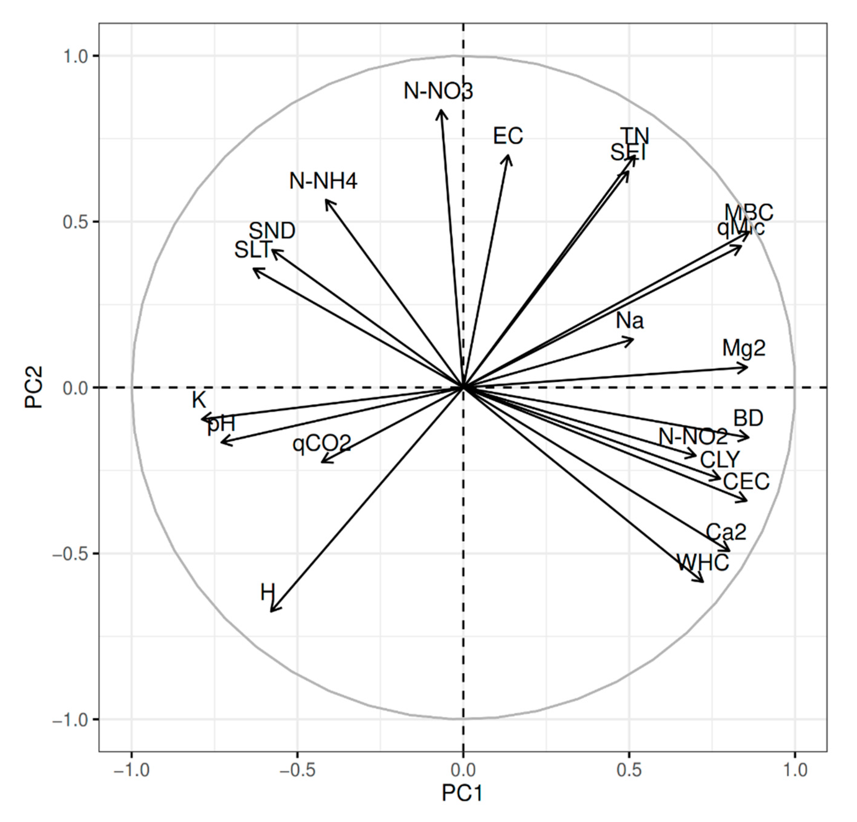
3.5. Principal Component Analysis

The analysis of Pearson’s product-moment correlation coefficient (Figure 2) showed that all of the indicators presented a significant correlation ($r^2\ge \pm 0.6$), except for the TOC indicator which showed no correlation with any other indicator.

Table 9. Significant correlations among the various indicators.

Indicator	Significant Positive Correlation with Other Indicators	Significant Negative Correlation with Other Indicators
pH	K+	BD, Mg+2, MBC, and qMic
EC	TN, N-NO3−, Na+, ESP, and SAR	---
WHC	CLY, BD, N-NO2−, Ca+2, and CEC	SND
SND	---	WHC, CLY, BD, and CEC
CLY	WHC, BD, Ca+2, Na+, and CEC	SND and SLT
SLT	---	SND, Ca+2, and CEC
BD	WHC, CLY, N-NO2−, Ca+2, Mg+2, CEC, MBC, and qMic	pH, SND, and K+
TOC	---	---
TN	EC, MBC, qMic, and SEI	C/N and H’
N-NH4+	---	Ca+2 and CEC
N-NO3−	EC	---
N-NO2−	WHC, BD, Ca+2, and CEC	---
K+	pH, qCO2, and H’	BD, Ca+2, Mg+2, MBC, and qMic
Ca+2	WHC, CLY, BD, N-NO2−, Mg+2, and CEC	SLT, N-NH4+, and K+
Mg+2	BD, Ca+2, CEC, MBC, and qMic	pH, K+, and qCO2
Na+	EC, CLY, ESP, and SAR	---
CEC	WHC, CLY, BD, N-NO2−, Ca+2, and Mg+2	SND, SLT, and N-NH4+
ESP	EC, Na+, SAR, and qCO2	---
SAR	EC, Na+, ESP, and qCO2	---
MBC	BD, TN, Mg+2, qMic, and SEI	pH, C/N, K+, and H’
qCO2	K+, ESP, and SAR	Mg+2 and qMic
qMic	BD, TN, Mg+2, MBC, and SEI	pH, C/N, K+, qCO2, and H’
SEI	TN, MBC, and qMic	C/N and H’
H’	K+	TN, MBC, qMic, and SEI

provides an overview of all the analyzed indicators, as well as the significant correlations ($r^2\ge 0.6$) they presented with other indicators. The indicator with the largest amount of significant correlations was BD, while the TOC indicator was the only one that did not present significant correlations with any other indicator. The other indicators presented an average of 6 significant interactions.

With reference to the PCA (

Table 10. Principal soil components analyzed from Guanajuato’s lowlands.

Components	PC1	PC2	PC3
Eigenvalue	9.227	4.535	3.088
Variation ratio	0.441	0.216	0.147
Cumulative variation	0.441	0.657	0.804

PC = principal component.

), three PCs were obtained, which explained 80.4% of the variability of the data, where the variability of the components is distributed as follows: PC1 (44.1%), PC2 (21.6%), and PC3 (14.7%). There were significant linear correlations ($r^2\ge 0.6$) among the analyzed indicators and each one of the established PCs (

Table 11. Indicator weights in the principal soil components analyzed from Guanajuato’s lowlands.

Indicators	PC1	PC2	PC3	Communality
pH	−0.729	−0.165	0.139	0.845
EC	0.135	0.700	0.647	0.929
WHC	0.722	−0.586	0.150	0.925
SND	−0.584	0.369	−0.495	0.905
CLY	0.774	−0.275	0.528	0.956
SLT	−0.632	0.358	---	0.658
BD	0.860	−0.151	---	0.919
TN	0.517	0.699	0.237	0.879
N-NH4+	−0.439	0.464	−0.253	0.846
N-NO3−	---	0.836	0.302	0.831
N-NO2−	0.700	−0.206	−0.154	0.573
K+	−0.788	---	0.538	0.913
Ca+2	0.802	−0.492	---	0.943
Mg+2	0.855	---	−0.286	0.841
Na+	0.511	0.145	0.820	0.958
CEC	0.854	−0.341	0.137	0.938
MBC	0.861	0.469	−0.146	0.985
qCO2	−0.426	−0.225	0.859	0.981
qMic	0.837	0.427	−0.263	0.965
SEI	0.497	0.651	0.146	0.968
H’	0.580	−0.675	0.100	0.937

Values in bold indicate high correlations ($r^2\ge \pm 0.6)$.

). PC1 presented significant correlations in the indicators of pH, WHC, CLY, SLT, BD, N-NO₂⁻, K⁺, Mg⁺², CEC, MBC, and qMic. PC2 presented significant correlations in the indicators of EC, TN, N-NO₃⁻, SEI, and H’. Regarding PC3, significant correlations were established for Na⁺ and qCO₂. The resulting indicators for each one of the established PCs were obtained after the redundancy reduction process (

Table 12. Resulting indicators by main component of the analyzed soils of Guanajuato’s lowland.

Indicators	PC1	PC2	PC3
WHC	1.000	---	---
SLT	0.067	---	---
N-NO3−	---	1.000	---
qCO2	---	---	1.000

).

The relationship between the resulting indicators and the components PC1 and PC2 is shown in Figure 3, whose cumulative variance is 65.7%. Indicators Mg⁺² and K⁺ showed a significant positive and negative correlation with PC1, respectively, whereas the resulting indicators N-NO₃⁻ and EC presented a significant and positive correlation with PC2. The correlations of the other indicators were distributed between components PC1 and PC2.

3.6. Procurement of the SQI

The indicators established in the redundancy reduction process were transformed using the scoring functions (Equations (4) and (5)), considering the function “the more the better” for the WHC and N-NO₃⁻ indicators, the function “the less the better” for the qCO₂ indicator, and the “optimal” function for the SLT indicator. Finally, the SQI for the sampled soils can be obtained as follows:

$${\mathrm{SQI}}_{\mathrm{W}}=\left(0.441\times S_{WHC}\right)+\left(0.441\times S_{SLT}\right)+\left(0.216\times S_{N-N{O}_3}\right)+\left(0.147\times S_{qC{O}_2}\right)$$

(6)

The SQI values for soils showed significant differences, presenting values—from best to worst quality—in the following order: CTH > CRC > CTJ > AQG, CYI > JRM. In addition, the analyzed soils presented low to moderate qualities. According to Table 2, the soils with moderate quality were: CTJ = 0.434, CRC = 0.480 and CTH = 0.519; and the soils with low quality were: JRM = 0.316, CYI = 0.352 and AGQ = 0.379. Moreover, the model used in this study presented a very significant correlation ($p\le 0.05$) and high Fisher values ($F \ge 5.0$) (

Table 13. One-way ANOVA (with Tukey test) of quality values for the analyzed soils from Guanajuato’s lowlands.

DV	Soils						F	p
	AGQ	CTH	CTJ	JRM	CRC	CYI
SQI **	0.379d	0.519a	0.434c	0.316e	0.480b	0.352d	83.2	0.000

DV = dependent variable, SQI = soil quality index. Values in bold indicate the maximum and minimum data for the indicator, same letters in the row indicate that there is no significant difference among the soils sampled using the one-way ANOVA test, with subsequent Tukey test. (**) Means that the test was statistically significant for the indicator under p ≤ 0.05 and p ≤ 0.01, respectively.

), showing that the SQI conformed to the selected indicators and made it possible to differentiate the quality of the soils.

4. Discussion

4.1. Physicochemical Indicators

The soils analyzed were classified relative to the pH indicator as slightly alkaline (CRC), moderately alkaline (CTJ < CTH < AGQ), and strongly alkaline (CYI < JRM), possibly due to irrigation practices with well water and the various fertilization regimes used, which are characteristic of the region [60,61] (Table 1). For the EC indicator, soils were classified as non-saline, when the effect on soil structure due to salt concentration could be considered as negligible [15,31]. Regarding the CEC indicator, one of the soil fertility measures, soils were classified as moderate capacity (CYI), high capacity (CRC < JRM < AGQ), and very high capacity (CTJ < CTH) (Table 3). A higher CEC value for CTH soil may be due to higher CLY and TOC contents (Table 3), improving its exchange capacity to the negative charges in the CLY fraction [26]. This capacity would decrease as the percentage of the CLY fraction in the soils decreases (Figure 2). Likewise, the other indicators related to the ratio of cations in the soil are ESP and SAR. Regarding the ESP indicator, soils were classified as non-sodic (CYI < CTH), sodic (AGQ < CTJ), and strongly sodic (CRC < JRM). High values of the ESP indicator for the JRM soil are mainly due to a higher concentration of Na⁺ cations than the one established as adequate (Table 3) (0.3 to 0.6 meq. 100 g⁻¹) [15,31]. Regarding the SAR indicator, soils were classified as non-sodic soils. In sum, the analyzed soils present certain trends towards alkalinity and sodicity, with the JRM soil being the one that presents a greater impact on its structure, due to cation concentration, which could affect crop growth and present greater susceptibility to water and wind degradation [8].

In the same context, soil structure has been related to degradation processes from agricultural management, considering a higher amount of CLY as a sign of physical degradation. However, Castelán-Vega [13] mentions that clay and loam soils present better quality. The analyzed soils were classified according to the analysis of SND, CLY, and SLT indicators as clayey (CRC < JRM < CTH < CTJ), and clay loam (CYI < AGQ) (Table 3). The soil structure is also related to the function of providing water to crops; this function was represented in the study by the indicators WHC and BD. The analyzed soils were classified as low capacity (CYI < AGQ), and moderate capacity (CRC < JRM < CTJ < CTH) [31]. Regarding the indicator BD, they were classified as very low compaction (AGQ = JRM = CYI), and low compaction (CRC < CTJ < CTH). In summary, the analyzed soils presented a certain degree of physical degradation, since the values of the indicators WHC and BD are a consequence of the fractions that compose them (mainly CLY and SND) and agricultural management (Table 1) reducing their capacity to provide water to crops.

Another factor that affects the structure of the soil and therefore its quality is the OM content. It has been reported that soils with OM values above 3% are considered fertile soils [8,18,26], and soils with low OM values (<2%) present physical degradation. In the present study, the indicators related to soil nutritional quality were TOC, OM, TN, N-NH₄⁺, N-NO₂⁻, and N-NO₃⁻. For the TOC indicator, soils were classified as low concentration (CYI), medium concentration (AGQ < CTJ < CTH < JRM), and moderately high concentration (CRC). The OM presented the same trend as the TOC indicator for the analyzed soils. The OM content is possibly related to the degree of physical degradation due to agricultural management and the use of nutrients by crops (Table 1) compared to soils under natural conditions (forest or grassland soils) [8,18,26]. Soils were classified regarding N, with the N-NO₃⁻ indicator being considered as the main source of N and crops growth, as an adequate concentration (CRC) or a deficient concentration (CTJ < CTH < CYI < AGQ < JRM) (Table 3). The N-NO₃⁻ deficiency could be due to intensive agriculture carried out in soils, confirming the previous argument regarding OM, reducing microorganisms capacity for N reincorporation into the soil. Another indicator that provides valuable information is the C/N ratio, which presents a relative measure of the N content in the soil OM. Regarding the C/N indicator, soils were classified as medium (AGQ), and high (CRC < CTJ < CTH < JRM < CYI). In sum, all the analyzed soils present physical degradation due to agricultural management (crops, type of irrigation, and fertilization regime) (Table 1), with N being the limiting element for the development of crops and microorganisms in all the soils except for the CRC soil. The CYI and JRM soils present the most adverse nutritional conditions, with low C and N contents with slow OM mineralization processes, possibly due to their high cellulosic content and needing the addition of OM with higher N content to accelerate mineralization and improve soil nutritional conditions [31].

4.2. Ecophysiological Indicators

Ecophysiological indicators relate the conditions of microorganisms to specific soil functions [2,16,42]. The ecophysiological indicators analyzed in this study were MBC, qCO₂, and qMic. The indicator MBC relates to the enzymatic capacity of the microbial population in the cycle and use of the OM (higher values of MBC are related to higher values of OM). The indicator qCO₂ establishes a measure of soil maturity, overall enzymatic activity, and stress of soil microorganisms (lower qCO₂ values are related to more mature soils, less stressed microorganisms, and higher enzymatic activity). The indicator qMic provides a measure of the use of OM by the microbial population (MBC) of the soil (higher values of qMic are related to higher efficiency by the microorganisms). The analyzed soils were classified concerning the indicators MBC, qCO₂, and qMic according to the analysis of means using the Tukey test $\left(p\le 0.05\right)$.

Concerning the MBC indicator, they were classified into four categories, such as high concentration (CRC), medium concentration (CTH), low concentration (CTJ < AGQ), and very low concentration (JRM < CYI) (Table 4 and Table 8). The differences in the MBC indicator values for the CRC and JRM soils are possibly due to the OM contents shown by both soils, with the JRM soil presenting a greater nutritional limitation than the CRC soil. The values obtained from the MBC indicator in this study are above the range of 14.9 to 141.6 mg C_mic kg⁻¹ for degrades soils [11], and the difference in values may be due to the physical degradation presented by the soils of the study, supported by the indicators WHC, BD, and OM.

Regarding the indicator qCO₂, the soils were classified into three categories: high stress level (JRM), medium stress level (CTJ), and low stress level (CTH < AGQ < CYI < CRC). The difference in the values of the indicator qCO₂ presented by the JRM and CTH soils, is possibly due to stress caused by the nutritional limitation and salt concentration presented by the JRM soil, while the CTH soil presents higher concentrations of OM and lower concentrations of cations (Table 4 and Table 8). The values obtained for the indicator qCO₂ are in the range of 0.3 × 10⁻³ to 5.0 × 10³ g C-CO₂ mg C_mic⁻¹ h⁻¹ for other studies carried out on soils under 28 and 21 days of incubation [62], forest soils [33], and soils in recovery under various cover crops under 20 days of incubation [16]. The variation of the qCO₂ indicator could be due to the conditions presented in the studies shown; however, the results are within the reported ranges.

Likewise, for the qMic indicator, the soils analyzed were classified into four categories, such as high harvest (CRC), intermediate harvest (CTH), low harvest (CTJ < AGQ), and very low harvest (JRM < CYI). The difference in the values presented by the qMic indicator for the CRC and JRM soils could be because the microorganisms present in the JRM soil are focusing the use of resources (energy and OM) on the maintenance of their metabolic functions, possibly due to the osmotic stress under which they are found as a result of cation concentrations. In contrast, the microorganisms present in the CRC soil, are under less adverse conditions (no limitation of nutrients) so they present a better use of available resources. The values obtained for the qMic indicator are below the range of 0.59 to 3.61% for studies under different types of agricultural soils [63], and different agricultural management types [63,64]. In sum, the CRC soil presents better environmental conditions for microbial population development. In contrast, JRM soil presents the most stressful conditions for microorganisms, possibly due to osmotic stress from cation concentration.

4.3. Enzymatic Indicators

Enzymatic activities have been established as highly sensitive indicators influenced by land use and management [8,41], with a correlation with indicators such as MBC, TOC, TN, and OM (Figure 2). Three indicators related to enzymatic activities were analyzed, the enzymatic profile (API ZYM^® system), SEI (UA, DHA, FDA, and enzymatic profile), and H’. The soils analyzed were classified base on the SEI and H’ indicators based on the analysis of means using the Tukey test $\left(p\le 0.05\right)$ (Table 4).

Regarding the enzymatic profile, the CTH < CRC < CTJ soils presented a higher enzymatic intensity, in contrast, the CYI soil presented a lower enzymatic activity (Table 6). The activities of 13 of the 19 enzymes analyzed were detected, and they belonged to the enzymatic families of phosphatases, esterases-lipases, peptidases, aminopeptidases, and glycosyl hydrolases in order of highest to lowest activity. A greater intensity of activity of the phosphatases family has been related to low availability of the element P, causing microorganisms to excrete enzymes to assimilate it into their structure (membrane and energy accumulation) [41,42,50]. High enzymatic activity in the family of esterases-lipases, which is responsible for the C cycle in the soil and degrading water-soluble compounds (ester bonds and organic acids) [41,42]. The activities in the family of peptidases and aminopeptidases were also observed, which are responsible for the transformation of protein N into amino acids and its later degradation. These enzymatic families are used as indicators of N assimilation in the soil [42]. Finally, it was observed that the family of glucosyl hydrolases, enzymes that indicate the acquisition of C through the degradation of hydrocarbon compounds such as glucose, cellulose, and hemicellulose, had the lowest enzymatic activity [42,46,50].

For the SEI indicator, the analyzed soils presented values in the range of 747.79 to 41983.45 µmol kg dry soil⁻¹, being classified into five categories such as very high activity (AGQ), high activity (CRC), medium activity (CTH), low activity (JRM), and very low activity (CYI < CTJ).

Regarding the indicator H’, the analyzed soils presented values in the interval of 2.35 to 3.08, and they were classified into four categories (Table 8). However, the indicator H’ presents values below the values considered as high diversity by other studies [65,66,67]. The higher intensity of enzymatic activity presented by the CTH and CRC soils relative to the JRM, CYI, and CTJ soils could be because the first group of soils presents better conditions (structural and nutritional) for microorganisms, related to the CLY, TOC, N-NO₃⁻, and MBC indicators (Table 3 and Table 4). The AGQ soil presents a behavior that differs from the previous; it presents low values of TOC, N-NO₃⁻, and MBC, which contrast with its high enzymatic activity (SEI) (Table 3). This contrast could be due to the delay of microbial activity (MBC) due to the high value of the CLY indicator, which could provide conditions that protect extracellular enzymes, allowing them to maintain their activity for a longer period [42,46].

4.4. SQI and Key Indicators

The methodology used (PCA) for the development of the SQI allowed the reduction of the initial set of indicators (46) to a minimum set (4) (Table 12), which presented the highest variability and inference on soil quality. The SQI is integrated by three PCs, PC1 (WHC and SLT indicators) related to the soil structure, PC2 (N-NO₃⁻ indicator) related to the nitrification process and N availability for crops, and PC3 (qCO₂ indicator) related to the activity and stress (pH, cation concentration or nutrient limitation) of the microorganisms that affect the nutrient cycle (C, N, P, and S) [8,39]. The additive weighting equation allowed the classification of the analyzed soils in the categories of moderate quality (CTJ < CRC < CTH), and low quality (JRM < CYI < AGQ) (Table 13). The SQI developed allowed differentiating the quality (Table 13) from the agricultural management present in the analyzed soils (Table 1). The CTH soil presented the highest quality value (0.519) under conditions of zero tillage, alfalfa cultivation, and a fertilization regime of 100 kg of sulfates per hectare. The JRM soil presented the lowest quality value (0.316) under abandonment conditions, due to the high concentration of cations (Table 1 and Table 3).

Other studies have developed SQIs in different parts of the world, using different methodologies and analyzing soils under different agricultural conditions. Nakajima et al. [68] developed a longitudinal SQI using eight physicochemical indicators and one ecophysiological indicator, analyzing a soil under four different managements, the SQI was calculated using scoring and weighting equations according to the linear correlation between the indicators with the crop yield, in the State of Ohio, USA. The use of a single soil decreases the applicability margin of the developed SQI, added to the fact that the established indicators are only related to the soil productivity function, without taking into account the effects caused by the fertilization regime on the ecophysiological indicator used (MBC). One point that contributes to the SQI is that the indicators were analyzed for one year; however, the developed SQI could not differentiate between the various agricultural managements analyzed. This was possibly due to the establishment of indicators that were not closely linked to quality. On the contrary, the analysis in this study of six agricultural soils, with representative managements of the region and using PCA and the equation of additive weights, allowed the development of an SQI to differentiate the quality of the analyzed soils.

Vasu et al. [17] developed four SQIs using 24 physicochemical indicators while analyzing 182 soil profiles at different depths. The SQIs were calculated using expert opinion methodology, PCA, additive equations, and additive weighting equations in the Telangana region, India. The inclusion of expert opinions in the selection of indicators linked to soil quality can be a risky choice because it requires highly trained or experienced personnel who know the area to be analyzed very well. The use of 182 soil profiles gives very important support to the developed SQIs; however, the implementation of only physicochemical indicators reduces the importance of the processes carried out by microorganisms in the soil, making the developed SQIs not very sensitive to small changes in the soil. The results obtained by the study show that with the help of experts and the PCA, it was possible to establish those indicators that were better related to the quality of soils, together with the use of the equation of additive weights. In contrast, in the present study, when analyzing enzymatic and ecophysiological indicators, the processes of nutrient cycling carried out by microorganisms were taken into account, thus detecting small disturbances in the soil structure, even before the physicochemical indicators were altered.

Valbuena-Calderón et al. [5] developed an SQI using nine physicochemical indicators, analyzing two coffee farms under two agricultural management types. The SQI was calculated using PCA and additive index equation. The analysis only of physicochemical indicators reduced the sensitivity of the developed SQI. The implementation of PCA allowed reducing from 29 initial indicators to select the nine indicators with greater incidence in the quality of soils. However, the analysis of only two farms could interfere in the variability of the indicators, with the number that integrated the SQI making the analysis of results and their implications or interpretation in the soils complicated. In contrast, the present study included a greater number of soils that were representative of the study area and with different agricultural management and crops as well as enzymatic and ecophysiological indicators, allowing the introduction of a greater variety of data and giving more amplitude of processes involved in the quality of soils. This reduced the number of indicators necessary for the development of SQI, and, therefore, decreased the complexity in the interpretation of results.

At the local level, Prieto-Mendez et al. [59] and Hernández-González et al. [12], developed SQIs using eight and eleven physicochemical indicators for three agricultural feedlot soils and one field under five cover crops, respectively, the developed SQIs were calculated using the weighted average methodology, using linear equations for the indicator scores. The studies were carried out in the State of Hidalgo, Mexico. The SQI developed by Prieto-Mendez et al. [59], did not differentiate the quality of the three soils. The SQI developed by Hernández-González et al. [12], allowed differentiating the soil quality according to the cover crop. As opposed to the present study, the use of linear scoring equations prevents having a proper analysis of the behavior of some indicators. This is because indicators that do not have a linear behavior in the soil, such as pH, are analyzed. In addition, the application of weighted averages makes it impossible to establish the indicators with the greatest impact on soil quality, which together with the analysis of physicochemical indicators prevents the availability of an SQI that allows the sensitive and rapid detection of small changes in quality. At the same time, a large number of indicators that make up the SQI makes it difficult to interpret the results and make decisions, contrary to what was achieved in this study with the number of indicators resulting in the SQI developed.

Estrada-Herrera et al. [11] elaborated univariate SQIs using seven physicochemical indicators and one ecophysiological indicator for five agricultural soils, the score of the univariate indexes was made using a linear equation, in the Mixteca Alta, Oaxaca, Mexico. The implementation of univariate indicators makes the interpretation of the obtained results difficult. This is because it is necessary to analyze indicator by indicator, and there is not a clear idea of the interactions that could present as a whole. On the contrary, the SQI developed in this study did not present this difficulty, giving a unique result that takes into account the indicators individually as well as their interactions, and it can give a more precise interpretation of the quality of soils studied.

Rangel-Peraza et al. [18] developed an SQI using 30 physicochemical indicators for 23 agricultural soils, the SQI was calculated using PCA, which reduced the number of indicators to eight, the SQI used the equation of additive weights allowing the differentiation of the quality of the soils in the agricultural region of Culiacan, Sinaloa, Mexico. Despite the implementation of a similar methodology, the developed SQI, being based only on physicochemical indicators, reduces its sensibility. This can be observed in the number of indicators that integrate it, compared to the number of indicators that integrate the SQI developed in this work, affirming that the analysis of ecophysiological indicators grants a greater sensibility. This reduces the amount of necessary analysis to give information about the quality of soil, and the complexity of the interpretation of results.

The results of the various SQIs developed by the studies mentioned above give rise to the following statements: (i) there is no consensus on the number of soils to be analyzed for the development of the index, possibly due to the geographical differences and needs of the study regions, (ii) the physicochemical indicators are the most used in the various studies, decreasing the sensitivity of the indexes to changes or land use (the use of this type of indicators is possibly due to the simplicity and speed of the methodologies used for the determinations, making the developed SQI widely applicable), (iii) in most of the mentioned studies, the indicators are established through the opinion of the authors or experts, without scrutinizing other indicators, possibly due to the generalization of practices for the analysis of soils, and (iv) the use of the equation of additive weights allows differentiating the quality of soils according to their location and agricultural management. With the linear equations, this is possibly a consequence of the selected indicators showing non-linear behavior (i.e., pH and BD). Finally, the SQI developed in the study from the PCA, allowed the selection of those indicators with greater relation and inference to the quality of the analyzed soils. Since it is made up of the minimum amount of necessary indicators (three physicochemical and one eocophysiological), it allows the quick and sensitive calculation of SQI while taking into account the linear and non-linear behavior of the indicators that compose it.

5. Conclusions

The SQI model developed from the different PCs made it possible to differentiate the quality of the analyzed soils, according to the indicators that the SQI comprises, and classify them into two categories: low quality (JRM < CYI < AGQ), and moderate quality (CTJ < CRC < CTH). The PCA methodology reduced the number of indicators analyzed (from 46 to only 4), making it possible to establish—from a minimum data set—the indicators that have a direct influence on soil quality. The equation of additive weights allowed differentiating soil quality in comparison with the methodologies used in other studies.

The indicators that constituted the SQI are 50% physical, 25% chemical, and 25% biological, giving a range of flexibility to the SQI. The physical indicators determine the structure of the soil, the chemical indicators show the present state of the cycle of nutrients of the soil, and the biological indicators—the heart of the processes of the soil—show the present state of the microorganisms and their activity.

The presence of different categories of indicators in the SQI allows the model to be highly sensitive to changes in management or soil composition. Based on the management of the soil, the indicator qCO₂ has allowed for obtaining information; in a precise and fast way about the conditions in which the microorganisms exist in the soil (maturity of the soil, enzymatic activity, and level of stress of the microorganisms). The indicators WHC, SLT, and N-NO₃⁻ are indicators of slow change and provided information on the changes inherent to the soil and its spatial variation. The study of six soils, as well as the use of physicochemical, biological, and ecophysiological indicators, allowed for having enough variability to establish an SQI with a reduced number of indicators (in comparison with other studies), thus obtaining a simpler interpretation regarding soil quality with the simplicity that will allow decision-makers to propose better strategies for the maintenance or improvement of similar agricultural soils under different conditions in the Mexican Lowlands or other locations in the world.

References

1. Schulte, R.P.; Creamer, R.E.; Donnellan, T.; Farrelly, N.; Fealy, R.; O’Donoghue, C.; O’Huallachain, D. Functional land management: A framework for managing soil-based ecosystem services for the sustainable intensification of agriculture. Environ. Sci. Policy 2014, 38, 45–58. [Google Scholar] [CrossRef] [Green Version]
2. Sarmiento, E.; Fandiño, S.; Gómez, L. Índices de calidad del suelo. Una revisión sistemática. Rev. Ecosistemas 2018, 27, 130–139. [Google Scholar] [CrossRef]
3. López-Vicente, M.; Calvo-Seas, E.; Álvarez, S.; Cerdà, A. Effectiveness of Cover Crops to Reduce Loss of Soil Organic Matter in a Rainfed Vineyard. Land 2020, 9, 230. [Google Scholar] [CrossRef]
4. Liu, Y.-F.; Dunkerley, D.; López-Vicente, M.; Shi, Z.-H.; Wu, G.-L. Trade-off between surface runoff and soil erosion during the implementation of ecological restoration programs in semiarid regions: A meta-analysis. Sci. Total. Environ. 2020, 712, 136477. [Google Scholar] [CrossRef] [PubMed]
5. Valbuena-Calderón, O.E.; Rodríguez-Pérez, W.; Suárez-Salazar, J.C. Calidad de suelos bajo dos esquemas de manejo en ncas cafeteras del sur de Colombia. Agronomía Mesoamericana 2016, 28, 131. [Google Scholar] [CrossRef] [Green Version]
6. Zanor, G.A.; Pérez, M.E.L.; Yáñez, R.M.; Santoyo, L.F.R.; Vargas, S.G.; Galván, M.F.L. Mejoramiento de las propiedades físicas y químicas de un suelo agrícola mezclado con lombricompostas de dos efluentes de biodigestor. Ing. Investig. y Tecnol. 2018, 19, 1–10. [Google Scholar] [CrossRef]
7. Lehmann, J.; Kleber, M. The contentious nature of soil organic matter. Nat. Cell Biol. 2015, 528, 60–68. [Google Scholar] [CrossRef]
8. Leogrande, R.; Vitti, C. Use of organic amendments to reclaim saline and sodic soils: A review. Arid. Land Res. Manag. 2018, 33, 1–21. [Google Scholar] [CrossRef]
9. Secretaría de Medio Ambiente y Recursos Naturales (SEMARNAT) and Colegio de Postgraduados (COLPOS). Evaluación de la Degradación del Suelo Causada Por el Hombre en la República Mexicana: Escala 1:250 000; SEMARNAT; COLPOS: Mexico City, Mexico, 2003. [Google Scholar]
10. Instituto de Planeación Estadística y Geografía (IPLNEG). Proporción de Superficie Afectada por Degradación del Suelo 2005. 2005. Available online: http://seieg.iplaneg.net/ind35/indicadores/249 (accessed on 18 September 2020).
11. Estrada-Herrera, I.R.; Hidalgo-Moreno, C.; Guzmán-Plazola, R.; Almaraz Suárez, J.J.; Navarro-Garza, H.; Etchevers-Barra, J.D. Soil quality indicators to evaluate soil fertility. Agrociencia 2017, 51, 813–831. Available online: https://agrociencia-colpos.mx/index.php/agrociencia/article/view/1329/1329 (accessed on 1 July 2020).
12. Hernández-González, D.E.; Muñoz-Iniestra, D.J.; López-Galindo, F.; Hernández-Moreno, M.M. Impact of land use on soil quality in a semi-arid zone of the Mezquital Valley, Hidalgo, Mexico. BIOCYT Biología Ciencia y Tecnología 2018, 11, 792–807. [Google Scholar] [CrossRef]
13. Castelán-Vega, R.D.C.; Tamaríz-Flores, J.V.; Ramírez-García, A.L.; Handal-Silva, A.; García-Suastegui, W.A. Susceptibilidad ambiental a la desertificación en la microcuenca del río Azumiatla, Puebla, México. Ecosistemas y Recursos Agropecuarios 2019, 6, 91–101. [Google Scholar] [CrossRef] [Green Version]
14. Instituto Nacional para el Federalismo y el Desarrollo Municipal (INAFED). Enciclopedia de los Municipios y Delegaciones de México. 2010. Available online: http://www.inafed.gob.mx/work/enciclopedia/EMM11guanajuato/mediofisico.html (accessed on 18 September 2020).
15. Secretaría de Medio Ambiente y Recursos Naturales (SEMARNAT). NOM-021-RECNAT-2002. Diario Oficial de la Federación. 2002. Available online: https://biblioteca.semarnat.gob.mx/janium/Documentos/Ciga/libros2009/DO2280n.pdf (accessed on 18 September 2020).
16. Muñoz-Rojas, M.; Erickson, T.E.; Dixon, K.W.; Merritt, D.J. Soil quality indicators to assess functionality of restored soils in degraded semiarid ecosystems. Restor. Ecol. 2016, 24, S43–S52. [Google Scholar] [CrossRef]
17. Vasu, D.; Singh, S.K.; Ray, S.K.; Duraisami, V.P.; Tiwary, P.; Chandran, P.; Nimkar, A.M.; Anantwar, S.G. Soil quality index (SQI) as a tool to evaluate crop productivity in semi-arid Deccan plateau, India. Geoderma 2016, 282, 70–79. [Google Scholar] [CrossRef]
18. Rangel-Peraza, J.G.; Padilla-Gasca, E.; López-Corrales, R.; Medina, J.R.; Bustos-Terrones, Y.; Amabilis-Sosa, L.; Rodriguez-Mata, A.E.; Osuna-Enciso, T. Robust Soil Quality Index for Tropical Soils Influenced by Agricultural Activities. J. Agric. Chem. Environ. 2017, 6, 199–221. [Google Scholar] [CrossRef] [Green Version]
19. Bouyoucos, G.J. Hydrometer Method Improved for Making Particle Size Analyses of Soils 1. Agron. J. 1962, 54, 464–465. [Google Scholar] [CrossRef]
20. U.S. Department of Agriculture (USDA). Soil Survey Manual; U.S. Department of Agriculture (USDA): Washington, DC, USA, 1951.
21. Thomas, G.W. Soil pH and soil acidity. In Methods of Soil Analysis: Chemical Methods; Sparks, D.L., Page, A.L., Helmke, P.A., Loeppert, R.H., Soltanpour, P.N., Tabatabai, M.A., Johnston, C.T., Summer, M.E., Eds.; Soil Science Society of America: Madison, WI, USA, 1996; pp. 475–490. [Google Scholar]
22. Hendrickx, J.M.H.; Das, B.; Corwin, D.L.; Wraith, J.M.; Kachanoski, R.G. Relationship between soil water solute concentration and apparent soil electrical conductivity. In Methods of Soil Analysis: Part 4; Dane, J.H., Topp, G.C., Eds.; Soil Science Society of America: Madison, WI, USA, 2002; pp. 1275–1282. [Google Scholar]
23. Alef, K.; Nannipieri, P. Methods in Applied Soil Microbiology and Biochemistry; Academic Press: London, UK, 1995. [Google Scholar]
24. Blake, G.R.; Hartage, K.H. Bulk Density. In Methods of Soil Analysis; Klute, A., Ed.; Soil Science Society of America: Madison, WI, USA, 1986; pp. 363–375. [Google Scholar]
25. Walkley, A.; Black, I.A. An examination of the degtjareff method for determining soil organic matter, and a proposed modification of the chromic acid titration method. Soil Sci. 1934, 37, 29–38. [Google Scholar] [CrossRef]
26. Yilmaz, E.; Sönmez, M. The role of organic/bio–fertilizer amendment on aggregate stability and organic carbon content in different aggregate scales. Soil Tillage Res. 2017, 168, 118–124. [Google Scholar] [CrossRef]
27. Bremner, J.M. Nitrogen total. In Methods of Soil Analysis: Chemical Methods; Sparks, D.L., Page, A.L., Helmke, P.A., Loeppert, R.H., Soltanpour, P.N., Tabatabai, M.A., Johnston, C.T., Summer, M.E., Eds.; Soil Science Society of America: Madison, WI, USA, 1996; pp. 1085–1121. [Google Scholar]
28. Conde, E.; Cardenas, M.; Mendoza, A.P.; Lunaguido, M.; Cruzmondragon, C.; Dendooven, L. The impacts of inorganic of organic application on mineralization of 14C-labelled maize and glucose, ando on priming efect in saline alkaline soil. Soil Biol. Biochem. 2005, 37, 681–691. [Google Scholar] [CrossRef]
29. Bettinelli, M.; Baroni, U. A Microwave Oven Digestion Method for the Determination of Metals in Sewage Sludges by ICP-AES and GFAAS. Int. J. Environ. Anal. Chem. 1991, 43, 33–40. [Google Scholar] [CrossRef]
30. Cottenie, A. Soil and Plant Testing as a Basis of Fertilizer Recommendations; FAO Soil’s Bulletin: Roma, Italy, 1980; pp. 64–65. [Google Scholar]
31. Hazelton, P.; Murphy, B. Interpreting Soil Test Results: What do all the Numbers Mean? 2nd ed.; Csiro Publishing: Collingwood, ON, Canada, 2007; Volume 58. [Google Scholar]
32. Sparling, G.; Williams, B. Microbial biomass in organic soils: Estimation of biomass C, and effect of glucose or cellulose amendments on the amounts of N and P released by fumigation. Soil Biol. Biochem. 1986, 18, 507–513. [Google Scholar] [CrossRef]
33. Anderson, T.-H. Microbial eco-physiological indicators to asses soil quality. Agric. Ecosyst. Environ. 2003, 98, 285–293. [Google Scholar] [CrossRef]
34. Anderson, T.-H.; Domsch, K. Application of eco-physiological quotients (qCO2 and qD) on microbial biomasses from soils of different cropping histories. Soil Biol. Biochem. 1990, 22, 251–255. [Google Scholar] [CrossRef]
35. Anderson, T.-H.; Domsch, K. Ratios of microbial biomass carbon to total organic carbon in arable soils. Soil Biol. Biochem. 1989, 21, 471–479. [Google Scholar] [CrossRef]
36. Sparling, G.P. Soil Microbial Biomass Activity and Nutrient Cycling, as Indicators of Soil Health. In Biological Indicators of Soil Health; Panchurts, C.E., Doube, B.M., Gupta, V.S.R., Eds.; Cab International: New York, NY, USA, 1997; pp. 97–119. [Google Scholar]
37. Nortcliff, S. Standardisation of soil quality attributes. Agric. Ecosyst. Environ. 2002, 88, 161–168. [Google Scholar] [CrossRef]
38. Schloter, M.; Dilly, O.; Munch, J. Indicators for evaluating soil quality. Agric. Ecosyst. Environ. 2003, 98, 255–262. [Google Scholar] [CrossRef]
39. Trasar-Cepeda, C.; Leirós, M.; Gil-Sotres, F. Hydrolytic enzyme activities in agricultural and forest soils. Some implications for their use as indicators of soil quality. Soil Biol. Biochem. 2008, 40, 2146–2155. [Google Scholar] [CrossRef] [Green Version]
40. Zornoza, R.; Acosta, J.A.; Bastida, F.; Domínguez, S.G.; Toledo, D.M.; Faz, A. Identification of sensitive indicators to assess the interrelationship between soil quality, management practices and human health. Soil 2015, 1, 173–185. [Google Scholar] [CrossRef] [Green Version]
41. Boluda, R.; Pérez, L.R.; Iranzo, M.; Gil, C.; Mormeneo, S. Determination of enzymatic activities using a miniaturized system as a rapid method to assess soil quality. Eur. J. Soil Sci. 2014, 65, 286–294. [Google Scholar] [CrossRef] [Green Version]
42. Patel, D.; Gismondi, R.; Alsaffar, A.; Tiquia, S.M. Applicability of API ZYM to capture seasonal and spatial variabilities in lake and river sediments. Environ. Technol. 2018, 40, 3227–3239. [Google Scholar] [CrossRef]
43. Von Mersi, W.; Schinner, F. An improved and accurate method for determining the dehydrogenase activity of soils with iodonitrotetrazolium chloride. Biol. Fertil. Soils 1991, 11, 216–220. [Google Scholar] [CrossRef]
44. Kandeler, E.; Gerber, H. Short-term assay of soil urease activity using colorimetric determination of ammonium. Biol. Fertil. Soils 1988, 6, 68–72. [Google Scholar] [CrossRef]
45. Green, V.; Stott, D.; Diack, M. Assay for fluorescein diacetate hydrolytic activity: Optimization for soil samples. Soil Biol. Biochem. 2006, 38, 693–701. [Google Scholar] [CrossRef]
46. Martinez, D.; Molina, M.J.; Sánchez, J.; Moscatelli, M.C.; Marinari, S. API ZYM assay to evaluate enzyme fingerprinting and microbial functional diversity in relation to soil processes. Biol. Fertil. Soils 2016, 52, 77–89. [Google Scholar] [CrossRef]
47. Dumontet, S.; Mazzatura, A.; Casucci, C.; Perucci, P. Effectiveness of microbial indexes in discriminating interactive effects of tillage and crop rotations in a Vertic Ustorthens. Biol. Fertil. Soils 2001, 34, 411–416. [Google Scholar] [CrossRef]
48. Tiquia, S.M.; Wan, H.; Tam, N.F.Y. Microbial Population Dynamics and Enzyme Activities During Composting. Compos. Sci. Util. 2002, 10, 150–161. [Google Scholar] [CrossRef]
49. Bending, G.D.; Turner, M.K.; E Jones, J. Interactions between crop residue and soil organic matter quality and the functional diversity of soil microbial communities. Soil Biol. Biochem. 2002, 34, 1073–1082. [Google Scholar] [CrossRef]
50. Tiquia, S.M. Extracellular Hydrolytic Enzyme Activities of the Heterotrophic Microbial Communities of the Rouge River: An Approach to Evaluate Ecosystem Response to Urbanization. Microb. Ecol. 2011, 62, 679–689. [Google Scholar] [CrossRef]
51. Tiquia, S.M.; Wan, J.H.; Tam, N.F.Y. Extracellular enzyme profiles during co-composting of poultry manure and yard trimmings. Process. Biochem. 2001, 36, 813–820. [Google Scholar] [CrossRef]
52. Medina-Herrera, M.D.R.; Negrete-Rodríguez, M.; Álvarez-Trejo, J.L.; Samaniego-Hernández, M.; González-Cruz, L.; Bernardino-Nicanor, A.; Conde, E. Evaluation of Non-Conventional Biological and Molecular Parameters as Potential Indicators of Quality and Functionality of Urban Biosolids Used as Organic Amendments of Agricultural Soils. Appl. Sci. 2020, 10, 517. [Google Scholar] [CrossRef] [Green Version]
53. R Core Team. The R Project for Statistical Computing; R Foundation for Statistical Computing: Vienna, Austria, 2019; Available online: https://cran.r-project.org/bin/windows/base/ (accessed on 19 November 2020).
54. Johnson, R.; Wichern, D. Applied Multivariate Statistical Analysis, 6th ed.; Pearson Education Limited: Edinburgh, UK, 2014. [Google Scholar]
55. Schumacker, R. Using R with Multivariate Statistics; SAGE Publications: Thousand Oaks, CA, USA, 2016. [Google Scholar]
56. Shukla, M.K.; Lal, R.; Ebinger, M. Determining soil quality indicators by factor analysis. Soil Tillage Res. 2006, 87, 194–204. [Google Scholar] [CrossRef]
57. Yu, P.; Liu, S.; Zhang, L.; Liang, Z.; Zhou, D. Selecting the minimum data set and quantitative soil quality indexing of alkaline soils under different land uses in northeastern China. Sci. Total. Environ. 2018, 616–617, 564–571. [Google Scholar] [CrossRef] [PubMed]
58. Lima, A.; Brussaard, L.; Totola, M.; Hoogmoed, W.; De Goede, R. A functional evaluation of three indicator sets for assessing soil quality. Appl. Soil Ecol. 2013, 64, 194–200. [Google Scholar] [CrossRef]
59. Prieto-Méndez, J.; Prieto-García, F.; Acevedo-Sandoval, O.; Méndez-Marzo, M.A. Indicadores e índices de calidad de los suelos (ICS) cebaderos del sur del estado de Hidalgo, México. Agronomía Mesoamericana 2013, 24, 83–91. [Google Scholar] [CrossRef] [Green Version]
60. Ravelo, S.G.M.; Reyes, F.G.; Cabriales, J.J.P.; Moreno, J.P.; Chávez, L.T. Evaluación de La recuperación del nitrógeno y fósforo de diferentes fuentes de fertilizantes por el cultivo de trigo irrigado con aguas residuales y de pozo. Acta Agronómica 2014, 63, 25–30. [Google Scholar] [CrossRef]
61. Fatima, N.; Bahuguna, V.; Kumar, V. A Review on Microalgae Application in Bioenergy Generation & Integrated Wastewater Management. SSRN Electron. J. 2018. [Google Scholar] [CrossRef]
62. Mocali, S.; Paffetti, D.; Emiliani, G.; Benedetti, A.; Fani, R. Diversity of heterotrophic aerobic cultivable microbial communities of soils treated with fumigants and dynamics of metabolic, microbial, and mineralization quotients. Biol. Fertil. Soils 2007, 44, 557–569. [Google Scholar] [CrossRef]
63. Pardo-Plaza, Y.J.; Gómez, J.E.P.; Cantero-Guevara, M.E.; Científicas, I.V.D.I.; De Córdoba, U. Biomasa microbiana y respiración basal del suelo bajo sistemas agroforestales con cultivos de café. Rev. Rev. U.D.C.A Actual. Divulg. Científica 2019, 22. [Google Scholar] [CrossRef]
64. Gomez, J.E.P. Actividad microbiológica y biomasa microbiana en suelos cafetaleros de los Andes venezolanos. Rev. Terra Latinoam. 2018, 36, 13. [Google Scholar] [CrossRef] [Green Version]
65. Deng, J.; Bai, X.; Zhou, Y.; Zhu, W.; Yin, Y. Variations of soil microbial communities accompanied by different vegetation restoration in an open-cut iron mining area. Sci. Total. Environ. 2020, 704, 135243. [Google Scholar] [CrossRef]
66. Ren, C.; Zhang, W.; Zhong, Z.; Han, X.; Yang, G.; Feng, Y.; Ren, G. Differential responses of soil microbial biomass, diversity, and compositions to altitudinal gradients depend on plant and soil characteristics. Sci. Total. Environ. 2018, 610–611, 750–758. [Google Scholar] [CrossRef]
67. Sharma, S.; Kaur, J.; Thind, H.; Bijay-Singh, Y.-S.Æ.; Sharma, N.; Kirandip, K. A framework for refining soil microbial indices as bioindicators during decomposition of various organic residues in a sandy loam soil. J. Appl. Nat. Sci. 2015, 7, 700–708. [Google Scholar] [CrossRef] [Green Version]
68. Nakajima, T.; Lal, R.; Jiang, S. Soil quality index of a crosby silt loam in central Ohio. Soil Tillage Res. 2015, 146, 323–328. [Google Scholar] [CrossRef]
Figure 1. Sampled soils from Guanajuato’s lowlands.
Sustainability 12 09754 g001
Figure 2. Pearson’s product-moment correlation matrix. N.NH4 = ammonium, N.NO3 = nitrates, N.NO2 = nitrites, K = potassium, Ca.2 = calcium, Mg.2 = magnesium, Na = sodium, H. = Shannon diversity index. Indicators with positive correlation in blue, indicators with negative correlation in red, indicators with correlation close to zero, are not shown.
Sustainability 12 09754 g002
Figure 3. Correlation between components PC1 and PC2.
Sustainability 12 09754 g003