Article

Techno-Economic Feasibility Analysis of a Stand-Alone Photovoltaic System for Combined Aquaponics on Drylands

1
United Graduate School of Agricultural Sciences, Tottori University, Tottori 680-8550, Japan
2
Faculty of Agriculture, Tottori University, Tottori 680-8553, Japan
3
Engineering Group, Centro de Investigaciones Biológicas del Noroeste, Baja California Sur 23201, Mexico
*
Author to whom correspondence should be addressed.
Sustainability 2020, 12(22), 9556; https://doi.org/10.3390/su12229556
Submission received: 16 September 2020 / Revised: 14 November 2020 / Accepted: 15 November 2020 / Published: 17 November 2020
(This article belongs to the Collection Sustainable Electric Power Systems Research)

Abstract

:
An open-field cultivation combined-type aquaponic system (OCAS) was developed to effectively utilize saline groundwater and prevent soil salinization while ensuring food production in drylands. To achieve the sustainable food production of the OCAS in power-scarce areas, a stand-alone photovoltaic system (PVS) for the OCAS was designed through a feasibility study of utilizing solar energy to meet its power demand. As a case study, the OCAS was established in La Paz, Baja California Sur, Mexico, with power consumption 22.72 kWh/day and annual average daily global horizontal irradiation (GHI) 6.12 kWh/m2/day, considering the 2017 meteorological data. HOMER software was employed for performance analysis and techno-economic evaluation of an appropriate PVS. Thousands PVS configurations were evaluated in terms of total net present cost (NPC) and levelized cost of energy (COE). The PVS that fulfilled the power demand and had the smallest NPC was proposed, for which the NPC and COE were calculated as $46,993 and $0.438/kWh, respectively. The relationship between its annual power supply and power demand of the OCAS was also analyzed in detail. It was found that the operation hours and the amount of power generation by the proposed PVS were 4156 h and 19,106 kWh in one year. Additionally, it was predicted that the excess power would occur almost every afternoon and reach 43% of the generated power. Therefore, the COE can be further reduced by rationally utilizing the excess power during operation.

1. Introduction

The world population is expected to reach 9 billion by 2050. Hence, an increase by at least 70% in agricultural production is required. Due to limited arable land and freshwater resources, the current food production systems may become insufficient to provide food in the near future [1]. Moreover, climate change and global warming influence the availability of usable freshwater and energy resources, further threatening food security. Most vulnerable to these changes are rural areas with underdeveloped resource-scarce in drylands [2]. To adapt this situation, an innovation system for agricultural production is required to ensure food security, natural resource management and environmental sustainability of rural community in dryland. The importance of investing in agricultural research is also emphasized to achieve the development of the innovation system [3,4].
Aquaponics is the one of innovation systems that combines aquaculture with hydroponics to produce fish and plants. Plants use fish metabolites as nutrients, thus reducing the need for fertilizers. Various research works have focused on the benefits of integrating agriculture with existing aquaculture facilities [5,6,7]. These systems are expected to provide efficient use of water, particularly in semiarid and arid regions where freshwater is scarce, and vegetables have to be imported at a high cost [8,9]. Many vegetables and fish can be produced by aquaponics. Leafy plants such as lettuce (Lactuca sativa), spinach (Spinacia oleracea L.) and pak choi (Brassica campestris L. subsp. chinensis) and fruity plants such as tomato (Lycopersicon esculentum) and cucumber (Cucumis sativus) were selected for aquaponics [10]. The selection of plant species relies mainly on experience, depending on stocking density and species of fish such as Tilapia (Oreochromis niloticus), Channel catfish (Ictalurus punctatus) and Common carp (Cyprinus carpio) [11]. The aquaponic systems vary greatly in terms of species of fish and plants, process solutions and capacity, among other factors. This makes them ideal, in terms of flexibility, for food production since they can be modified to fit various needs or regions [12].
To create a stable ecological system and ensure fish and plant production, aquaponic systems need continuous water pumping and aeration. The power demand of those operations depends on the system configuration (design, species, capacity and technologies) and geographic location (climate and available energy resources). For each case, the different measures are needed to ensure that each system will have a reliable energy to provide sustainable conditions for fish and plants. The power demand of such systems has been provided by power grids and fossil fuels [13,14]. However, many communities in drylands are widely separated in rural areas with limited or no access to power. Moreover, in many such areas, fuel supply reliability is a pressing problem [15,16,17].
Many developing countries on drylands have abundant solar energy. Wider utilization of solar energy can provide not only reliable energy supply but also better livelihood to rural communities in those countries. Recently, solar energy can find many applications in agriculture, providing electricity in various cases, particularly in areas without power [18,19]. Similarly, a solar-powered aquaponic system can be a viable option for food production in developing countries where access to electricity and water is scarce. However, photovoltaic systems (PVS) need to be optimized to make aquaponics economically feasible, considering reliable energy supply and acceptable economic cost for the consumer. While building a solar-powered aquaponic system, the size and techno-economic feasibility of the PVS need to be studied in the laboratory scale [20]. However, there is no systematic research on how to design the PVS for the aquaponics. Once the power supply is cut off, even if the oxygen supply is stopped for several hours, it will cause devastating damage to the aquaculture system. Moreover, the power generation of PVS varies with the season; thus, it should be considered to balance the power supply and consumption of the system in each season. Compared with the design of solar power generation device for other systems [18,19], there are more stringent requirements on loss of power supply for the design of PVS of aquaponics system.
The current study is based on an international research project “Development of Aquaponics Combined with Open Culture Adapting to Arid Regions for Sustainable Food Production”, adopted by JST/JICA and SATREPS (Japan Science and Technology Agency/Japan International Cooperation Agency, and Science and Technology Research Partnership for Sustainable Development). The open-field cultivation combined-type aquaponic system (OCAS) has been proposed by linking the aquaponics to open-field cultivation to mitigate soil salinization while ensuring food production and effective use of water resources. Specifically, fish are farmed using saline groundwater, and the aquaculture wastewater is used for hydroponic cultivation with halophyte plants that can absorb salt. The water with reduced saline content resulting from hydroponic plant production can then be irrigated for open-field cultivation. Different from the traditional water recycling utilization in aquaponics, this system has one-way water utilization using saline groundwater. In this project, the operation performance of the OCAS has been investigated by authors and coresearchers at Tottori University in Japan and Centro de Investigaciones Biológicas del Noroeste (CIBNOR) in Mexico [21].
In this paper, the feasibility of utilizing solar energy is investigated to meet the electricity demand of the OCAS. In particular, the system design, performance analysis and techno-economic evaluation of a stand-alone PVS for the OCAS are provided. The global horizontal irradiance and ambient temperature data of the year 2017 have been recorded for La Paz, Baja California Sur, Mexico. Consequently, solar energy resources have been evaluated. Hybrid optimization model for electric renewable (HOMER) software was used as a simulation tool for optimizing the proposed PVS. To obtain an optimum PVS configuration, the calculation for thousands of configurations was performed and compared to optimize net present cost (NPC) and cost of energy (COE). It is mainly focused on analyzing the expected power generation and cost performance of the proposed PVS.

2. Materials and Methods

2.1. Description of OCAS and Its Load Profile

In this study, the OCAS was constructed at the CIBNOR (24°8.0′ N, 110°25.8′ W) in La Paz as a pilot project. The cultivation tests of the OCAS have been performed to select the suitable fish and plants in the project. Based on those tests, the considerable main situation of aquaculture and hydroponics was assumed to simulate the PVS design and performance. The water flow and electrical equipment at each section in the pilot system are shown in Figure 1. Saline groundwater was conducted from the well located in CIBNOR for the OCAS. It contained an amount of Chloride (Cl), Sodium (Na) and a small amount of Calcium (Ca), so the electric conductivity (EC) and salt concentrations of groundwater were approximately 6 dS/m and 36 mol/m3, respectively. In aquaculture section, a closed recirculating aquaculture system was adopted and consisted of a fish-rearing tank (volume: 1.0 m3), a sludge tank (volume: 0.145 m3), a solid–liquid separator and a biological aerated filter (volume: 0.36 m3). The saline groundwater of 1.2 m3 was supplied and circulated in the aquaculture system. The juvenile fish of Tilapia with a weight of 50g were firstly introduced with the density of 100–150 fish per tank in the rearing tank. The feeding was given 3 to 5 times per day due to the fish weight. Tilapia was reared to grow adult fish with a weight of 500–600 g for four months. Harvest of Tilapia was estimated 75 kg/m3 approximately. Water temperature in the rearing tank changed in the range of 28 °C and 32 °C. The dissolved oxygen concentration was kept above 4.5 mg/L. The pH of the rearing water was controlled within the range of 6.5 to 9.0. To circulate the rearing water and supply oxygen in the aquaculture system, a circulation pump, ultraviolet sterilizer and air pump were installed. A moving-bed biofilm reactor (MBBR) was introduced as a method of biological filtration. Once every 30 days, the rearing water was exchanged. This aquaculture wastewater was utilized as a nutrition solution for hydroponic cultivation and transferred into a hydroponic tank by a water pump. The urine and manure of Tilapia after proper treatment were recycled as fertilizer to the hydroponic and open-field cultivation.
Swiss chards (Beta vulgaris var. cicla. (L)) were grown by hydroponic cultivation. Swiss chard is halophyte, which is widely planted in Baja California Sur, Mexico. The cultivation tank was a water tank of 2 m in length, 1.5 m in width, and 0.4 m in depth and was connected to the water storage tank for storing the aquaculture wastewater as a nutrition solution. The aquacultural wastewater contained Nitrate Nitrogen (NO3-N), Phosphorus (P) and Potassium (K) added in aquaculture process in addition to Na, Cl and Ca originated from groundwater and its value of EC was approximately 7–8 dS/m. The cultivation density was 42 plants/m2. The nutrient solution was circulated by a pump between the cultivation tank and the water storage tank, and the necessary oxygen demand of the roots was supplied by the entrainment of air. In addition, a dehumidifier was installed in each of the aquaculture and the hydroponic sections to recover evaporation and transpiration water. Then, the water was replenished to a water tank set at hydroponic and the open-field cultivation. Moreover, the nutrient solution in hydroponic tank was transported into the water tank using a potable water pump as irrigation water for open-field cultivation of Peppers (Capsicum annuum L.) every 30 days. In the open-field cultivation, the water was finally irrigated in a field of 12.0 m2 daily by drip irrigation with the flow rate of 4 mm/day.
To ensure the maximum power consumption of the OCAS and design a safe power supply system, we assumed that the system was operated in a normal state without the failures of electrical appliances and the food production process was continuous in the OCAS. The annual maximum power demand of aquaponics was established as a load profile. The daily power consumption (load profile) of the pilot system is shown in Figure 2, and it was calculated from the specifications of the electrical appliances and operation time described in Table 1.

2.2. Description of Meteorological Data

The meteorological data including the global solar irradiance on the horizontal ground surface and ambient temperature were measured and recorded every 10 min using a pyranometer (PYR Pyranometer, Decagon) and temperature measurement equipment (ATMOS 14, Decagon) with a data logger (Em50, Decagon) installed at CIBNOR in 2017. Furthermore, the clearness index, which was defined as the global solar irradiance on the horizontal ground surface divided by the extraterrestrial solar irradiance, was calculated by using the data of geographic location and global solar irradiance of the considered area through HOMER software.
Figure 3 presents the monthly average daily global horizontal irradiation (GHI) and clearness index in 2017. In the current study, GHI was defined as the sum of global solar irradiance received on a horizontal ground surface for the specific period (hour, day, month and year) and was calculated by using the measured data every 10 min. It was observed that the monthly average daily GHI gradually increased from January to May and then decreased from June to December. The fluctuations of monthly average daily GHI for each month were within 3.34 kWh/m2–7.97 kWh/m2. The highest monthly average daily GHI (May: 7.97 kWh/m2) reached to 2.39 times greater than that of the lowest month (December: 3.34 kWh/m2). The annual GHI was 2232.10 kWh/m2. The stability of the GHI was evaluated by the clearness index. The clearness index of each month fluctuated within the range of 0.51–0.72. In addition, the clearness index of each month was 0.60 or above (except for December, which was 0.51). The annual average daily GHI of La Paz was 6.12 kWh/m2, which was higher than the national average [22] in Mexico where the annual average daily GHI had been over 5.0 kWh/m2 across the country [23].
Output of 1 kW solar panel was estimated to obtain the optimum tilt angle of solar panels facing to the south using HOMER. The tilt angles of the panel were varied at 1° interval from 0° to 90°, and then the annual power generation was respectively calculated. According to the result shown in Figure 4, the annual power generation was the largest at a tilt angle of 22°. Thus, in this research, the tilt angle of solar panels was set to 22°. In addition, based on the method submitted from Duffie J.A. [24], the solar irradiation on surface at a tilt angle of 22° was calculated from the measured daily GHI. The typical results are shown in Figure 5 and Figure 6. It was confirmed that the daily solar irradiation which was lower than the monthly average daily solar irradiation often occurred in February, September and December. Those number of days were 5 days (February), 8 days (September) and 10 days (December), respectively. Since monthly total and monthly average daily solar irradiation in December became the lowest in the year, the PVS power generation would be greatly affected, and it was suggested the countermeasure for power shortage would be required for the OCAS in this area.

2.3. Description of the PVS

The system configuration and energy flow for the proposed PVS of the OCAS are shown in Figure 7. The system consisted of a PV array, charge controller, battery bank, inverter and other incidental apparatus and cables. For this connection, the DC bus was set to 48 V, and the AC bus was set to 120 V. The major equipment for power distribution is the inverter to which the AC and DC buses are connected. The PV array, battery bank, DC and AC buses carry the electricity to all AC loads utilized in the OCAS. The DC generated by the PV array is transferred to AC via the inverter to provide the electricity required by the equipment of aquaponics, while surplus electricity is supplied to the battery bank by the charge controller. When the capacity of the battery bank becomes full, the surplus electricity is carried to dump load if the equipment is not operated for the OCAS. The battery bank provides the electricity to the OCAS when the PV power generation is supplied to the several equipment in the OCAS.
The specifications of the PV array, charge controller, battery bank, inverter of the proposed PVS and search condition of each component in HOMER are described below. The specifications of the PV array and charge controller are shown in Table 2 and Table 3. The PV array (TSM-260 PD05.08) [25] of Trina Solar was selected. Next, the charge controller [26] was installed for this system. The specifications of the Trojan [27] battery are shown in Table 4, which have already inputted as default settings in HOMER used in this research. It was assumed that the properties of the battery bank remained constant throughout its lifetime and were not affected by external factors, such as temperature [28]. In addition, the kinetic battery model [29] was used to find the charge and discharge amount, and as a dispatch strategy, the cycle charging strategy [30] was adopted. The inverter was used to convert DC power obtained from the PV array or battery bank into AC power. In this study, Schneider Conext SW4048 Inverter [31] was adapted. The specifications of the inverter are shown in Table 5. Furthermore, the cost of replacement was assumed the same as the initial cost. The total of the operating and maintenance (O&M) cost of the PV array was taken as $10/year (mainly for cleaning the PVS) [32]. The O&M cost of other equipment was negligible [33].

2.4. Description of Simulation Method by HOMER Software

HOMER software developed by National Renewable Energy Laboratory (NREL) in USA [34] was utilized for optimizing design and assessing the techno-economic feasibility of a stand-alone PVS for the OCAS. This software uses inputs, such as electric loads, to perform simulations based on different system configurations and generates the optimized system configurations sorted in terms of total NPC and levelized COE. The optimization of system design configurations was performed by minimizing the objective function to the constraints. The objective function in this analysis was the total NPC of the stand-alone PVS over the project lifetime, excluding the sum of revenues. The constraints were charging and discharging of batteries, power balance between the stand-alone PVS and the OCAS and other technical constraints. Consequently, the optimum system configuration satisfied with the power balance for each hour between electric power supply of the stand-alone PVS and the electric loads of the OCAS.
The power produced by the PV array PPV (kW) was calculated using the following formula [24]:
P P V = Y P V f P V ( G T G T , S T C ) [ 1 + α p ( T c T c , S T C ) ]
where YPV is the rated capacity of the PV array (kW), meaning its power output under standard test conditions (kW); fPV is the PV array derating factor (-), which accounts for the negative effects on the performance of the PV panel, such as dust, wire losses and elevated temperature. A derating factor of 0.8 [35] was used. GT is the solar irradiation on the PV array in the current time step (kW/m2); GT,STC is the incident radiation under standard test conditions (=1 kW/m2); αP is the temperature coefficient of power (%/°C); Tc is the PV cell temperature in the current time step (°C); and Tc,STC is the PV cell temperature under standard test conditions (°C).
HOMER first estimates whether the PVS can adequately serve the electricity requirements and any other constraints imposed by authors. Secondly, it estimates the total NPC and COE of the stand-alone PVS, which is the total cost of installing and operating the system over its lifetime.
The following equation was used to calculate the NPC ($):
N P C = C a n n , t o t C R F ( i , R p r o )
where Cann,tot is the total annualized cost ($/year), i is the annual real interest rate, Rpro is the project lifetime (years) and CRF is the capital recovery factor given by
C R F ( i , N ) = i ( 1 + i ) N ( 1 + i ) N 1
where N is the number of years (years). i was set at 0.05 (=5%) in this study.
The levelized COE ($/kWh) was calculated as the average cost per useful electricity produced by the stand-alone PVS using the following equation:
C O E = C a n n , t o t E s e r v e d
where Eserved is the total electrical load served per year (kWh/year).
Before performing analysis, HOMER requires data for simulation and optimization, including meteorological data, load profile, equipment characteristics, search space and economic and technical data. These data used in this study are described in detail in Section 2.1, Section 2.2 and Section 2.3.

3. Results and Discussion

3.1. System Configuration and Energy Flow Analysis of the Optimum PVS

Based on the 2017 meteorological recorded data and the OCAS power consumption, the simulation for many considerable configurations were performed to decide an optimal system configuration, as shown in Figure 8 and Figure 9. The results obtained by HOMER show that the optimum system comprises PV array (12.2 kW, 47 panels), battery bank (40 units, 10 stings), charge controller (2 units, 8 kW) and inverter (1 unit, 3.8 kW). Although the percentage of maximum annual capacity shortage to annual power demand of the OCAS was set at 0%, an extremely small load, totaling to approximately 0.259 kWh (0.00312% of the total load) was generated during the simulated year. In previous studies on the design of stand-alone power system [36,37,38], such small capacity shortage has been generally considered to have no impact on the operation of the power system. However, in the aquaculture in the OCAS, it must be carefully considered a possibility that the serious damage to the fish occur by the interruption of aeration in rearing the tank [39]. Therefore, the second optimal system configuration with no unmet load was selected. This system is considered safe for power supply, which comprises PV array (12.5 kW, 48 panels), battery bank (40 units, 10 stings), charge controller (2 units, 8 kW) and inverter (1 unit, 3.8 kW). The performance of this optimum PVS is discussed in Section 3.1, Section 3.2 and Section 3.3, and the economic analysis on this PVS is provided in Section 3.4.
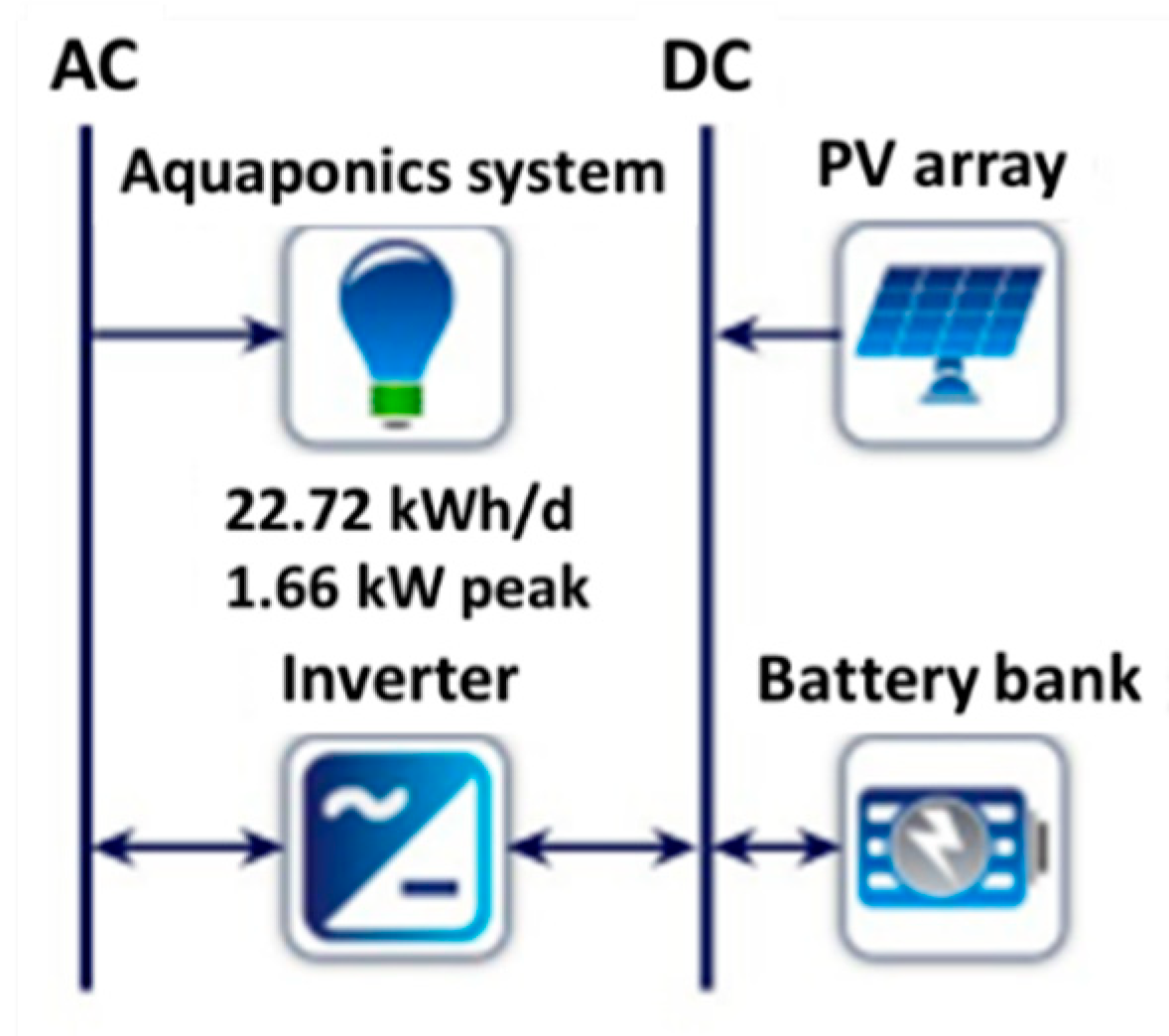
The energy flow of the stand-alone PVS is shown in Figure 10. The electricity supply is originally given by PV output (19,106 kWh) and battery storage depletion (about 29 kWh). It is obtained that the amount of electricity of 8291 kWh is consumed by the OCAS. If the amount of PV power generation is more than total amount of power demand and battery charging, the excess electricity is supplied to the dump load at that time. It is found that the excess electricity transferred to the dump load is 43% (8278 kWh) of the total PV power generation. However, this also implies that if the power demand of OCAS or storage capacity of PVS is reasonably increased, it is possible to spend the excess electricity for other operations instead of being transferred to the dump load. Therefore, it results in improving the energy use efficiency of the system [40].

3.2. Operating Performance of PVS Components

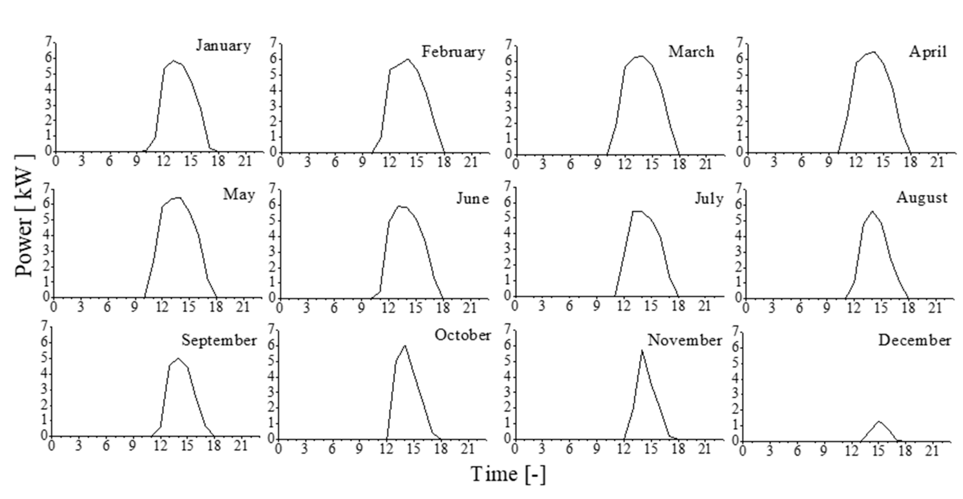
A summary data of the technical and economic performance of PV array, battery bank and inverter is shown in Table 6. The operation hours for PV power generation is 4156 h and the annual PV power generation is 19,106 kWh. The average power output of the PV array is 2.18 kW, and the average daily accumulated power generation is 52.32 kWh. The levelized cost for the PV array is $0.066/kWh. The levelized cost of the battery bank is not calculated because the battery bank is charged by the only the PV array. However, the battery wear cost of $0.196/kWh becomes significantly higher, calculating close to 45% of the COE ($0.438/kWh) (the simulated value of COE is explained in Section 3.4). The battery cost is more expensive than that of the PV array, which explains why users sometimes stop utilizing the battery bank and install more solar panels [41]. This leads to reduction in the initial equipment cost for system design of PVS to the same power demand. However, in the OCAS process, the circulation pump and the aeration pump must be worked for rearing the fish and the dehumidifier is also operated for recovering water from the air through the nighttime. Consequently, it must give preference to install more battery banks for ensuring the safe power supply although it results in increasing the equipment cost [42]. It is also simulated that the capacity of the inverter of the optimum PVS is 3.8 kW. The actual output of the inverter changes with power consumption of the OCAS. According to the simulation results, the annual amount of electricity imported to the inverter was 8821 kWh, and the annual amount of electricity exported from the inverter was 8291 kWh. The average output of the inverter was 0.947 kW with a minimum output of 0.135 kW and maximum output of 1.66 kW.

3.3. Technical and Economic Analysis of the PVS

3.3.1. Power Generation Characteristics of the PV Array

Figure 11 shows hourly profile of the power generation output of the PV array and Figure 12 shows the monthly total amount of power generation and the monthly average daily power generation of each month. In Figure 11, the PV power generation occurs typically from 7:00 a.m. and 6:00 pm in a day. The daily total time of power generation is about 12 h from the 30th day to the 240th day of the year and the time for the rest of the days is slightly shortened. In Figure 12, the monthly total amount of PV power generation and the monthly average daily PV power generation increase from January to May, and then decrease gradually from September to December. The decrease of the power output with seasonal meteorological condition is focused on because there is usually dry season and rainy season in dryland [43]. Moreover, in La Paz, Mexico, the seasonal typhoon in September (around 240th days) and the continuous cloudy days in December (330th days to 365th days) resulted in a decrease in solar radiation. This leads to an excessive decline in PV power generation. Even in drylands, the sizing of stand-alone PVS must be designed in consideration with not only average solar irradiation but also autonomy based on the number of infrequent and continuous cloudy days through a year. From this point, a hybrid power generation system can be considered as useful option, combining PV power with other renewable energy, such as wind power. According to the previous research [44,45], it is reported the COE of hybrid power generation system is smaller than that of PVS. However, the initial cost of the hybrid power generation system increases to a certain extent the initial cost of PVS, and the NPC will also increase. Therefore, when the power generation system is designed, it should also be compatible with local energy resources [46] and consider the increase of initial cost.

3.3.2. Operating Characteristics of the Battery Bank

The simulation results of the state of charge (SOC) of the battery bank in the stand-alone PVS are shown from Figure 13, Figure 14 and Figure 15. As shown in Figure 13 and Figure 14, the SOC of the battery bank changes between 60% and 100% in about 99.4% of the time in a given year (assuming that the battery bank discharges from a full charge (SOC 100%) at 0:00 a.m. on 1 January). It is also found that the SOC of the battery bank is more than 80% in 70.4% of the time in a given year, and the battery bank was in a “shallow” discharge state for most of the time. As shown in Figure 13 and Figure 15, a deep discharge occurred during nighttime in just two months. The lowest SOC values generated in September and December were 53.6% and 50.4%, respectively, with monthly average SOC values of 83.9% and 76.1%. As mentioned in Section 3.3.1, this is explained by the relatively unstable and insufficient solar irradiation caused by hurricanes in September and by continuous cloudy days in December. According to the simulation results shown in Table 6, the usable nominal capacity of battery banks is 54.3 kWh, which can support the operation of OCAS by only battery bank without PV power output for 57.4 h (autonomy: 2.4 days). The proposed PVS can ensure the smooth operation of OCAS mostly under the solar irradiation data in the current study. However, it is often performed to design the practical sizing of a stand-alone PVS with several values of autonomy in range of 3 to 5 [47,48]. In the actual operation of OCAS, it is difficult to predict the weather change every day accurately. On the basis of this study, the preparation of emergency generator for power supply may be recommended to ensure the safe operation of OCAS in the continuous occurrence of extreme weather. If the change of local seasonal solar irradiation is predicted, it can be suggested to carry out the maintenance of the OCAS equipment with the arrangement of fish raring schedule as the countermeasure for avoiding short-term power shortage.

3.3.3. Occurrence of Excess Power

When using a stand-alone PVS, the excess electricity is generated because of the mismatch between the periods of the PVS power generation and the OCAS power consumption. Rational use of excess power is one of the issues in the deployment of the PVS. The simulation was conducted using HOMER to clarify the power supply–demand relationship of the PVS every hour for a year. As mentioned in Section 3.2, the surplus power generation was found to be 8278 kWh, but those detailed results are shown from Figure 16 to Figure 18. As shown in Figure 16 and Figure 17, the statistics is conducted on the hourly excess power of each month. It is found that excess power is generated between 10:00 a.m. and 6:00 p.m. from January to July, and the maximum excess power is obtained around noon. On the other hand, it should be remarked to occur the continuous day without the excess power in September (around 240th days) and December (330th days to 365th days). Although the PVS power generation can meet the power demand of OCAS, it is not enough to fully charge the battery bank for this period, as mentioned in Section 3.3.2. It is actually required to monitor the power generation and SOC of the PVS. As shown in Figure 18, the monthly total amount of excess power and the monthly average of daily accumulated excess power decrease steadily from January to December, and they are extremely small for December. The COE is calculated by dividing the cost of the stand-alone PVS by the amount of power consumption of OCAS that is supplied by the PVS [49]. Thus, the COE could be further reduced by rationalizing the excess power and converting it to power consumption. For example, it is considered to regulate water temperature in aquaculture tank. Moreover, it is available to refrigerate fish and vegetables in postharvest processing on site.

3.4. Economic Evaluation of the PVS

In this study, the cost of the stand-alone PVS was evaluated using the total NPC and the levelized COE [50]. The total NPC of 
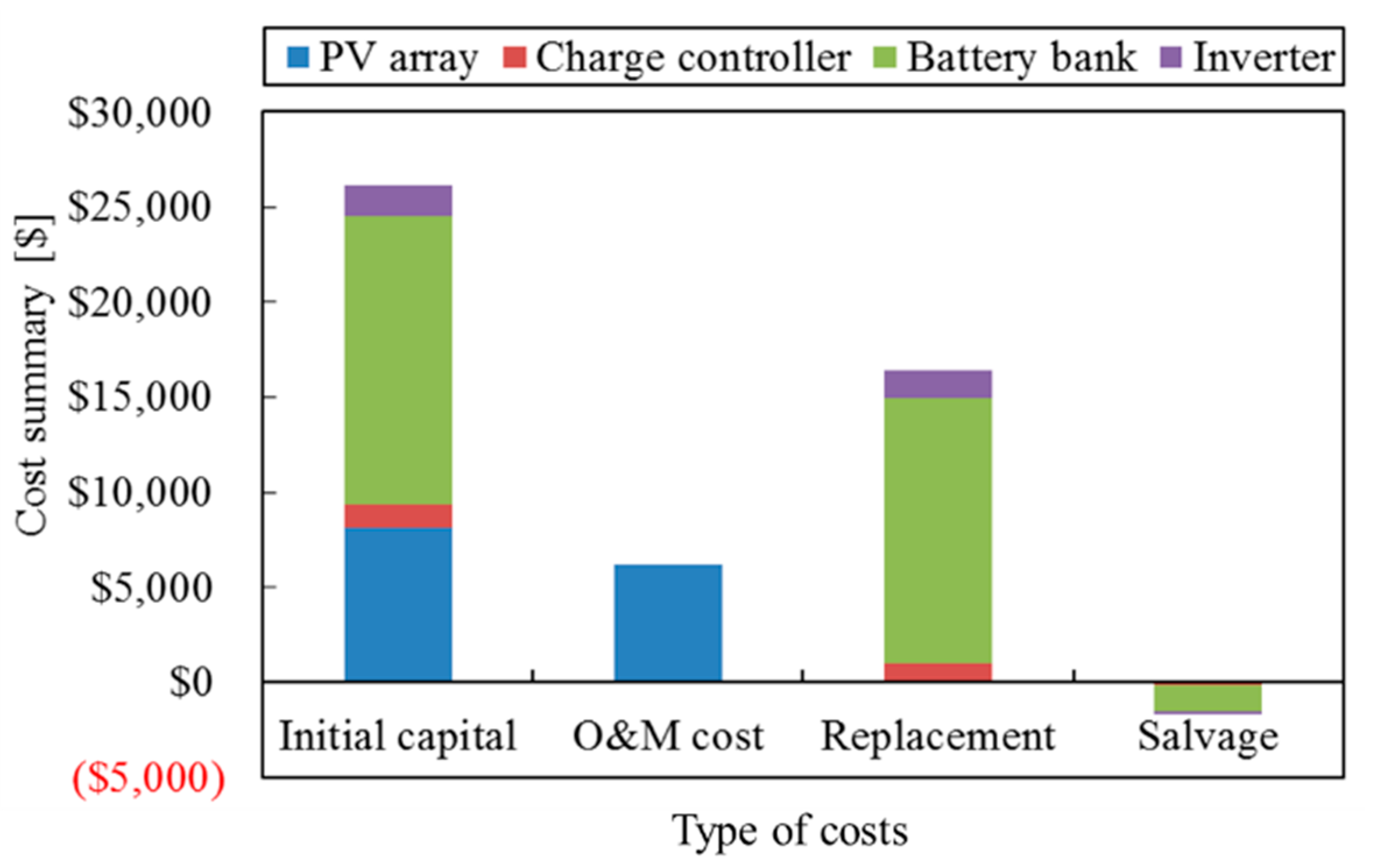
$46,993 for the proposed PVS is obtained from this simulation. Especially, the total NPC includes several types of cost such as initial capital, O&M, replacement and so on. The breakdown of NPC by type of cost and equipment for the PVS is shown in Figure 19. It is found that the initial capital cost of the PV system is $26,115 and reaches to about 56% of the total NPC. It is also remarkable that the cost for the battery bank reaches to about 59% through initial capital and replacement cost. This indicates that the cost of the power storage system in a stand-alone PVS is dominant. The cost of the 12.5 kW PV array occurs at the initial capital and O&M cost. It accounts for 31% of the total NPC of the PVS, while the cost of the inverter accounts for about 6% of the NPC of the entire system. The lowest cost item is the charge controller, which accounted for 4% of the NPC. At the end of the 25-year project, a total remaining value of $1696 for each facility is calculated.
It is also obtained that the COE of the PVS is $0.438/kWh, which is more than the current Mexican electricity rate ($0.221/kWh) [22]. However, because there is no power grid in the remote areas of drylands, comparing the COE of the PVS with the electricity cost of the areas with power grids may not reflect the actual costs of building the PVS. However, compared with a similar study [34], the COE is still in a reasonable range, which is economically advantageous [50] compared with the erection of long-distance transmission lines and utilization of diesel generators [51]. When calculating COE through Equation (4), the amount of excess power was not considered in the amount of “total electrical load served per year”. In the same PVS, even if the cost is constant and the power consumption (“total electrical load served per year”) is larger than that in current simulation, it is possible to reduce COE. According to the results explained in Section 3.1, 43% of the generated power is transferred to the dump load as excess power, which is not provided to the OCAS. The simulations of power supply and demand in Section 3.3.3 show that the system generates excess power during the day. It is suggested that the selection of electrical appliances or the setting of the service time of electrical appliances in the PVS must be considered, and the surplus electricity should be reasonably used to further reduce the COE.
OCAS operators bear certain economic risks due to the high equipment investment and meticulous production technology. Therefore, to guide the reasonable operation of the OCAS, it is very important to establish an effective operation and management method of the OCAS suitable for the operators themselves. The specific management strategy of the OCAS is uncovered in this study. To provide a reference for operators, the production and sales volume of OCAS through field empirical experiments is estimated and discussed below.
Previous researchers systematically conducted LCA and economic analysis of the whole aquaponic systems [52,53,54,55]. According to previous studies, the market price changes on vegetables and fish are in the range of $1.46–2.50/lb ($0.66–1.13/kg) and $1.46–5.00/lb ($0.66–2.27/kg), respectively. The production costs reported for vegetables and fish are $0.75–1.50/lb ($0.34–0.68/kg) and $1.46–4.99/lb ($0.66–2.26/kg), respectively. However, as mentioned in the introduction of this paper, the productivity and energy consumption of the aquaponic system are related to the structure, the scale and the local environment. The design and operation methods of aquaponics also affect the production. Therefore, it is difficult to use the existing data in this work. Instead, a simple economic estimation by referring to the data of local surveys and production data of unpublished empirical experiments in La Paz is achieved. According to the field empirical experiment, taking the OCAS shown in Section 2.1 as the research object, it can be estimated that the annual harvest is 225 kg tilapia, 78 kg Swiss chard and 48 kg pepper. Based on the market price survey data of fish and vegetables implemented in La Paz, the average sales prices in the last three years for tilapia, Swiss chard and pepper are respectively 51.80 pesos/kg ($2.23/kg), 24.13 pesos/kg ($1.04/kg) and 93.18 pesos/kg ($4.01/kg). Therefore, it can be estimated that the annual sales revenue is $775.35 (Tilapia: $501.75, Swiss chard: $81.12, Pepper: $192.48). Assuming that the commodity price of these remains unchanged, the sales revenue will be $19,383.75 within 25 years. If the sales revenue of 25 years is changed to NPC, further reduction of the total NPC may be expected. However, the cost of power equipment let alone the overall material and labor costs is much higher than the sales revenue of the OCAS system.
From the perspective of sales revenue of harvests, it seems even less economical to set up a stand-alone PVS for OCAS. However, compared with the previous aquaponics, OCAS can not only produce food but also alleviate the salinization of soil. In addition, the stand-alone PVS using clean energy has a series of beneficial effects on reducing greenhouse gas emissions [56]. The important impact of the PVS on the environment should also be positively evaluated. In addition, if OCAS has a stand-alone power supply device, the applicability of OCAS in remote areas will be greatly promoted. Therefore, it is difficult to simply evaluate the budgeting of this system by only looking at the sales revenue. Combined with the values of environmental protection and mitigation of food shortage, the evaluation of the economic and environmental benefits of the whole system is a topic of future work.

4. Conclusions

Food security in drylands is a major concern due to rapid population growth. The depletion of groundwater for irrigated agriculture and soil degradation due to the use of highly saline groundwater worsen food production and productivity in these regions. To achieve both effective water use and prevention of soil salinization, the OCAS was established. Moreover, to achieve sustainable production of the OCAS in remote areas without power supply, a stand-alone PVS was designed. To promote the utilization of the OCAS in these remote areas, the techno-economic feasibility of optimum stand-alone PVS that can supply electricity for aquaponic systems was discussed.
HOMER software was employed to perform simulations and techno-economic evaluation of the stand-alone PVS for the pilot system of the OCAS installed in CIBNOR, La Paz, Baja California Sur, Mexico. It was found that the average daily GHI was 6.12 kWh/m2, which is suitable for PV power generation. The total NPC of the stand-alone PVS was calculated as $46,993, and the capacity of each component was derived as 12.5 kW of PV array, 8 kW of charge controller, 40 units of battery and 3.8 kW of inverter. The cost of the battery bank, PV array, inverters and charge controllers were also found to account for 59%, 31%, 6% and 4% of the NPC for the proposed stand-alone PVS, respectively. In addition, the COE of the PVS was calculated to be $0.438/kWh. Furthermore, the annual power supply and demand of the proposed stand-alone PVS were analyzed. The power generation of PV array was performed for 4156 h and was estimated power generation of 19,106 kWh annually. Furthermore, 43% of the generated power was transferred to the dump load as excess power, which was not supplied to the OCAS. The power supply and demand simulations showed that the excess power of the system occurred in almost every afternoon. Therefore, COE can be further reduced by rationally consuming excess power during OCAS operation.
The number of days for low solar irradiation were 5 days (February), 8 days (September) and 10 days (December), respectively. It is explained that the full charging of battery bank cannot be achieved for these periods. The autonomy of the proposed PVS was presented for 2.4 days. The PVS operation with the low SOC condition is a risk that leads to cutting off the power supply for the OCAS. The preparation of countermeasure for ensuring power supply and safe operation of OCAS in the continuous occurrence of low solar radiation is recommended, even on dryland.
In conclusion, this study provides insight into optimizing a stand-alone low-cost PVS to provide power supply for aquaponics on drylands. To successfully guide the operation of the OCAS, it is necessary to examine production technology and management methods. Based on the achievement of breeding and cultivation technology for the OCAS not only the optimization of the PVS but also the overall operation management of the OCAS can be achieved.

Author Contributions

Conceptualization, K.T.; Formal analysis, B.B.; Funding acquisition, K.T. and J.G.; Investigation, K.T. and J.G.; Methodology, K.T.; Software, B.B.; Supervision, K.T.; Writing—original draft, B.B.; Writing—review and editing, B.B., K.T. and J.G. All authors have read and agreed to the published version of the manuscript.

Funding

This research was funded by the Japan Science and Technology Agency (JST)/Japan International Cooperation Agency (JICA), grant number JPMJSA1405.

Acknowledgments

This research was supported by the Japan Science and Technology Agency (JST)/Japan International Cooperation Agency (JICA), Science and Technology Research Partnership for Sustainable Development (SATREPS) program.

Conflicts of Interest

The authors declare no conflict of interest.

References

  1. Food and Agriculture Organization (FAO). Status and trends in land and water resources. In The State of the World’s Land and Water Resources for Food and Agriculture-Managing Systems at Risk; Food and Agriculture Organization of the United Nation: Rome, Italy; Earthscan: London, UK, 2011; pp. 19–62. [Google Scholar]
  2. Rosenzweig, C.; Parry, M.L. Potential impact of climate change on world food supply. Nature 1994, 367, 133–138. [Google Scholar] [CrossRef]
  3. Food and Agriculture Organization (FAO). The State of Food and Agriculture. Innovation in Family Farming; Food and Agriculture Organization of the United Nations: Rome, Italy; Earthscan: London, UK, 2014. [Google Scholar]
  4. Gaffney, J.; Bing, J.; Byrne, P.F.; Cassman, K.G.; Ciampitti, I.; Delmer, D.; Habben, J.; Lafitte, H.R.; Lidstrom, U.E.; Porter, D.O.; et al. Science-based intensive agriculture: Sustainability, food security, and the role of technology. Glob. Food Sec. 2019, 23, 236–244. [Google Scholar] [CrossRef]
  5. Abdul-Rahman, S.; Saoud, I.P.; Owaied, M.K.; Holail, H.; Farajalla, N.; Haidar, M.; Ghanawi, J. Improving water use efficiency in semi-arid regions through integrated aquaculture/agriculture. J. Appl. Aquac. 2011, 23, 212–230. [Google Scholar] [CrossRef]
  6. Brummett, R.E. Comparative analysis of the environmental costs of fish farming and crop production in arid areas. In FAO Fisheries Proceedings. No. 10, Proceeding of the FAO/WFT Expert Workshop, Comparative Assessment of the Environmental Costs of Aquaculture and Other Food Production Sectors: Methods for Meaningful Comparisons, Vancouver, Canada, 24–28 April 2006; FAO: Rome, Italy, 2007; pp. 221–228. [Google Scholar]
  7. Love, D.C.; Fry, J.P.; Genello, L.; Hill, E.S.; Frederick, J.A.; Li, X.; Semmens, K. An international survey of aquaponics practitioners. PLoS ONE 2014, 9, e102662. [Google Scholar] [CrossRef] [PubMed] [Green Version]
  8. Rakocy, J.E.; Masser, M.P.; Losordo, T.M. Recirculating aquaculture tank production systems: Aquaponics—Integrating fish and plant culture. In SRAC Publication; Kentucky Stste University: Frankfurt, KY, USA, 2006; No. 454. [Google Scholar]
  9. Saoud, I.P. Ensuring Food Security by Improving “Freshwater Use Efficiency” or by Farming the Seas. In Water, Energy & Food Sustainability in the Middle East; Badran, A., Murad, S., Baydoun, S., Daghir, N., Eds.; Springer International Publishing: Cham, Switzerland, 2017; pp. 341–360. [Google Scholar]
  10. Hu, Z.; Lee, J.W.; Chandran, K.; Kim, S.; Brotto, A.C.; Khanal, S.K. Effect of plant species on nitrogen recovery in aquaponics. Bioresour. Technol. 2015, 188, 92–98. [Google Scholar] [CrossRef]
  11. Knaus, U.; Palm, H.W. Effects of the fish species choice on vegetables in aquaponics under spring-summer conditions in northern Germany (Mecklenburg Western Pomerania). Aquaculture 2017, 473, 62–73. [Google Scholar] [CrossRef]
  12. Goddek, S.; Delaide, B.; Mankasingh, U.; Ragnarsdottir, K.V.; Jijakli, H.; Thorarinsdottir, R. Challenges of sustainable and commercial aquaponics. Sustainability 2015, 7, 4199–4224. [Google Scholar] [CrossRef] [Green Version]
  13. Love, D.C.; Uhl, M.S.; Genello, L. Energy and water use of a small-scale raft aquaponics system in Baltimore, Maryland, United States. Aquac. Eng. 2015, 68, 19–27. [Google Scholar] [CrossRef] [Green Version]
  14. Van Ginkel, S.W.; Igou, T.; Chen, Y. Energy, water and nutrient impacts of California-grown vegetables compared to controlled environmental agriculture systems in Atlanta, GA. Resour. Conserv. Recycl. 2017, 122, 319–325. [Google Scholar] [CrossRef]
  15. Qoaider, L.; Steinbrecht, D. Photovoltaic systems: A cost competitive option to supply energy to off-grid agricultural communities in arid regions. Appl. Energy 2010, 87, 427–435. [Google Scholar] [CrossRef]
  16. Mitra, I.; Chaudhuri, S.P.G. Remote village electrification plan through renewable energy in the Islands of Indian Sundarbans. Int. Sol. Energy Soc. UK Sect. Conf. C 2006, 85, 315. [Google Scholar]
  17. Fulhu, M.; Mohamed, M.; Krumdieck, S. Voluntary demand participation (VDP) for security of essential energy activities in remote communities with case study in Maldives. Energy Sustain. Dev. 2019, 49, 27–38. [Google Scholar] [CrossRef]
  18. Song, J. Super grid in North-East Asia through renewable energy. Asia Pac. Tech. Monit. 2014, 31, 24–27. [Google Scholar]
  19. Chel, A.; Kaushik, G. Renewable energy for sustainable agriculture. Agron. Sustain. Dev. 2011, 31, 91–118. [Google Scholar] [CrossRef]
  20. Yogev, U.; Barnes, A.; Gross, A. Nutrients and energy balance analysis for a conceptual model of a three loops off grid, aquaponics. Water 2016, 8, 589. [Google Scholar] [CrossRef] [Green Version]
  21. Japan Science and Technology Agency. Available online: https://www.jst.go.jp/global/english/kadai/h2605_mexico.html (accessed on 31 July 2020).
  22. Mundo-Hernández, J.; Alonso, B.C.; Hernández-Álvarez, J.; Celis-Carrillo, B. An overview of solar photovoltaic energy in Mexico and Germany. Renew. Sustain. Energy Rev. 2014, 31, 639–649. [Google Scholar] [CrossRef]
  23. Alemán-Nava, G.S.; Casiano-Flores, V.H.; Cárdenas-Chávez, D.L.; Díaz-Chavez, R.; Scarlat, N.; Mahlknecht, J.; Dallemand, J.F.; Parra, R. Renewable energy research progress in Mexico: A review. Renew. Sustain. Energy Rev. 2014, 32, 140–153. [Google Scholar] [CrossRef]
  24. Duffie, J.A.; Beckman, W.A. Solar Engineering of Thermal Processes, 4th ed.; John Wiley & Sons: Hoboken, NJ, USA, 2013; pp. 3–138. [Google Scholar]
  25. Trina Solar. Available online: https://static.trinasolar.com/sites/default/files/Datasheet-PD05.08.pdf (accessed on 18 July 2018).
  26. Outback Power Inc. Available online: http://www.outbackpower.com/downloads/documents/charge_controllers/flexmax_6080/specsheet.pdf (accessed on 18 July 2018).
  27. Trojan Battery Company. Available online: https://www.trojanbattery.com/pdf/datasheets/SPRE_12_225_DS.pdf (accessed on 18 July 2018).
  28. Al-Karaghouli, A.; Kazmerski, L.L. Optimization and life-cycle cost of health clinic PV system for a rural area in southern Iraq using HOMER software. Sol. Energy 2010, 84, 710–714. [Google Scholar] [CrossRef]
  29. Manwell, J.F.; McGowan, J.G. Lead acid battery storage model for hybrid energy systems. Sol. Energy 1993, 50, 399–405. [Google Scholar] [CrossRef]
  30. Upadhyay, S.; Sharma, M.P. Development of hybrid energy system with cycle charging strategy using particle swarm optimization for a remote area in India. Renew. Energy 2015, 77, 586–598. [Google Scholar] [CrossRef]
  31. Schneider Eelectric. Available online: https://solar.schneider-electric.com/product/sw-na/ (accessed on 18 July 2018).
  32. Adaramola, M.S.; Paul, S.S.; Oyewola, O.M. Assessment of decentralized hybrid PV solar-diesel power system for applications in Northern part of Nigeria. Energy Sustain. Dev. 2014, 19, 72–82. [Google Scholar] [CrossRef]
  33. Lau, K.Y.; Yousof, M.F.M.; Arshad, S.N.M.; Anwari, M.; Yatim, A.H.M. Performance analysis of hybrid photovoltaic/diesel energy system under Malaysian conditions. Energy 2010, 35, 3245–3255. [Google Scholar] [CrossRef]
  34. Bahramara, S.; Moghaddam, M.P.; Haghifam, M.R. Optimal planning of hybrid renewable energy systems using HOMER: A review. Renew. Sustain. Energy Rev. 2016, 62, 609–620. [Google Scholar] [CrossRef]
  35. Lambert, T.; Gilman, P.; Lilienthal, P. Micropower system modeling with HOMER. In Integration of Alternative Sources of Energy; Felix, A., Farret, F.A., Simoes, M.G., Eds.; John Wiley & Sons, Inc.: Hoboken, NJ, USA, 2005; pp. 379–418. [Google Scholar]
  36. Mahmud, N.; Hassan, A.; Rahman, M.S. Modelling and cost analysis of hybrid energy system for St. Martin Island using HOMER. In Proceedings of the 2013 International Conference on Informatics, Electronics and Vision (ICIEV), Dhaka, Bangladesh, 17–18 May 2013; pp. 1–6. [Google Scholar] [CrossRef]
  37. He, G.X.; Cheng, L.; Xu, J.; Chen, L.; Tao, W.Q. Optimal configuration of a wind/PV/battery hybrid energy system using HOMER software. Chem. Eng. Trans. 2017, 61, 1507–1512. [Google Scholar] [CrossRef]
  38. Murphy, P.M.; Twaha, S.; Murphy, I.S. Analysis of the cost of reliable electricity: A new method for analyzing grid connected solar, diesel and hybrid distributed electricity systems considering an unreliable electric grid, with examples in Uganda. Energy 2014, 66, 523–534. [Google Scholar] [CrossRef]
  39. Food and Agriculture Organization (FAO). Small-scale aquaponic food production: Integrated fish and plant farming. In FAO Fisheries and Aquaculture Technical Paper, 589; Food and Agriculture Organization of the United Nations: Rome, Italy, 2014. [Google Scholar]
  40. Sawle, Y.; Gupta, S.C.; Bohre, A.K. Review of hybrid renewable energy systems with comparative analysis of off-grid hybrid system. Renew. Sustain. Energy Rev. 2018, 81, 2217–2235. [Google Scholar] [CrossRef]
  41. Ma, T.; Yang, H.; Lin, L. A feasibility study of a stand-alone hybrid solar–wind–battery system for a remote island. Appl. Energy 2014, 121, 149–158. [Google Scholar] [CrossRef]
  42. Amrollahi, M.H.; Bathaee, S.M.T. Techno-economic optimization of hybrid photovoltaic/wind generation together with energy storage system in a stand-alone micro-grid subjected to demand response. Appl. Energy 2017, 202, 66–77. [Google Scholar] [CrossRef]
  43. Arnon, I. Agriculture in dry lands: Principles and practice; Elsevier: Amsterdam, The Netherlands, 1992; pp. 3–38. [Google Scholar]
  44. Goel, S.; Ali, S.M. Cost analysis of solar/wind/diesel hybrid energy systems for Telecom tower by using HOMER. Int. J. Renew. Energy Res. 2014, 4, 305–311. [Google Scholar]
  45. Halabi, L.M.; Mekhilef, S.; Olatomiwa, L.; Hazelton, J. Performance analysis of hybrid PV/diesel/battery system using HOMER: A case study Sabah, Malaysia. Energy Convers. Manag. 2017, 144, 322–339. [Google Scholar] [CrossRef]
  46. Mondal, M.A.H.; Denich, M. Assessment of renewable energy resources potential for electricity generation in Bangladesh. Renew. Sustain. Energy Rev. 2010, 14, 2401–2413. [Google Scholar] [CrossRef]
  47. Gopi, N.P.; Devendran, S. Autonomy considerations for a standalone photovoltaic system. Sustain. Energy Technol. Assess. 2015, 10, 79–83. [Google Scholar]
  48. Kaplani, E.; Kaplanis, S. A stochastic simulation model for reliable PV system sizing providing for solar radiation fluctuations. Appl. Energy 2012, 97, 970–981. [Google Scholar] [CrossRef]
  49. Haidar, A.M.; John, P.N.; Shawal, M. Optimal configuration assessment of renewable energy in Malaysia. Renew. Energy 2011, 36, 881–888. [Google Scholar] [CrossRef] [Green Version]
  50. Branker, K.; Pathak, M.J.M.; Pearce, J.M. A review of solar photovoltaic levelized cost of electricity. Renew. Sustain. Energy Rev. 2011, 15, 4470–4482. [Google Scholar] [CrossRef] [Green Version]
  51. Ouedraogo, B.I.; Kouame, S.; Azoumah, Y.; Yamegueu, D. Incentives for rural off grid electrification in Burkina Faso using LCOE. Renew. Energy 2015, 78, 573–582. [Google Scholar] [CrossRef]
  52. Engle, C.R. Economics of aquaponics. In SRAC Publication; Kentucky Stste University: Frankfurt, KY, USA, 2015; No. 5006. [Google Scholar]
  53. Tokunaga, K.; Tamaru, C.; Ako, H.; Leung, P.S. Economics of small-scale commercial aquaponics in Hawai‘i. J. World Aquac. Soc. 2015, 46, 20–32. [Google Scholar] [CrossRef]
  54. Baker, A. Preliminary Development and Evaluation of an Aquaponic System for the American Insular Pacific. Ph.D. Thesis, University of Hawaii at Manoa, Honolulu, HI, USA, 2010. Available online: https://scholarspace.manoa.hawaii.edu/handle/10125/101649 (accessed on 3 September 2020).
  55. Quagrainie, K.K.; Flores, R.M.V.; Kim, H.J.; McClain, V. Economic analysis of aquaponics and hydroponics production in the U.S. Midwest. J. Appl. Aquac. 2018, 30, 1–14. [Google Scholar] [CrossRef]
  56. Tsoutsos, T.; Frantzeskaki, N.; Gekas, V. Environmental impacts from the solar energy technologies. Energy Policy 2005, 33, 289–296. [Google Scholar] [CrossRef]
Figure 1. Water flow and equipment location of an open-field cultivation combined-type aquaponic system (OCAS).
Sustainability 12 09556 g001
Figure 2. Details of power consumption of the OCAS in a day.
Sustainability 12 09556 g002
Figure 3. Monthly average daily global horizontal irradiation (GHI) and clearness index in 2017.
Sustainability 12 09556 g003
Figure 4. Variation of annual power generation with tilt angle of 1 kW output photovoltaic (PV) panel.
Sustainability 12 09556 g004
Figure 5. Daily solar irradiation on surface at a tilt angle of 22° throughout 2017.
Sustainability 12 09556 g005
Figure 6. Monthly total solar irradiation and monthly average daily solar irradiation in 2017.
Sustainability 12 09556 g006
Figure 7. Schematic of a stand-alone photovoltaic system (PVS) for the OCAS.
Sustainability 12 09556 g007
Figure 8. Optimization results sorted by total net present cost (NPC).
Sustainability 12 09556 g008
Figure 9. System configuration of the proposed PV system with battery storage in HOMER.
Sustainability 12 09556 g009
Figure 10. Energy flow of the proposed PVS.
Sustainability 12 09556 g010
Figure 11. Hourly profile of simulated PV array output during 2017.
Sustainability 12 09556 g011
Figure 12. Monthly total PV power generation and monthly average daily PV power generation.
Sustainability 12 09556 g012
Figure 13. Hourly profile of simulated battery bank state of charge during 2017.
Sustainability 12 09556 g013
Figure 14. Relative frequency of SOC.
Sustainability 12 09556 g014
Figure 15. Boxplot of SOC in each month.
Sustainability 12 09556 g015
Figure 16. Hourly profile of simulated excess power during 2017.
Sustainability 12 09556 g016
Figure 17. Variation of average excess power with time by month.
Sustainability 12 09556 g017
Figure 18. Monthly total excess power generation and monthly average daily excess power generation.
Sustainability 12 09556 g018
Figure 19. Breakdown of NPC by component and cost type.
Sustainability 12 09556 g019
Table 1. Electrical equipment in the OCAS.
SectionEquipment (Quantity)PowerOperating Time
AquacultureAir pump (1)25 W24 h/day
Circulation pump (1)60 W24 h/day
UV sterilizer (1)20 W24 h/day
Hydroponic Circulation pump (1)30 W24 h/day
Open-field cultivation Irrigation pump (1)160 W10:30–10:55
OthersLED lighting (4)18 W20:00–20:30
Dehumidifier (2)745 W19:00–8:00
Potable water pump (2)60 WOnce every 30 days
11:00–11:50
12:00–12:50
Table 2. Specifications of PV array.
ManufacturerTrina Solar
ModelTSM-260 PD 05.08
Rated output under standard test condition260 W
Temperature coefficient−0.41%/°C
Normal operating cell temperature44 °C
Efficiency under standard test condition15.9%
Capital cost$170/panel
Replacement cost$170/panel
Operating and maintenance (O&M) cost per panel$10/year
Derating factor0.8
Tilt angle22°
Lifetime25 years
Search condition of PV capacity in HOMER1–100 panels (with an interval of 1)
Table 3. Specifications of a charge controller.
ManufacturerOutBack Power
ModelFLEXmax 80
Nominal battery voltage48 VDC
Maximum input voltage150 VDC
Maximum output current80 A
Maximum output4000 W
Efficiency97.5%
Capital cost$580/unit
Replacement cost$580/unit
O&M cost$0
Lifetime10 years
Search condition in HOMER1–6 units (with an interval of 1)
Table 4. Specifications of a battery bank.
ManufacturerTrojan
ModelSPRE 12 225
Rated capacity2.71 kWh
Maximum capacity226 Ah
Rated output voltage12 V
Roundtrip efficiency80%
Maximum depth of discharge50%
Capital cost$379/unit
Replacement cost$379/unit
O&M cost$0
Lifetime throughput2172 kWh
Search condition of battery bank capacity in HOMER4–80 units (with an interval of 4)
Table 5. Specifications of inverter.
ManufacturerSchneider
ModelConext SW4048
Rated output capacity3.8 kW
Lifetime10 years
Efficiency94.0%
Capital cost$1595/unit
Replacement cost$1595/unit
O&M cost$0
Search condition in HOMER1–6 units (with an interval of 1)
Table 6. Component performances of the proposed stand-alone PVS during the simulated year.
PV ArrayBattery BankInverter
Rated capacity12.5 kWBatteries number40 unitsCapacity3.8 kW
Mean output2.18 kWUsable nominal capacity54.3 kWhCapacity factor24.9%
Capacity factor17.5%Battery wear cost$0.196/kWhMean output0.947 kW
Total production19,106 kWh/yearAnnual throughput9122 kWh/yearMinimum output0.135 kW
Hours of operation4156 h/yearExpected life9.52 yearMaximum output1.66 kW
Levelized cost$0.066/kWhAutonomy57.4 hHours of operation8760 h/year
Minimum output0 kWEnergy in10,165 kWh/yearEnergy in8821 kWh/year
Maximum output8.00 kWEnergy out8159 kWh/yearEnergy out8291 kWh/year
Publisher’s Note: MDPI stays neutral with regard to jurisdictional claims in published maps and institutional affiliations.

