Active Distribution Network Modeling for Enhancing Sustainable Power System Performance; a Case Study in Egypt

Abstract

The remarkable growth of distributed generation (DG) penetration inside electrical power systems turns the familiar passive distribution networks (PDNs) into active distribution networks (ADNs). Based on the backward/forward sweep method (BFS), a new power-flow algorithm was developed in this paper. The algorithm is flexible to handle the bidirectional flow of power that characterizes the modern ADNs. Models of the commonly used distribution network components were integrated with the developed algorithm to form a comprehensive tool. This tool is valid for modeling either balanced or unbalanced ADNs with an unlimited number of nodes or laterals. The integrated models involve modeling of distribution lines, losses inside distribution transformers, automatic voltage regulators (AVRs), DG units, shunt capacitor banks (SCBs) and different load models. To verify its validity, the presented algorithm was first applied to the unbalanced IEEE 37-node standard feeder in both passive and active states. Moreover, the algorithm was then applied to a balanced 22 kV real distribution network as a case study. The selected network is located in a remote area in the western desert of Upper Egypt, far away from the Egyptian unified national grid. Accordingly, the paper examines the current and future situation of the Egyptian electricity market. Comparison studies between the performance of the proposed ADNs and the classical PDNs are discussed. Simulation results are presented to demonstrate the effectiveness of the proposed ADNs in preserving the network assets, improving the system performance and minimizing the power losses.

1. Introduction

Electrical power system modeling is a significant approach for the optimization of planning, designing or operating that system technically and economically. Therefore, the invention of the digital computer in the 1940s encouraged scholars to start solving different network troubles by different algorithms and techniques [1,2,3,4,5,6,7,8]. Many algorithms such as the Newton–Raphson (NR), Gauss–Seidel (GS) and fast decoupled (FD) are appropriately validated for simulating transmission systems (TSs) [4,5,6,7,8]. Nevertheless, the distribution systems are distinguished in numerous features. High values of the resistance-to-reactance ratio, R/X, are distinctive in distribution voltage levels while these values are decreasing as the voltage level increases in TSs. All TSs consist of tightly meshed networks whereas distribution systems may have radial or weakly meshed configurations. Generator nodes in distribution systems may be PQ, PV or composite nodes while generator nodes in transmission systems are mostly PV nodes. The PQ node is the node at which voltage can be regulated by controlling the real and reactive powers (P and Q) independently. PV node is the node at which generated real power and voltage magnitude (P and V) can be controlled independently.

Table 1. Assessment of distribution and transmission power systems.

Feature	Distribution System	Transmission System
Structure	Radial/Weakly meshed	Tightly meshed
Types of Load	Constant Power (CP)/Constant Current (CC)/Constant Impedance (CI)/Composite	Mostly CP only
Symmetricity	Unbalanced/Balanced	Balanced
R/X Ratio	High	Very low
Generator Nodes	PQ/PV/Composite	Mostly PV only

itemizes the differences between distribution and transmission power systems concerning the power flow analysis. Accordingly, conventional presented algorithms may not be suitable for solving the problems of radial distribution networks (DNs) with an acceptable convergence [9,10,11,12,13,14,15]. The distinctive radial structure of DNs is used as a basic feature to simulate DNs using the technique known as backward/forward sweep (BFS) [16,17,18,19].

Recently, distribution utilities have faced new challenges concerning environmental conservation, power sustainability and energy market economics. Therefore, a remarkable growth in the penetration rate of distributed generation (DG) units inside power DNs has been informed [20]. This growth turns the classical passive distribution networks (PDNs) into active distribution networks (ADNs) concerning the bidirectional flow of power [21,22,23]. A popular definition of the ADN was presented in [24] by the CIGRE working group C6.19. The new topology of ADNs necessitates modern simulation of network impedances under different grid conditions [25,26]. The newly added components lead to the need of modeling balanced and/or unbalanced ADNs using grid-connected inverters [27]. Reference [28] presents a review of power distribution planning models in ADNs where a lack of modeling networks containing an automatic voltage regulator (AVR) as a voltage control unit is noticed. Moreover, the previously presented models neglect one important source of losses in real DNs, namely power dissipated inside distribution transformers. This paper tries to fill this gap and presents a comprehensive power-flow program based on the BFS technique. The program is embedded with models of the commonly used DN components.

In this paper, a real Egyptian DN is highlighted as a practical application of the proposed program. The current and future situation of the Egyptian electricity market is examined in Section 2 focusing on the case-study region. Section 3 presents the modeling of distribution lines, losses inside distribution transformers, AVR groups, DG units, shunt capacitor banks (SCBs) and different load models. The integration of these models with the proposed power-flow algorithm is described in Section 4. Simulation results are discussed in Section 5 focusing on the analysis of two different networks before and after their conversion to ADNs. Eventually, Section 6 summarizes the main conclusions.

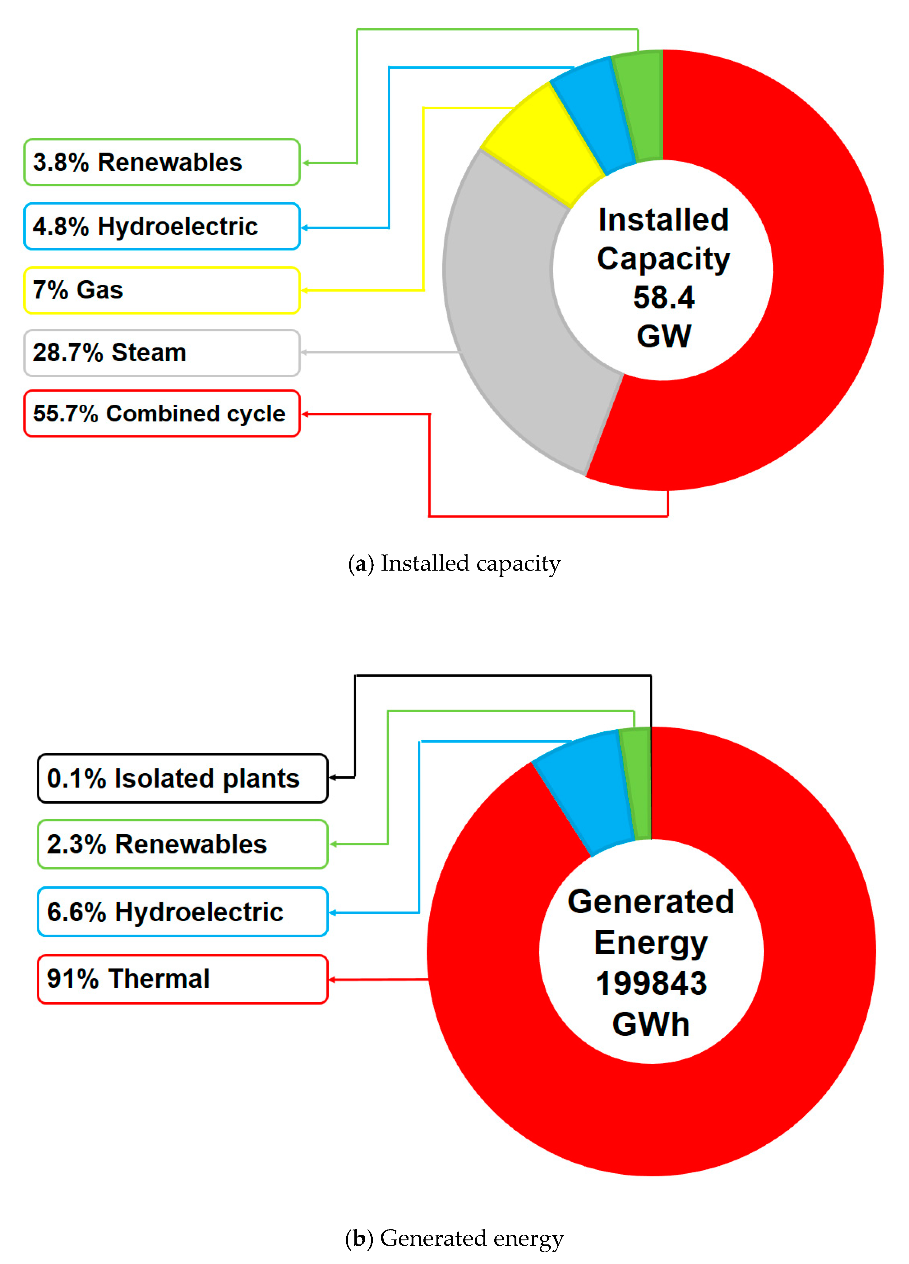
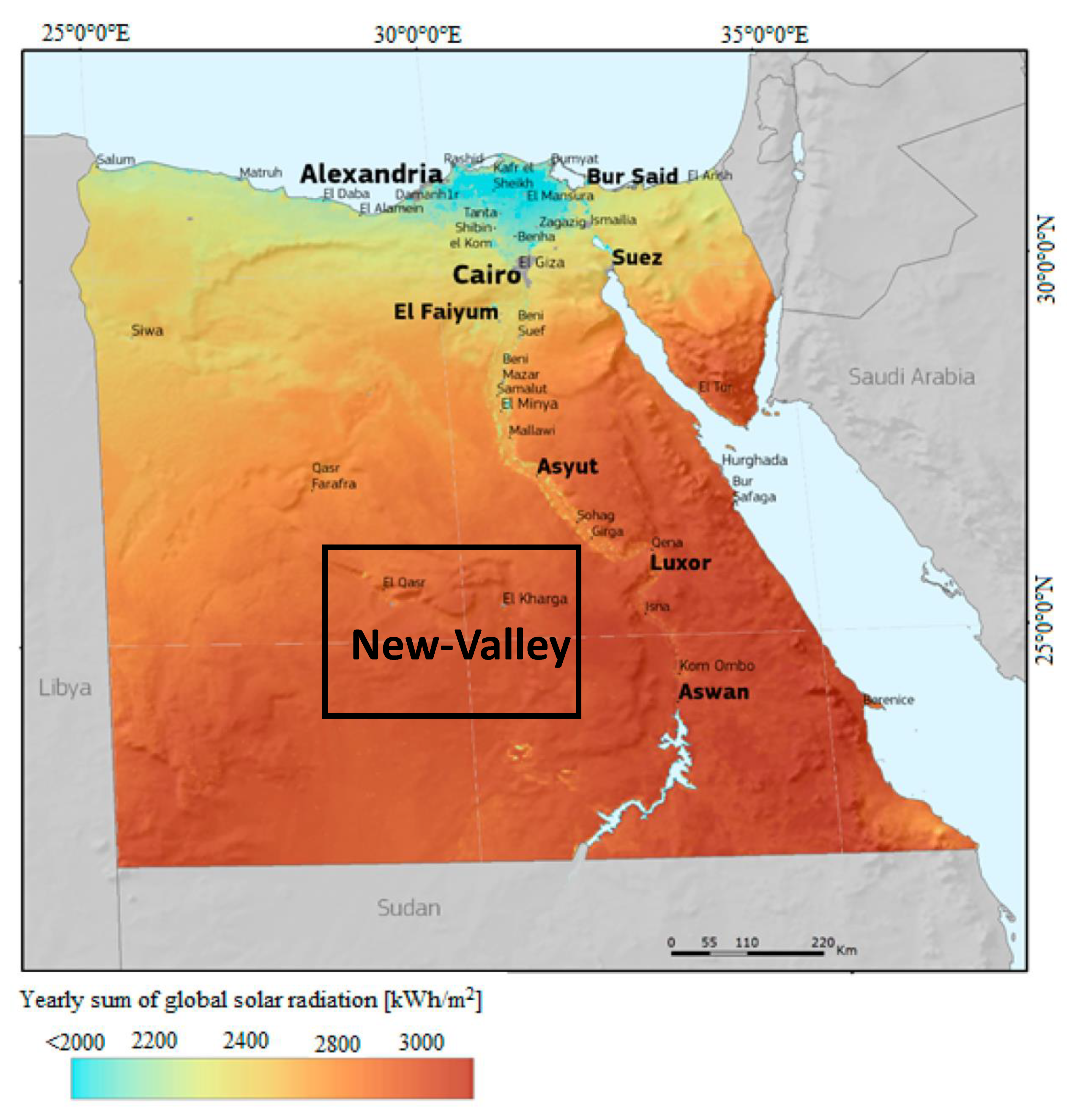
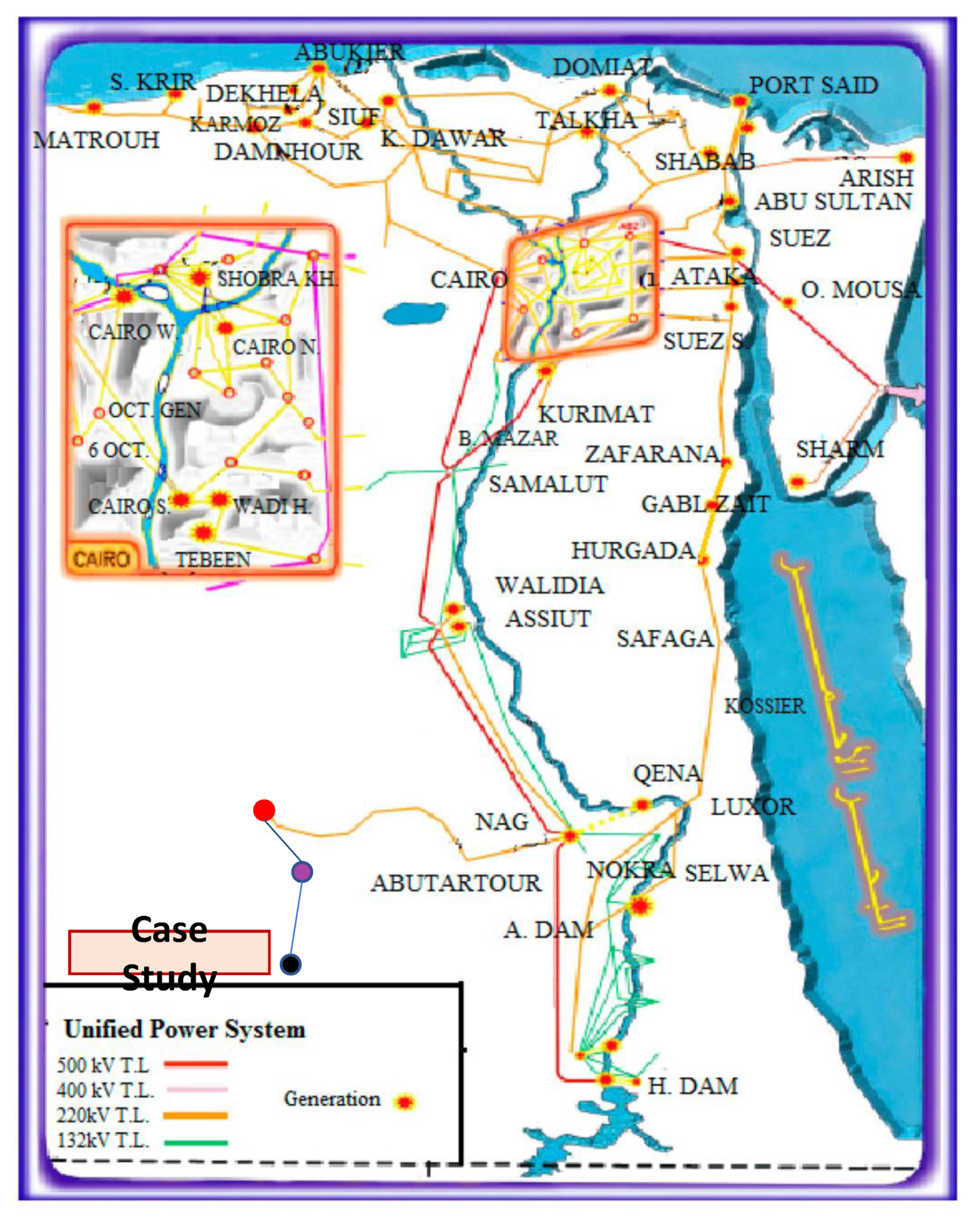
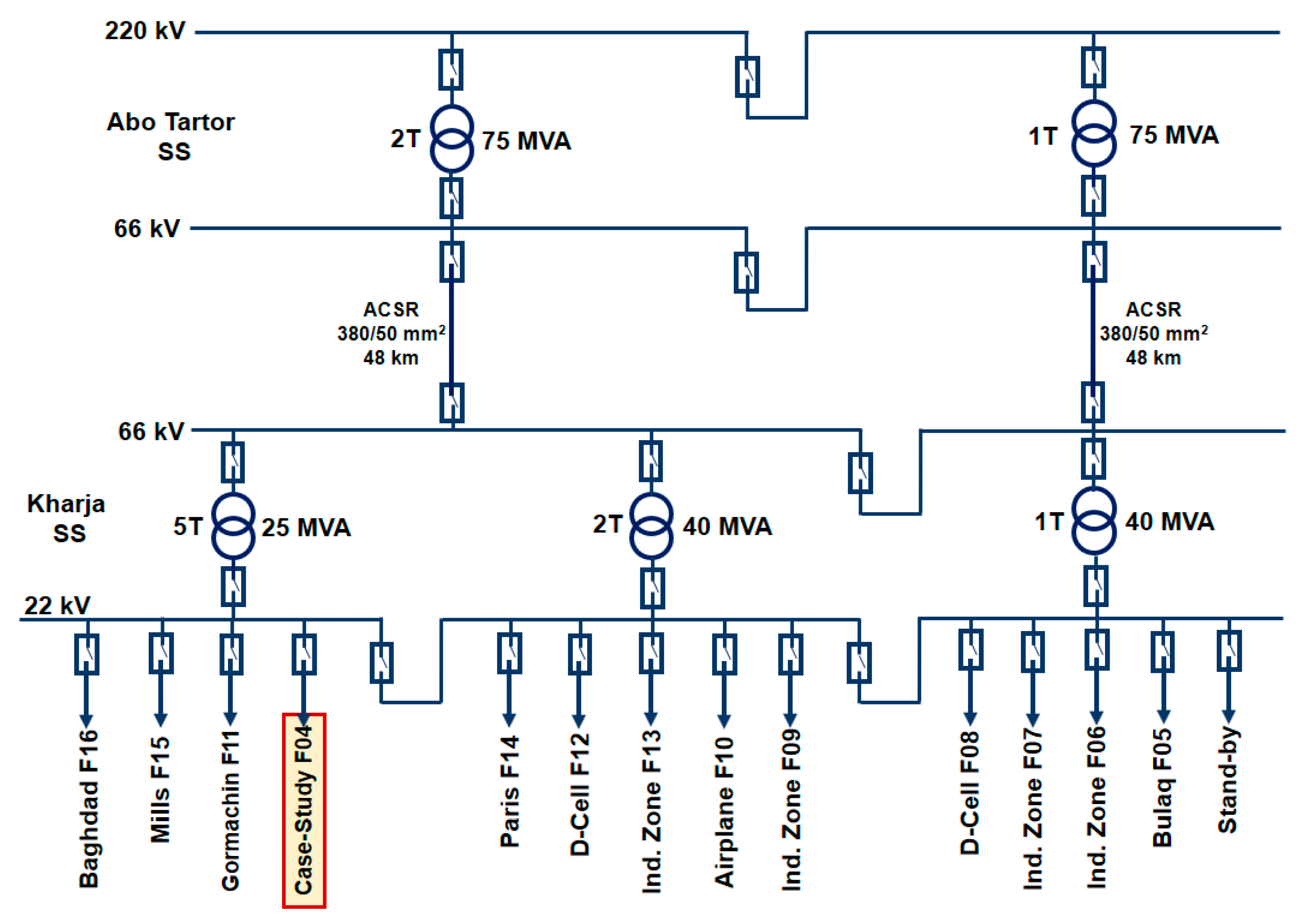
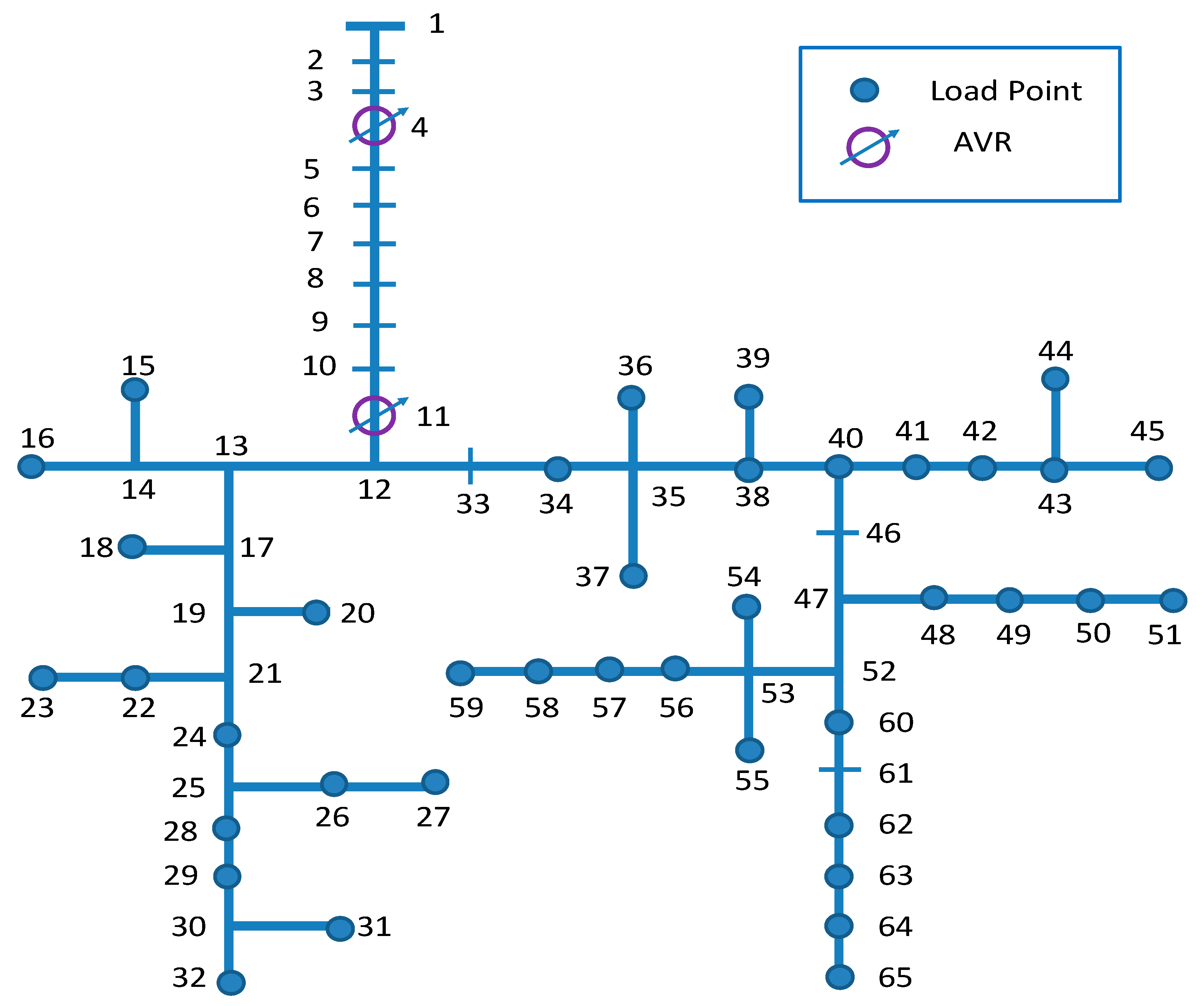
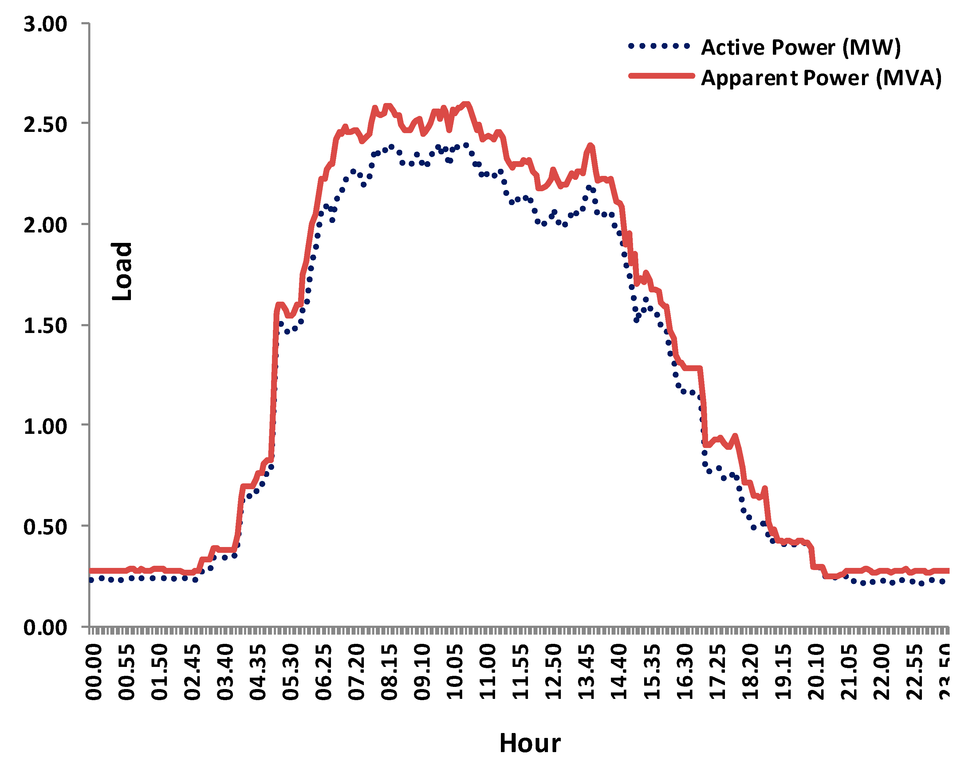
2. Examination of the Studied Real Case Study in Egypt

Although Egypt is rich in various renewable energy sources, these sources have not been optimally exploited yet [29]. Most of the generated electricity in Egypt is thermally produced from either gas, steam or combined cycle. Another source of electricity in Egypt is hydroelectric power derived by exploiting the energy of falling water through the river Nile dams. Figure 1 shows the renewable energy contribution compared to other electricity sources in the Egyptian electricity market in the fiscal year 2018–2019. The percentage of the installed capacity of renewable resources to the total electrical installed capacity in Egypt does not exceed 3.8%. The percentage of generated renewable energy to the total generated energy in Egypt also does not exceed 2.3%.

The strategy of the Egyptian electricity sector represented by the Electricity Holding Company (EEHC) aims to increase the contribution of renewable energy in Egypt to 42% by 2035. The EEHC has modified its policies to encourage private investments in renewable power generation projects. This explains the recently remarked relative increase in the installed capacity of renewable power sources. According to the recently published report of the EEHC, the contribution of renewable power sources increased during the last year from 2% to 3.8% of the total installed capacity. Regarding the actual generated energy, renewable energy increased during the last year from 1.46% to 2.3% of the total generated energy.

The New Valley region in the western desert of Upper Egypt is one of the promising regions on which development strategies are based according to Egypt’s Vision 2030. This region is well-known for its richness in various types of mineral wealth, soil fertility and the availability of groundwater. The recently published solar atlas of Egypt indicates that this region has another treasure. Figure 2 illustrates the yearly sum of global solar radiation over New Valley as compared to other Egyptian regions. The average yearly solar radiation over New Valley ranges between 2800 and 3200 kWh/m² according to the average values during the last 20 years. The daily duration of sunshine fluctuates between 9 and 11 h [29]. This climate gives New Valley the priority for investment in renewable energy projects.

Despite the efforts made by the EEHC to supply that region with electrical energy, the long distance between load demands and the existing unified national grid affects the power quality and makes connecting these loads to the unified national grid an uneconomic process. Therefore, some loads (around 38.5 MW) are still not connected to the unified national grid. These isolated loads include 32.5 MW powered by diesel generators while only 6 MW are supplied by solar energy.

Two far demand areas (Arbien and Max) located in the New Valley region were selected as a case study. The two areas are electrically fed by the same DN. Figure 3 illustrates the location of this Upper Egypt distribution network (UEDN) compared to the path of the Egyptian unified electrical grid. The single-line diagram of the existing network that supplies these areas with electrical energy is shown in Figure 4. The selected areas are supplied from the Kharja substation through the transformer 5T of capacity 25 MVA with a transformation ratio of 66/22 kV. The Kharja substation is connected to the extra-high-voltage grid through the Abo Tartor substation 220/66 kV by two circuits. Each circuit is constructed by an overhead line of aluminum conductors steel reinforced (ACSR) with a cross-sectional area of 380/50 mm² and 48 km in length. A detailed description of the studied network and its load distribution is given in Section 5.2.

3. Modeling of DN Components

The realization of any power-flow algorithm requires first an establishment of a model for each component of the DN. A component model is mainly built with physical and electrical specifications given in the manufacturing catalogs. Figure 5 shows a simplified single-line diagram and an electric equivalent of an ADN portion containing DG, distribution transformer, SCB and AVR connected to node k. The following subsections describe the modeling of each element in this segment [30].

3.1. Modeling of Distribution Line

The typical π-model has been generally used to implement the modeling of a distribution line segment connecting two nodes. The series impedance matrix $Z$ of any three-phase line segment is represented as [16]:

$$Z=l·\left(\begin{array}{ccc}{z}_{11}& z_{12}& z_{13}\\ z_{21}& z_{22}& z_{23}\\ z_{31}& z_{32}& z_{33}\end{array}\right)$$

(1)

where $l$ is the segment length. Element $z_{ii}$ along the diagonal of the series impedance matrix is the self-impedance of conductor $i$ per unit length. Element $z_{ij}$ along the off-diagonal is the mutual impedance between conductors $i$ and $j$ per unit length. Equations (2) and (3) use the modified Carson’s equations [16] to represent the self and mutual impedances, respectively.

$$z_{ii}=r_d+R_{ref}\left(1+\alpha \left(T-T_{ref}\right)\right)+j\left[\left(2\pi f\right)\left(0.2\times {10}^{-3}\right)\ln \left(\frac{D_e}{GMR}\right)\right]$$

(2)

$$z_{ij}=r_d+j\left[\left(2\pi f\right)\left(0.2\times {10}^{-3}\right)\ln \left(\frac{D_e}{GMD}\right)\right]$$

(3)

where $r_d$, $\alpha$, $T$ and $f$ are the resistance of dirt in $\Omega /km$, the temperature coefficient of conductor material, the operating temperature in $℃$ and the system frequency in Hertz, respectively. The reference resistance $R_{ref}$ in $\Omega /km$ of conductor $i$ is given by the manufacturer at a reference temperature $T_{ref}=20 ℃$. The distances $D_e$, $GMR$ and $GMD$ in meters are, respectively, the distance from conductor $i$ to dirt, the geometric mean radius of conductor $i$ and the geometric mean distance between the three conductors. Although the shunt admittance at the distribution voltage level is small enough to be neglected, the model has the flexibility to include that effect.

3.2. Modeling of Transformer Losses

A three-phase distribution transformer converts the consumed or generated power at the low-voltage network to the medium voltage network, along with the real and reactive power dissipated by that transformer. The power dissipated inside the distribution transformer shown in Figure 5 is given by [31,32,33]:

$$S_{Tk}=\left(P_o{\left(\frac{V_k}{V_r}\right)}^2+P_c{\beta }^2{\left(\frac{V_r}{V_k}\right)}^2\right)+j\left(I_o{S}_r{\left(\frac{V_k}{V_r}\right)}^2+U_x{S}_r{\beta }^2{\left(\frac{V_r}{V_k}\right)}^2\right)$$

(4)

where $S_{Tk}$ is the apparent power that dissipated inside the transformer, $V_r$ is the rated voltage, and $V_k$ is the node voltage. $S_r$ and $\beta$ are the transformer-rated power and the transformer loading percentage, respectively. $P_o$, $P_c$ and $I_o$ are the no-load losses, full-load losses and percentage of no-load current, respectively. The parameter $U_x$ in Equation (4) represents the reactive part of the percentage short-circuit voltage, which can be expressed as [31,32,33]:

$$U_x=\sqrt{U_s{}^2-{\left(\frac{100P_c}{S_r}\right)}^2}$$

(5)

where $U_s$ is the percentage of short-circuit voltage given by the transformer manufacturer.

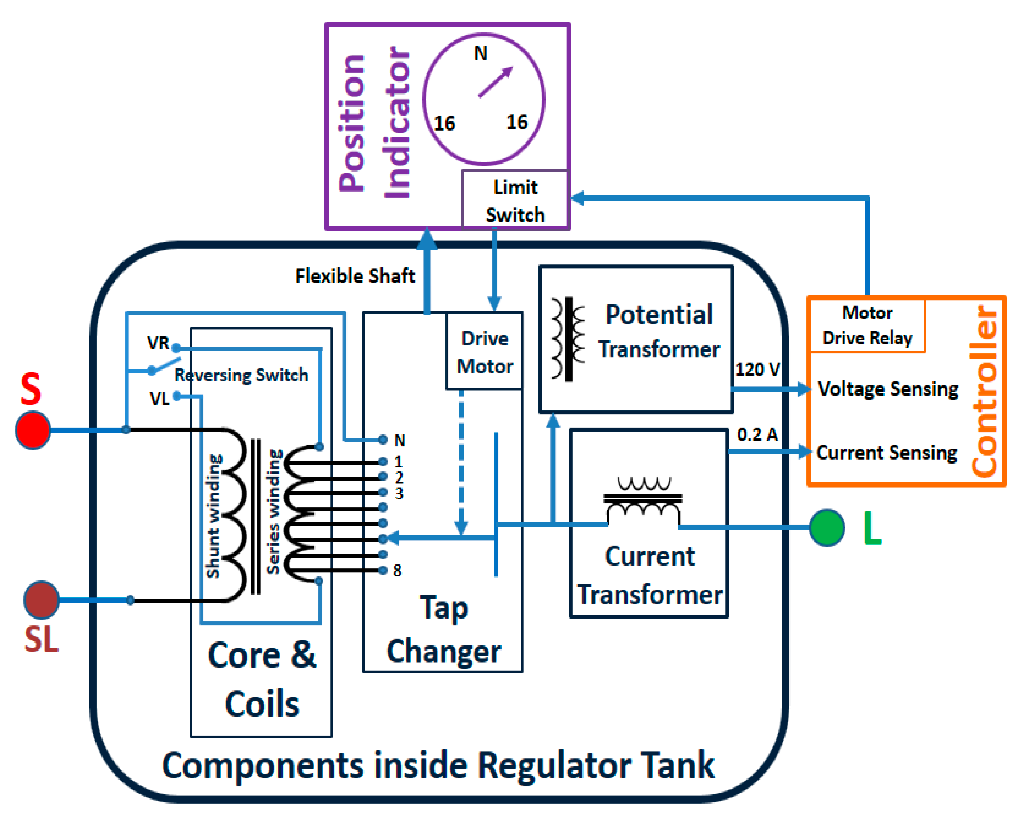
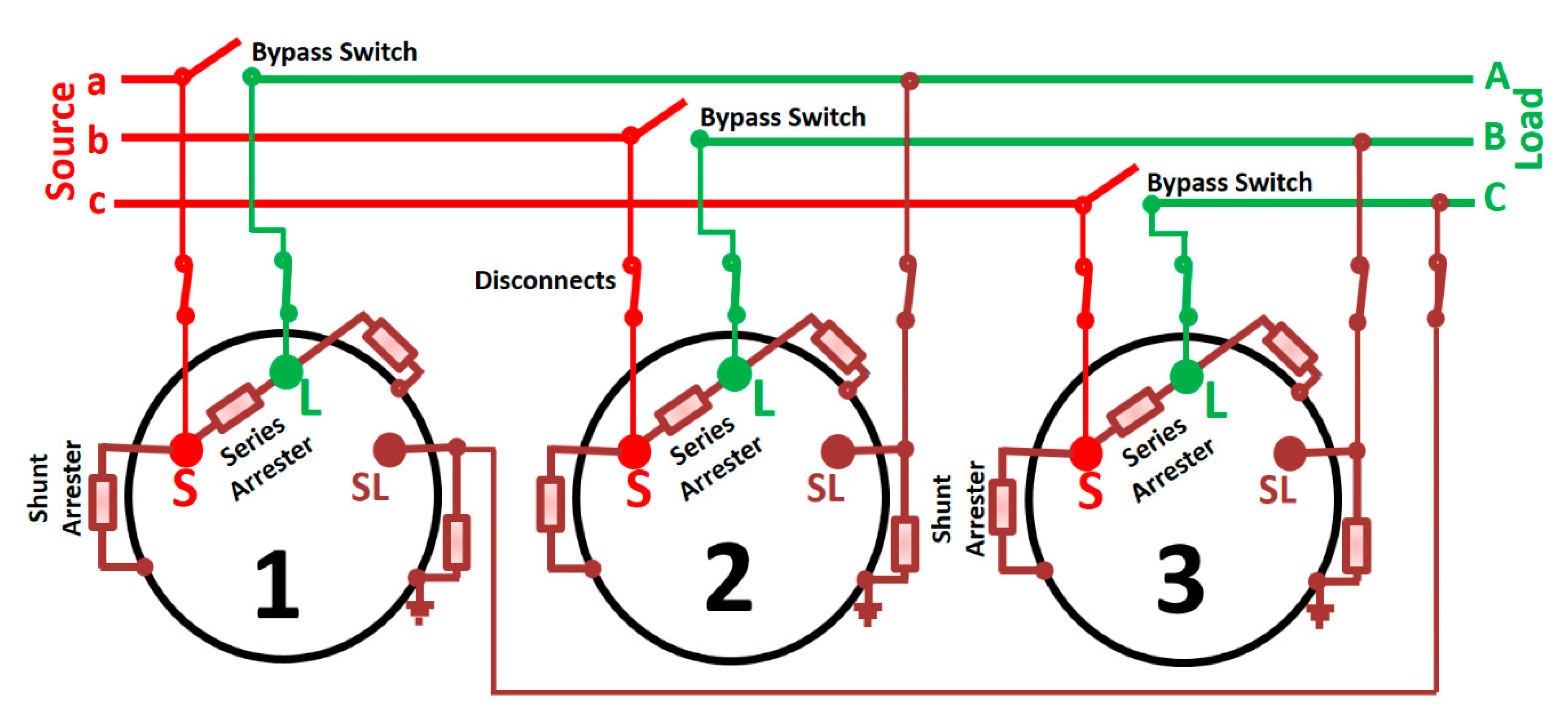
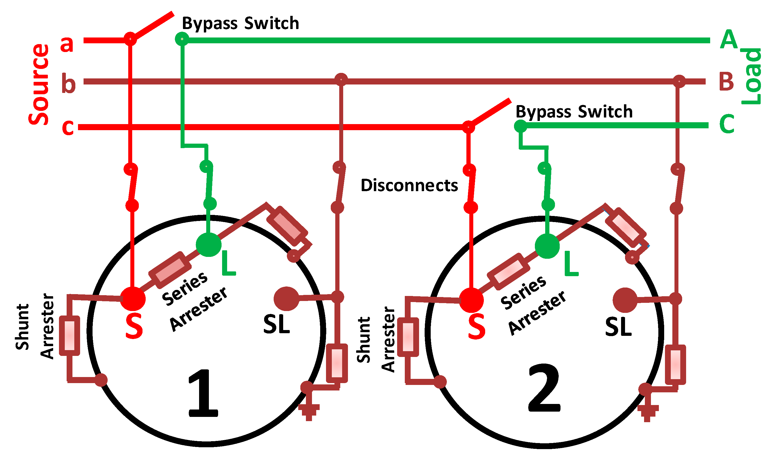
3.3. Modeling of AVR

AVR is a normal auto-transformer equipped with an automatic tap-changing mechanism [34,35,36,37,38,39]. Standard AVR provides ±10% voltage regulation in 32 steps of approximately 5/8% each. The tap of maximum raise position is 16R, while 16L is the tap of minimum lower position. The AVR has an automatic tap-changer able to switch from 16R to 16L and vice versa in less than 10 s.

According to the IEEE Std. C57.15-2009 (IEC60076-21:2011) standard [36], AVR is manufactured in one of two types: ANSI type-A and ANSI type-B. Figure 6 shows the overall functional diagram of a single-phase type-A regulator unit. Commonly, distribution utilities prefer to use three individual single-phase regulators rather than a single compact three-phase unit because the practical unbalance in voltage requires controlling each phase individually. The presence of more than one winding inside the same tank raises the winding and oil temperature, which means more losses. Additionally, the size of a single-phase AVR unit is much smaller as compared to a compact three-phase unit; this facilitates the processes of transportation, installation and maintenance. Moreover, in case of damage or fault in a single-phase AVR unit, the remaining two units can be reconnected as an open-delta configuration to continue voltage regulation during the period of repairing or replacing the damaged unit.

Since the common configuration of a primary DN is delta, single-phase AVR units are typically grouped in one of two connections [16]: closed-delta or open-delta. Figure 7 shows the closed-delta connection where three single-phase units are required to provide up to 15% voltage regulation. In an open-delta connection, only two units can be used to provide up to 10% voltage regulation as illustrated in Figure 8.

The relationship between the source voltage and current ($V_{Source}$ and $I_{Source}$) to the load voltage and current ($V_{Load}$ and $I_{Load}$) are governed by [16,37,38,39]:

• For Type-A Regulator:

  $$V_{Source}=\frac{1}{a_R}·V_{Load},I_{\begin{array}{c}Sou\\ 6rce\end{array}}=a_R·I_{Load}$$

  (6)

  where

  $$a_R=\{\begin{array}{c}1+N_R·Tap for raise taps\\ 1-N_R·Tap for lower taps\end{array}$$

  (7)
• For Type-B Regulator:

  $$V_{Source}=a_R·V_{Load},I_{Source}=\frac{1}{a_R}·I_{Load}$$

  (8)

  where

  $$a_R=\{\begin{array}{c}1-N_R·Tap for raise taps\\ 1+N_R·Tap for lower taps\end{array}$$

  (9)

In Equations (7) and (9), $N_R$ is the per unit regulation of single step ($N_R=0.00625$ for a step-type AVRs), and $Tap$ is the tap position of the current step.

3.4. Modeling of DG Unit

DG is a relatively small power generator directly connected to the DN owned by the distribution system operator (DSO) or connected at the customer side beyond the point of common coupling. DG unit can be one of the following types [40]: (1) photo-voltaic system, (2) wind turbine, (3) fuel cell, (4) gas turbine, (5) internal combustion engine or (6) micro-turbine. Regarding their power production, DG units are classified into four types: (1) Type-I produces real power only; (2) Type-II produces reactive power only; (3) Type-III produces both real and reactive power; and (4) Type-IV produces real power but consumes reactive power.

Regarding their modeling, DG units can be connected to power systems by one of four models [40,41,42,43]: (1) constant power factor model connected as PQ-node; (2) constant voltage model connected as PV-node; (3) P model; or (4) PQV model. The commonly used model at the distribution level is the constant power factor model because the DG units have a small capacity, which is insufficient to affect the voltage at the point of connection.

In the case of the constant power factor model, the DG unit is characterized by two main parameters. The first parameter is the real part of the generated power $P_{gk}$, and the second is the targeted power factor $P{F}_{gk}$. For the DG shown in Figure 5, the apparent power $S_{gk}$ generated at node $k$ can be expressed as [41]:

$$S_{gk}=P_{gk}\left(1+j\sqrt{P{F}_{gk}{}^{-2}-1}\right)$$

(10)

The power generated by a DG unit of that type is typically treated as a negative load injecting current to the network instead of drawing current from the network. Therefore, this point of connection can be considered as a PQ node.

3.5. Modeling of Shunt Capacitor Bank

Shunt capacitors are used in DNs to supply a part of the reactive power demands [44]. Therefore, the shunt capacitor bank (SCB) can be considered as a DG unit that generates only reactive power. The benefits of reactive power compensation in DNs using SCBs are power factor correction, voltage drop reduction, power loss reduction, system capacity release and power quality improvement.

SCB can be modeled as a delta-connected load of constant impedance. The effective reactive power of the SCB is proportional to the square value of voltage magnitude at the point of connection. For an SCB of rated reactive power $Q_{rk}$ at rated voltage $V_r$, its effective reactive power $Q_{Ck}$ when connected to node $k$ is calculated by [41]:

$$Q_{Ck}=Q_{rk}{\left|\frac{V_k}{V_r}\right|}^2$$

(11)

3.6. Load Models

The majority of the distribution power demands are domestic, industrial or commercial loads. The power consumed by these types of loads may vary according to voltage or frequency deviations from their rated values. As attention is focused here on the static analysis, only the voltage effects are considered, and the frequency effects may be neglected. Owing to their voltage dependence, distribution loads can be one or a mix of three models: (1) constant power (CP) model, in which the power consumed by the load does not depend on voltage changes; (2) constant current (CC) model, where the power consumed varies directly with voltage magnitudes; and (3) constant impedance (CI) model, in which the power consumed by the load varies directly with the square of voltage magnitudes. The power dependency of a certain load to voltage changes can be expressed in a general exponential form as [45]:

$$S_{Lk}=S_{rk}{\left(\frac{V_k}{V_r}\right)}^n$$

(12)

where $S_{Lk}$ is the consumed apparent power, $V_k$ is the node voltage, $S_{rk}$ is the rated apparent power of the load, $V_r$ is the rated voltage, and $n$ is the model exponent. By setting $n$ to 0, 1 or 2, the load type can be turned into CP, CC or CI, respectively [45].

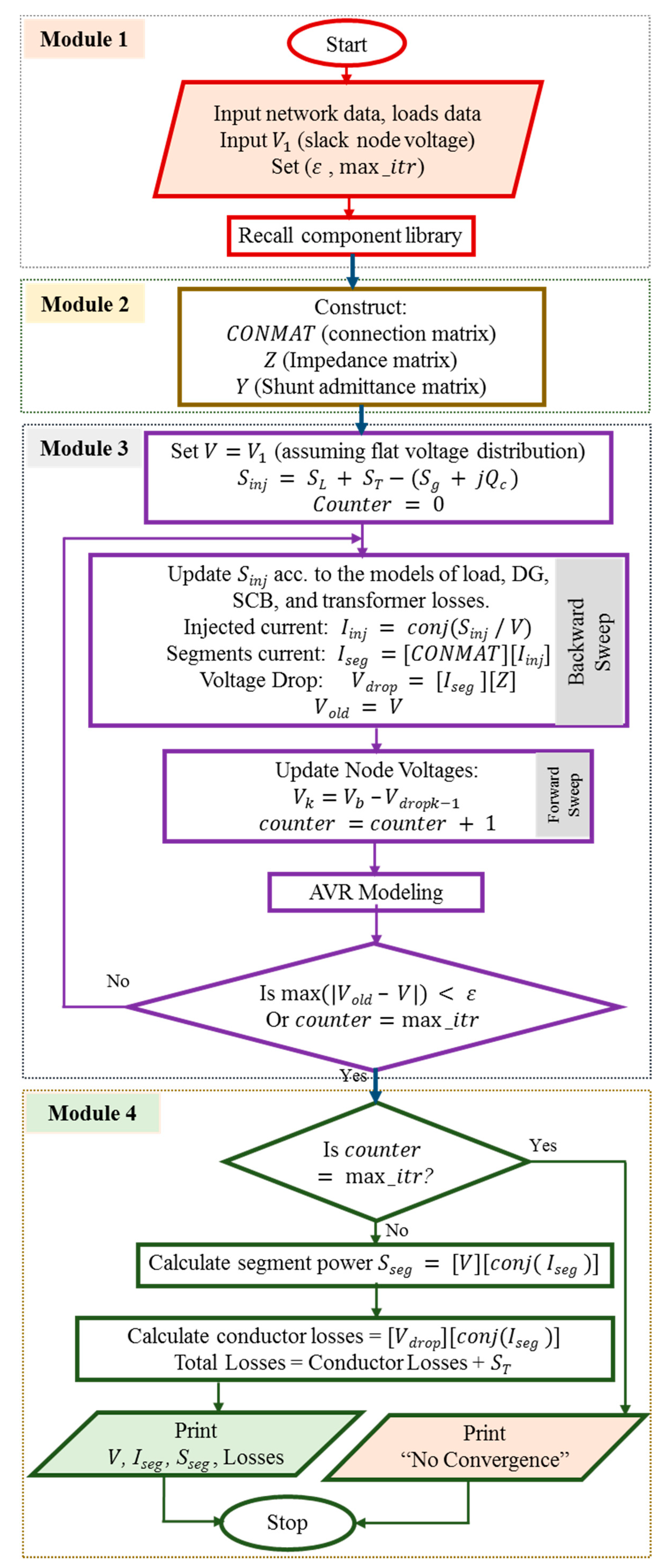
4. Proposed Power-Flow Algorithm

To describe the proposed power-flow algorithm, a general scheme of a three-phase distribution network is considered. The network is assumed to contain a total number of nodes $N_n$ and segments $N_s$. Typically, $N_s=N_n-1$ for radial DNs. The voltage $V_1$ at the slack node 1 (main substation) is generally taken as a base voltage. All other successive nodes are sequentially numbered. Figure 9 illustrates the program flow-chart. As shown, the algorithm consists of four modules: initialization, matrices construction, BFS iterations and losses calculations. The following subsections describe the algorithm sequence.

4.1. Module 1: Initialization

• Input the network data (specifications and locations of the network components).
• Input the loads data (locations, consumptions and types of all load points).
• Select the solution accuracy ($\epsilon$) and the maximum number of iterations ($max\_itr$).
• Recall the required parameters related to network components from the database library.

4.2. Module 2: Matrices Construction

• Construct the connection matrix ($CONMAT$) [30], the series impedance matrix ($Z$) and the shunt admittance matrix ($Y$).

4.3. Module 3: BFS Iterations

• Calculate the power injected at each node $S_{inj}$ assuming a flat voltage profile. $S_{inj}$ is the resultant of the load apparent power $S_L$ (Equation (12)), the transformer dissipated power $S_T$ (Equation (4)), the apparent power generated by DG unit $S_g$ (Equation (10)) and the effective reactive power of capacitor bank $Q_C$ (Equation (11)) if any.
• Repeat the following BFS iterations:

4.3.1. Backward Sweep Calculations:

• Correct $S_{inj}$ considering the load models, DG, SCB and transformer losses.
• Find the current injected to each node using: $I_{inj}={\left(S_{inj}/V\right)}^{*}$.
• Find the current flowed through each segment using: $I_{seg}=\left[CONMAT\right]\left[I_{inj}\right]$.
• Find the voltage drop across each segment using: $V_{drop}=\left[I_{seg}\right]\left[Z\right]$.
• Denote the calculated voltage distribution matrix $V$ of the current iteration as $V_{old}$.

4.3.2. Forward Sweep Calculations

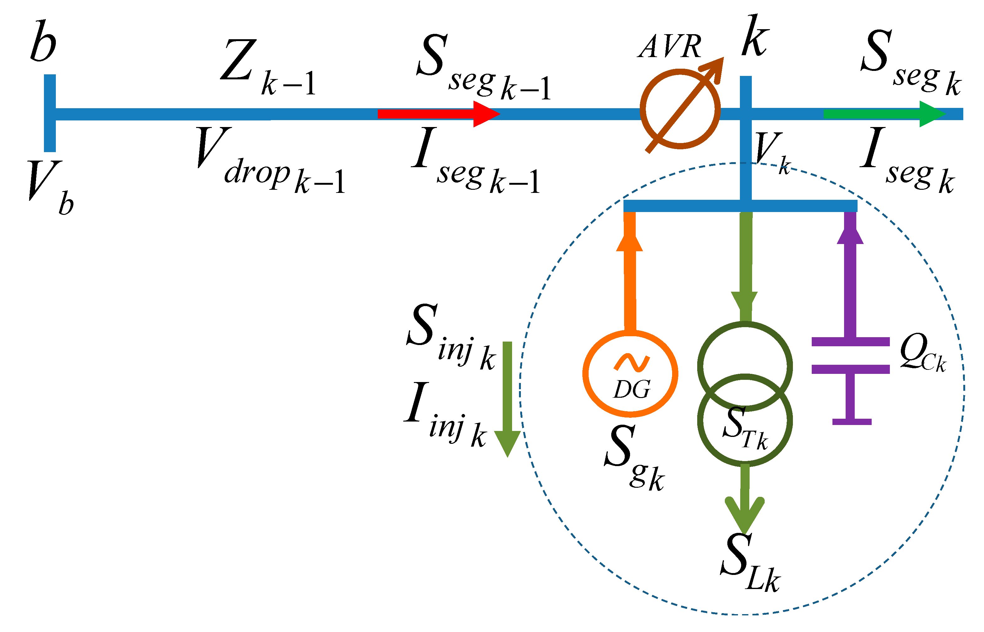
• Update the matrix $V$ according to the voltage drop $V_{drop}$ formerly determined in the backward sweep. Considering the voltage at any arbitrary node k ($V_k$ shown in Figure 5) is the voltage at its predecessor node b ($V_b$) minus the voltage drop across the segment connecting them ($V_{dropk-1}$).
• Recalculate both voltage and current matrices according to the AVR model.
• Update the loop counter.
• Terminate the loop if each element in the matrix ($V_{old} – V$) is less than the solution accuracy $\epsilon$, or the loop counter exceeds the maximum number of iterations ($max\_itr$).

4.4. Module 4: Losses Calculations

• Find the power flowed through each segment using: $S_{seg}=\left[V\right]{\left[I_{seg}\right]}^{*}$
• Find the conductor losses using $\left[V_{drop}\right]{\left[I_{seg}\right]}^{*}$
• Find the total losses by adding the conductor losses to the transformer losses.
• Print the outputs.

5. Simulation Results and Discussions

5.1. Case I: Unbalanced IEEE 37-Node Feeder

The unbalanced IEEE 37-node standard feeder is a PDN prepared to evaluate and benchmark distribution system models [46]. The proposed algorithm was applied first to this test feeder in its original PDN state. The algorithm was coded under MATLAB platform version R2016b. A laptop with an Intel (core i5 2.9 GHz) processing unit and 4 GB RAM was used to execute the algorithm. The execution time was 0.19 s.

Table 2. Voltage behavior of the ADN as compared to the passive distribution network (PDN) in case I.

Network		PDN			ADN
Line-to-line		A-to-B	B-to-C	C-to-A	A-to-B	B-to-C	C-to-A
Min. Voltage	(pu)	0.998	0.995	0.985	1.006	1.002	0.999
	at Node	741	722	741	741	722	741
Max. Voltage	(pu)	1.044	1.025	1.035	1.031	1.019	1.025
	at Node	701	701	701	701	701	701
Tap of AVR		7R	4R	-	5R	3R	-

presents the obtained results. Our results were found to be very close to the results published in [46]. By selecting a solution tolerance $\epsilon$ equals 10⁻⁶, the maximum founded deviation in the voltage magnitudes as compared to those given in [46] is less than 0.006%. The maximum deviation of the calculated power losses from those of [46] is less than 0.005%. This test asserted the effectiveness of the presented algorithm to analyze unbalanced DNs.

To convert this test system to an ADN, the network was divided into three zones. Each zone has a local area control center (LACC) to monitor and control the corresponding area. Each zone is supposed to have a constant power factor DG unit of type-III. The three DG units were assumed to have the same rated active power of 500 kW at 0.958 power factor for each. The DG units were located at nodes 720, 744 and 734. Figure 10 compares the line-to-line voltage profile along with the PDN nodes to that along with the ADN nodes. As shown, the conversion to ADN improves voltage unbalance. The shape of the voltage profile also appears to become more flattened in the case of the ADN.

Table 2 confirms the same results and clarifies how the conversion to ADN preserves the AVR. As concluded from

Table 3. Losses of the ADN as compared to the PDN in case I.

Network	PDN				ADN
Line	A	B	C	Total	A	B	C		Total
Losses (kW)	$26.669$	$13.804$	$20.087$	$60.560$	$8.118$	$4.076$		$5.918$	$18.112$

, the conversion to ADN greatly reduces the overall network loss to become less than 30% of its previous PDN value.

5.2. Case II: Balanced UEDN Network

Figure 11 shows the single line diagram of a 22 kV PDN located at the western desert of Upper Egypt as explained in Section 2. This network is dedicated to supplying an agriculture load at a location far from the nearest power source by more than 100 km. The load consists of 39 electric pumps. Each pump raises water from a deep well to irrigate a farm. The maximum power demand of this area was insufficient to construct a new power station there. Therefore, the DSO was forced to extend that long PDN.

As shown in Figure 11, the UEDN has two groups of AVRs placed at node 4 and node 11. The two AVR groups have the technical data listed in

Table 4. Specifications and sittings of the AVR groups in the Upper Egypt distribution network (UEDN).

Location Node	ANSI Type	Rated Current (A)	Connection Type	Voltage Level Setting (V)
$\mathbf{4}$	$B$	$300$	$\mathrm{Closed} \mathrm{Delta}$	$120$
$\mathbf{11}$	$B$	$300$	$\mathrm{Closed} \mathrm{Delta}$	$115$

. Detailed network data and solution variables are listed in the Appendix A. The electrical loads of this network are symmetrical and identical. Each load point feeds a three-phase pump of 88 kVA at 0.9 power factor (PF). Each pump is supplied through a transformer of 20/0.4 kV transformation ratio and 300 kVA rated power. The transformer has a tap-changer to select between seven steps manually: two steps to reduce the output voltage, one step for a neutral position without any voltage regulation and four steps to raise the output voltage. The tap-changer is designed to achieve voltage ‎regulation in the output voltage equal to 2.5% of the input voltage. The average voltage ‎magnitude measured at node 1 (Kharja substation) during the ‎day-time equals 21.5 kV. During the night-time, the same average equals 22.5 kV. A power quality analyzer device (model HIOKI 3196) was used to measure and record different electrical parameters at node 12 that is about 103.3 km from the Kharja substation. All measurements were recorded for 72 ‎h with an interval of 5 min between successive records.‎ Figure 12 displays the load profile during 24 h measured at node 12. The displayed profile repeats daily.

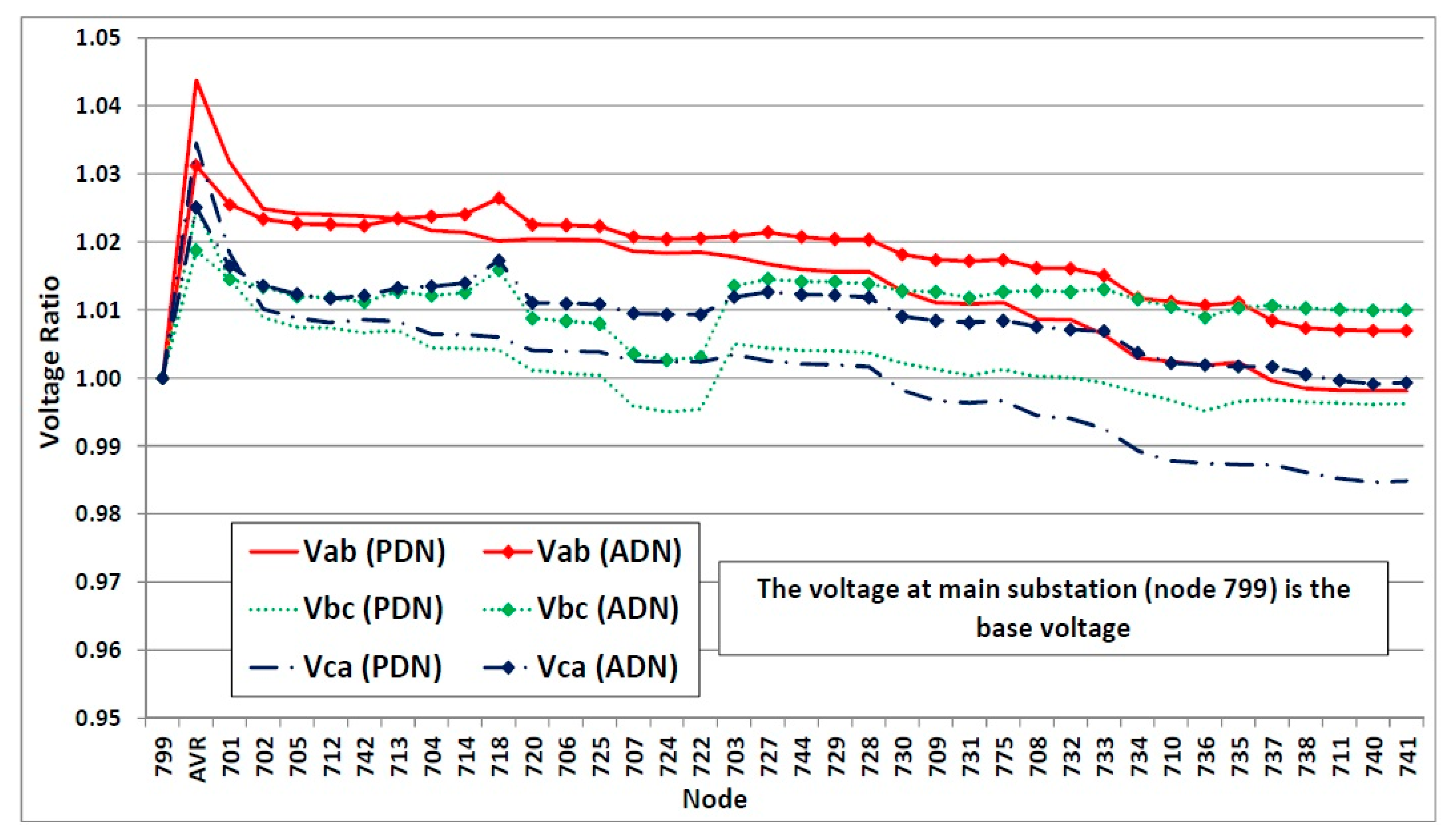
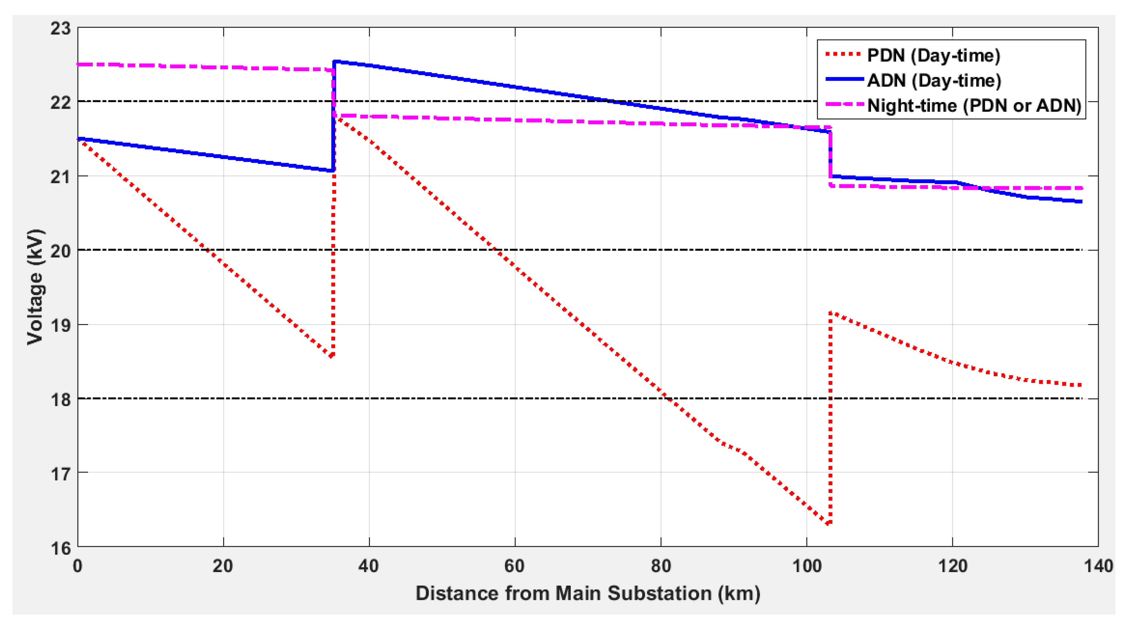
5.2.1. PDN Performance

The passive form of the UEDN is analyzed under two operating modes: the day-time mode and the night-time mode, as follows:

(a) Day-time Mode

During the day-time, irrigation pumps draw their maximum rated power. At that time, the voltage magnitude at the Kharja substation is 21.5 kV. The output results confirm that the two voltage regulators operate at tap 16R. However, some pumps suffer from the operation below their permissible voltage limit. Therefore, these loads draw currents more than their rated values. This operation condition leads to an increase in power losses and reduces the motor lifetime. The minimum voltage magnitude calculated at node 65 equals 18.2 kV. The percentage of voltage regulation equals 17.4%, which exceeds the allowable operating limits. The load at node 63 is found to operate in a critical condition. Its calculated voltage equals 364 V (9% below its rated value). The calculated power losses equal 1.337 MW, i.e., 29.74% of the total supplied real power are losses.

(b) Night-time Mode

During the night-time, loads vanish. The only flowed power is the losses resulted from unloaded transformers in-service. At that time, the voltage at the Kharja substation is 22.5 kV which is higher than its rated value. Therefore, the calculated results confirm that the voltage regulator located at node 4 operates at step 3L while the other regulator located at node 11 operates at step 4L. This operational status of the two AVR groups maintains the voltage magnitudes at essential safe values. The calculated power losses equal 23.6 kW, i.e., all the supplied real power are losses.

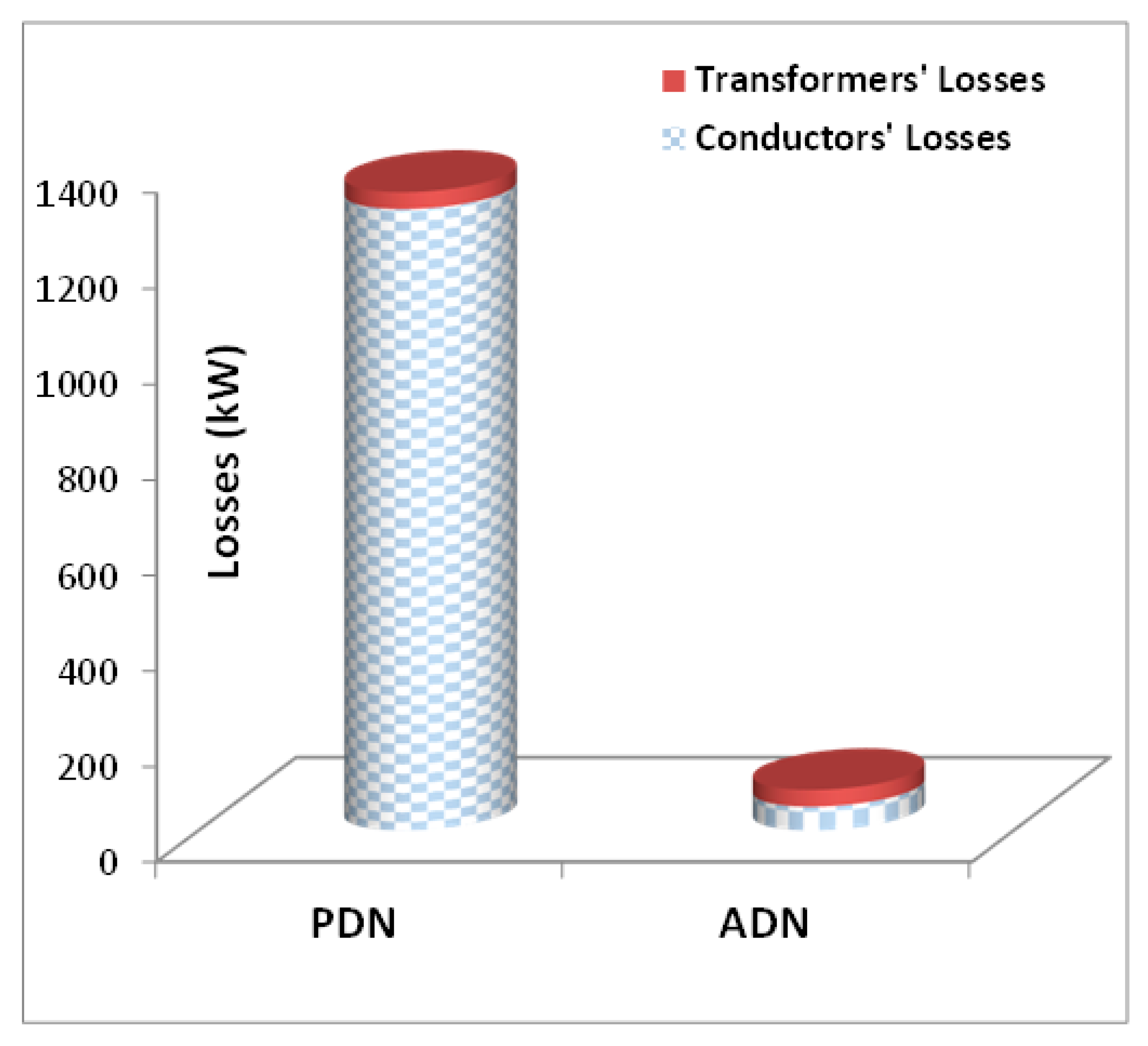
5.2.2. ADN Performance

To convert the passive UEDN to an ADN, the network was divided into three zones. (1) The first zone extends from node 1 to node 12 without load points; hence, there is no need to install DG units or LACCs in this zone. (2) The second zone is the Max area, which extends from node 13 to node 32 and contains 13 load points. Therefore, it is useful to install a DG unit and LACC at the zone center, node 21. (3) The third zone is the Arbien area, which extends from node 33 to node 65 and contains 26 load points. A suggested DG unit and LACC is required at the zone center, node 46. Rates and types of the suggested DG units are given in

Table 5. Required DG units to turn the passive UEDN into an ADN.

Location (at Node)	DG Type	Rated Active Power (kW)	Specified Power Factor
$\mathbf{21}$	$III, PQ$	$900$	$0.9$
$\mathbf{46}$	$III, PQ$	$1800$	$0.9$

.

Because of the following reasons, it is highly recommended to select the DG units as on-grid solar power stations:

• The daily repeated load profile, shown in Figure 12, is similar to the solar power irradiance curve [47]; load vanishes by sunset and returns by sunshine.
• The required lands to construct solar power stations are available.
• The annual mean insolation [48] is high at the case study location as explained in Section 2.

The conversion of the UEDN from a PDN to an ADN improves the overall behavior of the network as concluded from

Table 6. ADN performance as compared to the PDN in the UEDN under different loading conditions.

Network		PDN		ADN
Operation Mode		Day-Time (Full Load)	Night-Time (No Load)	Day-Time (Full Load)	Night-Time (No Load)
$Substation Voltage \left(kV\right)$		$21.5$	$22.5$	$21.5$	$22.5$
$Min. Load Voltage$	$Magnitude \left(kV\right)$	$18.17$	$20.83$	$20.65$	$20.83$
	$Location Node$	$65$	$65$	$65$	$65$
$Max. Load Voltage$	$Magnitude \left(kV\right)$	$19.14$	$20.86$	$20.99$	$20.86$
	$Location Node$	$15$	$15$	$18$	$15$
${Conductors}^{\prime } Losses$	kW	$1301.3$	$1.2$	$50.1$	$1.2$
	%	$28.95$	$4.97$	$1.55$	$4.97$
${Transformers}^{\prime } losses$	kW	$35.28$	$22.46$	$35.28$	$22.46$
	%	$0.79$	$95.03$	$1.10$	$95.03$
$Total Losses$	kW	$1336.7$	$23.65$	$85.33$	$23.65$
	%	$29.74$	$100$	$2.63$	$100$
$Tap Position of AVR at node 4$		$16\mathrm{R}$	$3\mathrm{L}$	$7\mathrm{R}$	$3\mathrm{L}$
$Tap Position of AVR at node 11$		$16\mathrm{R}$	$4\mathrm{L}$	$3\mathrm{L}$	$4\mathrm{L}$

. This improvement is noticed in the total losses reduction, the voltage correction and the convenient operation of AVR groups. Figure 13 confirms the reduction in the total network losses from 1.34 MW (29.74% of the total consumed power in the PDN) to 85.3 kW (2.63% of the total consumed power in the ADN). This reduction is mainly due to the great reduction in conductors’ losses while the transformers’ losses remain the same.

Figure 14 compares the voltage profile along the ADN length to that of the PDN during different operating modes. As shown, the ADN moves the operating voltage at load points from a near-critical limit (18 kV) to a safe operation state (21 kV). It is also clear that the ADN narrows the wide gap between day-time and night-time voltage profiles. Narrowing this gap removes the daily repeated thermal and electrical stresses on network insulations. Obviously, the ADN also decreases the daily-accumulated number of AVR steps. Therefore, the ADN leads to the convenient operation of AVR groups and extends the AVR lifetime.

The algorithm presented in this paper considers only one DG model—the constant power factor model. Modeling other DG types is planned to be covered in future work. In addition, our future work will include harmonic effects and sub-transient network states.

6. Conclusions

A new algorithm for power-flow calculations based on the BFS method was developed in this paper. Modeling of the commonly used medium voltage components including distribution line, AVR, DG unit and SCB was presented. Moreover, different load models and the power dissipated inside distribution transformers were also considered. The proposed models were integrated with the developed power-flow algorithm to form a comprehensive tool valid to simulate balanced or unbalanced ADNs. The proposed algorithm was tested on the standard IEEE 37-node feeder as an unbalanced network. The validation test confirmed the effectiveness of the presented algorithm to simulate unbalanced DNs. A remote PDN located in the western desert of Upper Egypt was highlighted as a practical balanced application of the proposed algorithm. The examined situation of the Egyptian electricity sector imposes the need to increase the future contribution of renewable energies. The passive 22 kV UEDN is suggested to be turned into an ADN by the installation of two DG units with two LACCs. The conversion of the UEDN from a PDN to an ADN improves the overall behavior of the network. The total network losses are reduced from 1.34 MW (29.74% of the total consumed power in the PDN) to 85.3 kW (2.63% of the total consumed power in the ADN). ADN moves the operating voltage at load points from a near-critical limit (18 kV) to a safe operation state (21 kV). ADN also narrows the wide gap between day-time and night-time voltage profiles which removes the daily repeated thermal and electrical stresses on network insulations. Moreover, ADN decreases the daily-accumulated number of AVR steps. This leads to the convenient operation of AVR groups and extends the AVR lifetime.

References

1. Dunstan, L.A. Machine computation of power network performance. Trans. Am. Inst. Electr. Eng. 1947, 66, 610–624. [Google Scholar] [CrossRef]
2. Dunstan, L.A. Digital load flow studies. Trans. Am. Inst. Electr. Eng. III-PAS 1954, 73, 825–832. [Google Scholar] [CrossRef]
3. Ward, J.; Hale, H. Digital computer solution of power flow problems. Trans. Am. Inst. Electr. Eng. III-PAS 1956, 75, 398–402. [Google Scholar] [CrossRef]
4. Tinney, W.F.; Hart, C.E. Power flow solution by Newton’s method. IEEE Trans. Power Appar. Syst. 1967, 86, 1449–1460. [Google Scholar] [CrossRef]
5. Stagg, G.W.; El-Abiad, A.H. Computer Methods in Power System Analysis; International Student, Ed.; McGraw Hill Kogakusha Ltd.: Tokyo, Japan; Auckland, New Zealand; Beirut, Liban, 1968. [Google Scholar]
6. Stott, B. Decoupled Newton load flow. IEEE Trans. Power Appar. Syst. 1972, 91, 1955–1959. [Google Scholar] [CrossRef]
7. Alsac, O.; Stott, B. Optimal load flow with steady-state security. IEEE Trans. Power Appar. Syst. 1974, 93, 745–751. [Google Scholar] [CrossRef] [Green Version]
8. Stott, B.; Alsac, O. Fast decoupled load flow. IEEE Trans. Power Appar. Syst. 1974, 93, 859–869. [Google Scholar] [CrossRef]
9. Kersting, W. A method to teach the design and operation of a distribution system. IEEE Trans. Power Appar. Syst. 1984, 103, 1945–1952. [Google Scholar] [CrossRef]
10. Cheng, C.S.; Shirmohammadi, D. A three-phase power flow method for real-time distribution system analysis. IEEE Trans. Power Syst. 1995, 10, 671–679. [Google Scholar] [CrossRef]
11. Teng, J.H. A direct approach for distribution system load flow solutions. IEEE Trans. Power Deliv. 2003, 18, 882–887. [Google Scholar] [CrossRef]
12. AlHajri, M.; El-Hawary, M. Exploiting the radial distribution structure in developing a fast and flexible radial power flow for unbalanced three-phase networks. IEEE Trans. Power Deliv. 2010, 25, 378–389. [Google Scholar] [CrossRef]
13. Hamouda, A.; Zehar, K. Improved algorithm for radial distribution networks load flow solution. Int. J. Electr. Power Energy Syst. 2011, 33, 508–514. [Google Scholar] [CrossRef]
14. Abul’Wafa, A.R. A network-topology-based load flow for radial distribution networks with composite and exponential load. Electr. Power Syst. Res. 2012, 91, 37–43. [Google Scholar] [CrossRef]
15. Shakarami, M.; Beiranvand, H.; Beiranvand, A.; Sharifipour, E. A recursive power flow method for radial distribution networks: Analysis, solvability and convergence. Int. J. Electr. Power Energy Syst. 2017, 86, 71–80. [Google Scholar] [CrossRef]
16. Kersting, W.H. Distribution System Modeling and Analysis, 4th ed.; CRC Press Taylor & Francis Group: Boca Raton, FL, USA, 2017; ISBN 978-1-3151-20782. [Google Scholar]
17. Jayamohan, M.; Drisya, K.; Bindumol, E.; Babu, C. Improved BFSA for computation of power loss and voltage profile in radial distribution system. In Proceedings of the IEEE International Conference on Electrical, Electronics, and Optimization Techniques ICEEOT, Tamil Nadu, India, 3–5 March 2016; pp. 3247–3250. [Google Scholar] [CrossRef]
18. Alinjak, T.; Pavić, I.; Stojkov, M. Improvement of backward/forward sweep power flow method by using modified breadth-first search strategy. IET Gener. Transm. Distrib. 2017, 11, 102–109. [Google Scholar] [CrossRef]
19. Hameed, F.; Al-Hosani, M.; Zeineldin, H.H. A Modified Backward/Forward Sweep Load Flow Method for Islanded Radial Microgrids. IEEE Trans. Smart Grid 2017. [Google Scholar] [CrossRef]
20. Theo, W.L.; Lim, J.S.; Ho, W.S.; Hashim, H.; Lee, C.T. Review of distributed generation (DG) system planning and optimisation techniques: Comparison of numerical and mathematical modelling methods. Renew. Sustain. Energy Rev. 2017, 67, 531–573. [Google Scholar] [CrossRef]
21. Salman, S.; Tan, S. Investigation into protection of active distribution network with high penetration of embedded generation using radial and ring operation mode. In Proceedings of the IEEE International Universities Power Engineering Conference UPEC, Northumbria University, Newcastle, UK, 6–8 September 2006. [Google Scholar] [CrossRef]
22. D’adamo, C.; Abbey, C.; Baitch, A. Development and operation of active distribution networks: Results of CIGRE C6.11 working group. In Proceedings of the International Conference and Exhibition on Electricity Distribution CIRED, Frankfurt, Germany, 6–9 June 2011. Paper 0311. [Google Scholar]
23. Yu, W.; Liu, D.; Huang, Y.; Abbey, C. Operation optimization based on the power supply and storage capacity of an active distribution network. Energies 2013, 6, 6423–6438. [Google Scholar] [CrossRef] [Green Version]
24. Pilo, F.; Jupe, S.; Silvestro, F.; El Bakari, K.; Abbey, C.; Celli, G.; Taylor, J.; Baitch, A.; Carter-Brown, C. Planning and optimisation of active distribution systems-An overview of CIGRE Working Group C6.19 activities. In Proceedings of the CIRED Workshop, Lisbon, Portugal, 29–30 May 2012. [Google Scholar] [CrossRef]
25. Mohammed, N.; Ciobotaru, M.; Town, G. Online parametric estimation of grid impedance under unbalanced grid conditions. Energies 2019, 12, 4752. [Google Scholar] [CrossRef] [Green Version]
26. Hoffmann, N.; Fuchs, F.W. Minimal invasive equivalent grid impedance estimation in inductive–resistive power networks using extended Kalman filter. IEEE Trans. Power Electron. 2013, 29, 631–641. [Google Scholar] [CrossRef]
27. Mohammed, N.; Ciobotaru, M.; Town, G. Fundamental grid impedance estimation using grid-connected inverters: A comparison of two frequency-based estimation techniques. IET Power Electron. 2020, 13, 2730–2741. [Google Scholar] [CrossRef]
28. Xiang, Y.; Liu, J.; Li, F.; Liu, Y.; Liu, Y.; Xu, R.; Su, Y.; Ding, L. Optimal active distribution network planning: A review. Electr. Power Compon. Syst. 2016, 44, 1075–1094. [Google Scholar] [CrossRef]
29. Sultan, H.M.; Diab, A.A.Z.; Kuznetsov, O.N.; Ali, Z.M.; Abdalla, O. Evaluation of the Impact of High Penetration Levels of PV Power Plants on the Capacity, Frequency and Voltage Stability of Egypt’s Unified Grid. Energies 2019, 12, 552. [Google Scholar] [CrossRef] [Green Version]
30. Radwan, A.A.; Foda, M.O.; Elsayed, A.M.; Mohamed, Y.S. Modeling and Reconfiguration of Middle Egypt Distribution Network. In Proceedings of the 19th IEEE International Middle East Power Systems Conference MEPCON, Cairo, Egypt, 19–21 December 2017. [Google Scholar] [CrossRef]
31. Wu, P.; Gu, J.; Qun, X.; Tao, Y. Distribution power flow calculation based on the load monitoring system. In Proceedings of the IEEE China International Conference on Electricity Distribution CICED, Shanghai, China, 5–6 September 2012. [Google Scholar] [CrossRef]
32. Wu, A.; Ni, B. Line Loss Analysis and Calculation of Electric Power Systems; John Wiley& Sons Singapore Pte Ltd.: Singapore, 2016; ISBN 978-1-1188-6727-3. [Google Scholar]
33. Huang, J.; Liu, M.; Zhang, J.; Dong, W.; Chen, Z. Analysis and field test on reactive capability of photovoltaic power plants based on clusters of inverters. J. Mod. Power Syst. Clean Energy 2017, 5, 283–289. [Google Scholar] [CrossRef] [Green Version]
34. Hill, L. Step type feeder voltage regulators. Trans. Am. Inst. Electr. Eng. 1935, 54, 154–158. [Google Scholar] [CrossRef]
35. Bishop, M.; Foster, J.D.; Down, D.A. The application of single-phase voltage regulators on three-phase distribution systems. In Proceedings of the IEEE Rural Electric Power Conference, Colorado Springs, CO, USA, 24–26 April 1994. [Google Scholar] [CrossRef]
36. International Electrotechnical Commission. IEC Standard 60076-21, Power Transformers—Part 21: Standard Requirements, Terminology, and Test Code for Step-Voltage Regulators; International Electrotechnical Commission: Geneva, Switzerland, 2011. [Google Scholar]
37. Kersting, W.H. The modeling and application of step voltage regulators. In Proceedings of the IEEE Power Systems Conference and Exposition PSCE, Seattle, WA, USA, 15–18 March 2009. [Google Scholar] [CrossRef]
38. Yan, R.; Li, Y.; Saha, T.; Wang, L.; Hossain, M. Modelling and Analysis of Open-Delta Step Voltage Regulators for Unbalanced Distribution Network with Photovoltaic Power Generation. IEEE Trans. Smart Grid 2016, 9, 2224–2234. [Google Scholar] [CrossRef] [Green Version]
39. González-Morán, C.; Arboleya, P.; Mojumdar, R.R.; Mohamed, B. 4-Node Test Feeder with Step Voltage Regulators. Int. J. Electr. Power Energy Syst. 2018, 94, 245–255. [Google Scholar] [CrossRef] [Green Version]
40. Moghaddas-Tafreshi, S.; Mashhour, E. Distributed generation modeling for power flow studies and a three-phase unbalanced power flow solution for radial distribution systems considering distributed generation. Electr. Power Syst. Res. 2009, 79, 680–686. [Google Scholar] [CrossRef]
41. Teng, J.-H. Modelling distributed generations in three-phase distribution load flow. IET Gener. Transm. Distrib. 2008, 2, 330–340. [Google Scholar] [CrossRef]
42. Elsaiah, S.; Benidris, M.; Mitra, J. Analytical approach for placement and sizing of distributed generation on distribution systems. IET Gener. Transm. Distrib. 2014, 8, 1039–1049. [Google Scholar] [CrossRef] [Green Version]
43. Tah, A.; Das, D. Novel analytical method for the placement and sizing of distributed generation unit on distribution networks with and without considering P and PQV buses. Int. J. Electr. Power Energy Syst. 2016, 78, 401–413. [Google Scholar] [CrossRef]
44. Baran, M.E.; Wu, F.F. Optimal capacitor placement on radial distribution systems. IEEE Trans. Power Deliv. 1989, 4, 725–734. [Google Scholar] [CrossRef]
45. Jagtap, K.M.; Khatod, D.K. Loss allocation in radial distribution networks with various distributed generation and load models. Int. J. Electr. Power Energy Syst. 2016, 75, 173–186. [Google Scholar] [CrossRef]
46. Kersting, W.H. Radial distribution test feeders. In Proceedings of the IEEE Power Engineering Society Winter Meeting, Columbus, OH, USA, 28 January–1 February 2001; Volume 2, pp. 908–912. Available online: http://sites.ieee.org/pes-testfeeders/resources/ (accessed on 29 June 2019). [CrossRef]
47. Messenger, R.A.; Ventre, J. Photovoltaic Systems Engineering, 3rd ed.; CRC Press Taylor & Francis Group: Boca Raton, FL, USA, 2010; ISBN 978-1-4398-0293-9. [Google Scholar]
48. Lynn, P.A. Electricity from Sunlight: An Introduction to Photovoltaics; John Wiley & Sons: New York, NY, USA, 2011; ISBN 978-1-119-96503-9. [Google Scholar]
Figure 1. Egyptian electricity sources in the fiscal year 2018–2019.
Sustainability 12 08991 g001
Figure 2. The yearly sum of global solar radiation in Egypt.
Sustainability 12 08991 g002
Figure 3. Case study location compared to the Egyptian unified national grid. “TH. POWER ST.” is referred to thermal power stations, “HY. POWER ST.” is referred to Hydraulic Power Station and “SS” is referred to Substation.
Sustainability 12 08991 g003
Figure 4. Single-line diagram of the case-study supply system.
Sustainability 12 08991 g004
Figure 5. Electric equivalent of an active distribution network (ADN) segment. AVR: automatic voltage regulator; DG: distributed generation.
Sustainability 12 08991 g005
Figure 6. Overall functional diagram of the AVR.
Sustainability 12 08991 g006
Figure 7. Closed-delta connection of AVR units.
Sustainability 12 08991 g007
Figure 8. Open-delta connection of AVR units.
Sustainability 12 08991 g008
Figure 9. Flow-chart of the power-flow algorithm. SCB: shunt capacitor bank.
Sustainability 12 08991 g009
Figure 10. Voltage profile comparison between the ADN and PDN in case I.
Sustainability 12 08991 g010
Figure 11. Single-line diagram of the UEDN.
Sustainability 12 08991 g011
Figure 12. Daily load profile of the UEDN measured at node 12.
Sustainability 12 08991 g012
Figure 13. Losses reduction by converting the UEDN from a PDN to an ADN.
Sustainability 12 08991 g013
Figure 14. Voltage profile along the UEDN as an ADN compared to PDN under different loading conditions.
Sustainability 12 08991 g014