Individual Investors, Average Skewness, and Market Returns

Abstract

Understanding individual investors’ short-term behavior toward skewness is essential for the management and investment of corporate social responsibility because the skewness-seeking behavior of individual investors, which causes a bubble in the market, makes the market as a whole more vulnerable, and it is difficult for the market to be sustainable. In the Korean stock market, we investigated whether average skewness can predict future market returns at the market level and whether the mispricing is associated with demand for the skewness of individual noise traders. Measuring the demand for skewness by the proportion of trading money of individual investors, we found that average skewness negatively predicts future market excess return when the demand for skewness is strong. The result is robust to controlling for market variance as well as other predictors. Our finding indicates that the overall market is overpriced when individual investors excessively trade to seek huge returns in spite of a small probability.

1. Introduction

It is well-known that individual investors exhibit strong preferences for huge positive returns in spite of a very small probability of realization [1,2,3,4]. Evidence shows that they often buy stocks with high skewness or high volatility at expensive prices in order to entertain the likelihood of jackpot. Since traditional portfolio theories such as the capital asset pricing model (CAPM) [5,6] assume that all investors hold fully diversified portfolios to eliminate idiosyncratic risks such as volatility and skewness, individual investors’ behavior of seeking skewness has attracted much attention of academics. Indeed, a bunch of research provides evidence that most individuals hold only a few equities, and their portfolios are under-diversified with respect to idiosyncratic risks rather than well-diversified.

Such behavior of individual investors affects asset prices in a different way than traditional finance portfolio theories predict. For example, Barberis and Huang [2] provided an equilibrium model in which skewness can be priced. If investors have cumulative prospect utility, stocks with positive skewness are overpriced since investors are willing to pay more to take a chance of large gains. Jondeau et al. [7] went one step further and analyzed the skewness-return relation at the market level. Their model suggests that the cross-sectional average of idiosyncratic skewness predicts future market excess returns.

Motivated by these studies, we analyzed how the trading behavior of individual investors affects the relation between average skewness and market returns. Given that individual investors prefer buying positively skewed stocks, we hypothesized that the average skewness and market return relation will be more apparent during periods when the participation of individual investors is high in the stock market. Since investor type information is available in the Korean stock market, differently from the U.S. market, we measured the level of participation of individual investors in terms of trading volume ratio and identified high and low skewness demand periods. Then we examined if the level of skewness demand (or participation of individual investors) affects the predictability of average skewness for future market returns by running predictive regressions for each period.

Even though many studies have provided evidence that individuals do not hold well-diversified portfolios and skewness affects stock returns, papers that investigate the role of individual investors in the skewness and return relation at the market level are scarce. We attempted to fill this gap. While Jondeau et al. [7] showed that average skewness predicts subsequent market returns, we provided evidence that the relation depends on the degree to which individual investors are present in the market. Consistent with our expectation, the empirical result shows that when the market-wide demand for skewness is high, the relation is statistically and economically significant. In addition, during low skewness demand periods, we could not find any significant relation between average skewness and future market returns. This finding indicates that the under-diversification of individual investors plays an important role in the relation.

2. Literature Review and Hypothesis Development

2.1. Demand for Skewness and Corporate Social Responsibility

Before reviewing related papers and developing our hypothesis, this section explains why studying individual investors’ behavior is important for sustainable investments that consider environmental (E), social (S), and corporate governance (G) concerns. Most studies on corporate social responsibility (CSR) have focused on institutional investors because institutional investors are more pressured to be socially responsible for their investments by ethical standards and regulations. Thus, in the early stage of research on socially responsible investment (SRI), studies examined the performance of SRI mutual funds. For example, Statman and Glushkov [8] examined if socially responsible investors can earn higher returns relative to traditional investors. They found that there is no extra benefit because investing in stocks with high ESG scores earns higher returns, but the profit is offset by the underperformance of shunning investing in stocks with socially irresponsible characteristics such as tobacco, gambling, and weapons. Following the studies on SRI mutual fund performance, recent studies focused narrowly on institutional holdings instead of mutual funds. For example, Chen et al. [9] found that companies respond to the level of institutional holdings and change their CSR commitments.

Interestingly, Nofsinger et al. [10] provided empirical evidence that institutional preferences for ES indicators are related to stock skewness. They found that while institutions have a strong preference for shunning stocks with ES weakness, they are reluctant to put more weights on stocks with ES strength. This is because ES dimensions can reduce firms’ downside risk and increase positive skewness of stock returns. Hoepner et al. [11] also supported this by providing evidence that ESG engagements reduce the downside risk of a firm. In addition, Kim et al. [12] analyzed the relation between CSR and skewness of stock returns and found that CSR performance mitigates negative skewness of stock returns.

Despite the fact that individual investors’ demand for CSR seems to have driven significant growth of SRI mutual funds [10,13], few studies in CSR literature focused on individual investors, except Moss et al. [14]. In contrast to the conjecture of previous studies [10,13], Moss et al. [14] argued that retail investors do not pay attention to EGS disclosures. They collected data on retail investors using the Robin Hood application on their smartphones and found that those investors did not respond to press releases on EGS. Therefore, individual investors’ trading behavior is still questionable and worth to be investigated. If individual investors have a strong preference for positive skewness, companies will increase investment in CSR activities to mitigate downside risk and increase shareholders’ value.

2.2. Individual Investors and Skewness

This paper argues that when individual investors participate in the stock market more actively, the degree of under-diversification is higher, and average skewness is significantly negatively associated with expected market returns. We developed our hypothesis based on previous studies that have provided theoretical background and empirical evidence on individual investors’ preferences for skewness and the pricing of skewness. The following three streams of literature offer us the motivation for the hypothesis development.

First, many previous studies show evidence that investors are often reluctant to fully diversify their portfolios. The first empirical research about the degree of diversification of individuals was by Blume and Friend [15]. With two unique datasets including the 1971 Federal individual income tax returns and the Federal Reserve Board’s 1962 Survey of the Financial Characteristics of Consumers, they showed that individual portfolios consist of a very small number of assets which is insufficient to eliminate idiosyncratic risks. This fact suggests that households typically do not hold fully diversified portfolios. Using data from the Survey of Consumer Finances, Kelly [16] showed that the median stockholder holds only a single stock, and even high-income households own ten stocks. In addition to these seminal studies, Odean [17] and Polkovnichenko [18] also provided similar empirical evidence supporting the argument that individual portfolios are concentrated on several stocks. From a theoretical perspective, Guo and Wong [19] provided a stochastic dominance model to prove that the second-order stochastic dominance risk-lovers prefer holding some particular assets to diversifying in a portfolio. Thus, these studies suggest that individual investors prefer under-diversification rather than well-diversification, while portfolio theories based on Markowitz [20] imply that all investors hold fully diversified portfolios.

Second, extensive research indicates that investors have a preference for positive skewness and do not fully diversify their portfolios. From a theoretical perspective, Tversky and Kahneman [1] and Barberis and Huang [2] provided a model where an investor who has a cumulative prospect utility considers skewness in addition to the mean and variance of returns, and the skewness can be involved in investment decisions. Furthermore, recent studies argued that individual investors, who are typically less sophisticated and have smaller wealth, are more likely to prefer having an opportunity for a huge gain in spite of a tiny probability. For instance, Kumar [3] reported that relative to institutional investors, individual investors exhibit a stronger preference for lottery-like stocks having an asymmetric distribution of returns. Defining lottery characteristics as low price, high volatility, and high skewness, he provided evidence that individual investors put greater weights on stocks with lottery characteristics, while institutional investors allocate relatively less portfolio weight to such stocks.

Third, the relation between skewness and return has been examined theoretically and empirically in the literature. Kraus and Litzenberger [21] and Harvey and Siddique [22] developed models where systematic skewness (or co-skewness) is a determinant of asset prices. However, empirical evidence supporting their models are mixed and ambiguous. Meanwhile, Mitton and Vorkink [10] argued that under-diversification can cause a negative relation between idiosyncratic skewness and expected returns in equilibrium. If individual investors in the economy have different demands for skewness, then under-diversified portfolios maximize their expected utilities, and they are willing to sacrifice returns for positive skewness. As a result, idiosyncratic skewness rather than co-skewness can impact stock prices in equilibrium. While Mitton and Vorkink [10] viewed the pricing of idiosyncratic skewness at the stock level, Jondeau et al. [7] drew a similar implication at the market level. Jondeau et al. [7] documented that the average individual stock skewness should negatively predict future market excess returns if investors have a preference for skewness.

2.3. Hypothesis Development

Motivated by the previous studies, we assumed that the level of participation of individual investors measures the aggregate demand for skewness and used this proxy in the empirical investigation. Details will be provided in the following section. As the literature indicates, if individual investors have strong preferences for skewness and the skewness demand induces the negative relation between skewness and return, then the degree of participation of individual investors will be influential on the return and skewness relation. Thus, we hypothesized that at the market level, the negative relation between skewness and return is stronger during the period when individual investors more actively participate in the stock market or the aggregate demand for skewness is high. We examined this hypothesis at the market level. Thus, we expected that if month $t$ belongs to a high skewness demand month, average skewness in month $t$ negatively predicts the market excess return in month $t+1$. When the aggregate skewness demand is low or the participation rate of individual investors is low, the relation is expected to be weak or insignificant.

3. Data and Methodology

3.1. Main Variables

For the empirical analysis of the average skewness, we collected daily return data from FnGuide for all common stocks traded in two major boards of the Korea Exchange (KRX): the Korea Composite Stock Price Index (KOSPI) and the Korean Securities Dealers Automated Quotations (KOSDAQ). The sample covers the period from January 2000 to December 2018. In order to compute average skewness on a monthly basis, we followed Jondeau et al. [7]. First, we estimated the third moment of standardized daily returns for each stock in month $t$ as below:

$$S{K}_{i,t}={\displaystyle \sum }_{d=1}^K{\left(\frac{r_{i,d}}{{\sigma }_{i,t}}\right)}^3$$

(1)

where $r_{i,d}$ is the daily excess return of stock $i$ de-meaned by its time-series average in month $t$, $K$ is the number of trading days in month $t$, and ${\sigma }_{i,t}^2={\displaystyle \sum }_{d=1}^K{r}_{i,d}^2$. With the cross-section of $SK$ in month $t$, the monthly measure of the cross-sectional average skewness is measured by either equal-weight average skewness $CAS{K}_{ew,t}$ or value-weight average skewness $CAS{K}_{vw,t}$.

The moments of market excess returns were obtained as follows. We estimated the market variance in month $t$ by:

$$V_{m,t}={\displaystyle \sum }_{d=1}^K{r}_d^2+2{\displaystyle \sum }_{d=2}^K{r}_d{r}_{d-1}$$

(2)

where $r_d$ is date d market excess return de-meaned by its time-series average in month $t$, and $K$ is the number of trading days in month $t$. The second term of Equation (2) was employed to adjust the autocorrelation in daily returns. The market skewness $S{K}_m$ was estimated by the third moment of daily market excess returns in a similar manner with individual stock skewness. Market excess return is used in Equation (1).

3.2. Demand for Skewness

As discussed earlier, we assumed that relative to other sophisticated traders, individual investors have a stronger preference for skewness, and the level of aggregate demand for skewness can be measured by the trading concentration on individual investors. Following Kim and Park [23], we employed the trading proportion of individual investors as a proxy for the degree of skewness demand. The KRX provides information on what type of investors trades each stock; the investor type consists of foreign, institutional, and individual investors. We collected the amount of money traded by each investor type for each stock via DataGuide and aggregated the trading volumes to produce a market-wide demand. Specifically, the following equation computes the skewness demand ($\mathrm{SKD}$):

$$SK{D}_t=\frac{{\displaystyle \sum }BUY+SELL}{{\displaystyle \sum }Total Volume\times 2}$$

(3)

where BUY (SELL) is the amount bought (sold) by individual investors for each stock in month $t$, and Total Volume is the amount traded (bought or sold) by all types of investors in the same month. Note that the total amount bought by all investors is necessarily the same as that sold by all investors. Therefore, twice Total Volume measures the size of the total trades of a given stock. After aggregating the trading volumes across stocks, the aggregate trading volume of individual investors was divided by the aggregate trading volume of all investors. Thus, $SK{D}_t$ measures how much of the total trading is concentrated on individual investor trading at the market level. We assumed that this proxy can gauge the degree of skewness demand. That is, higher $SK{D}_t$ implies a stronger demand for skewness.

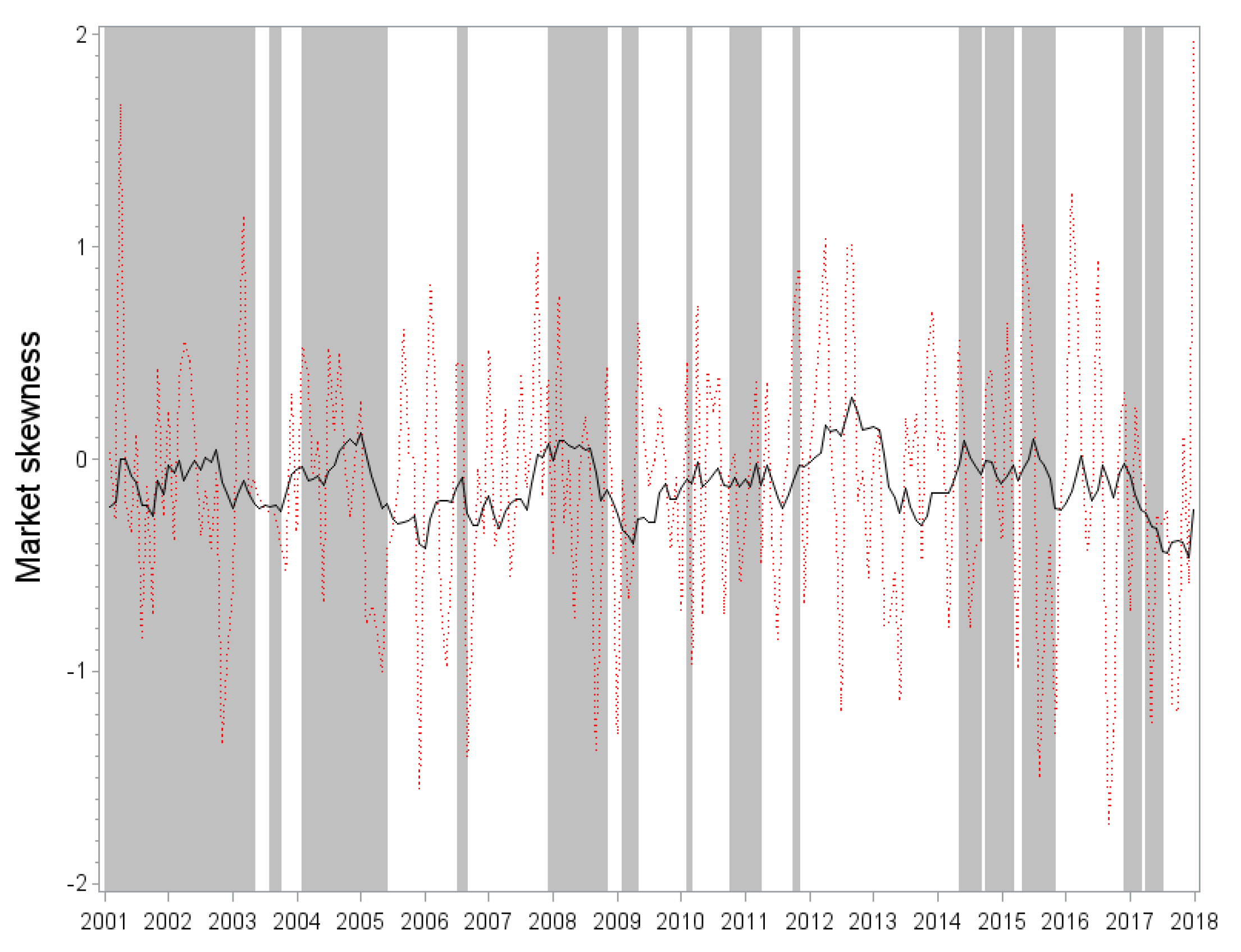
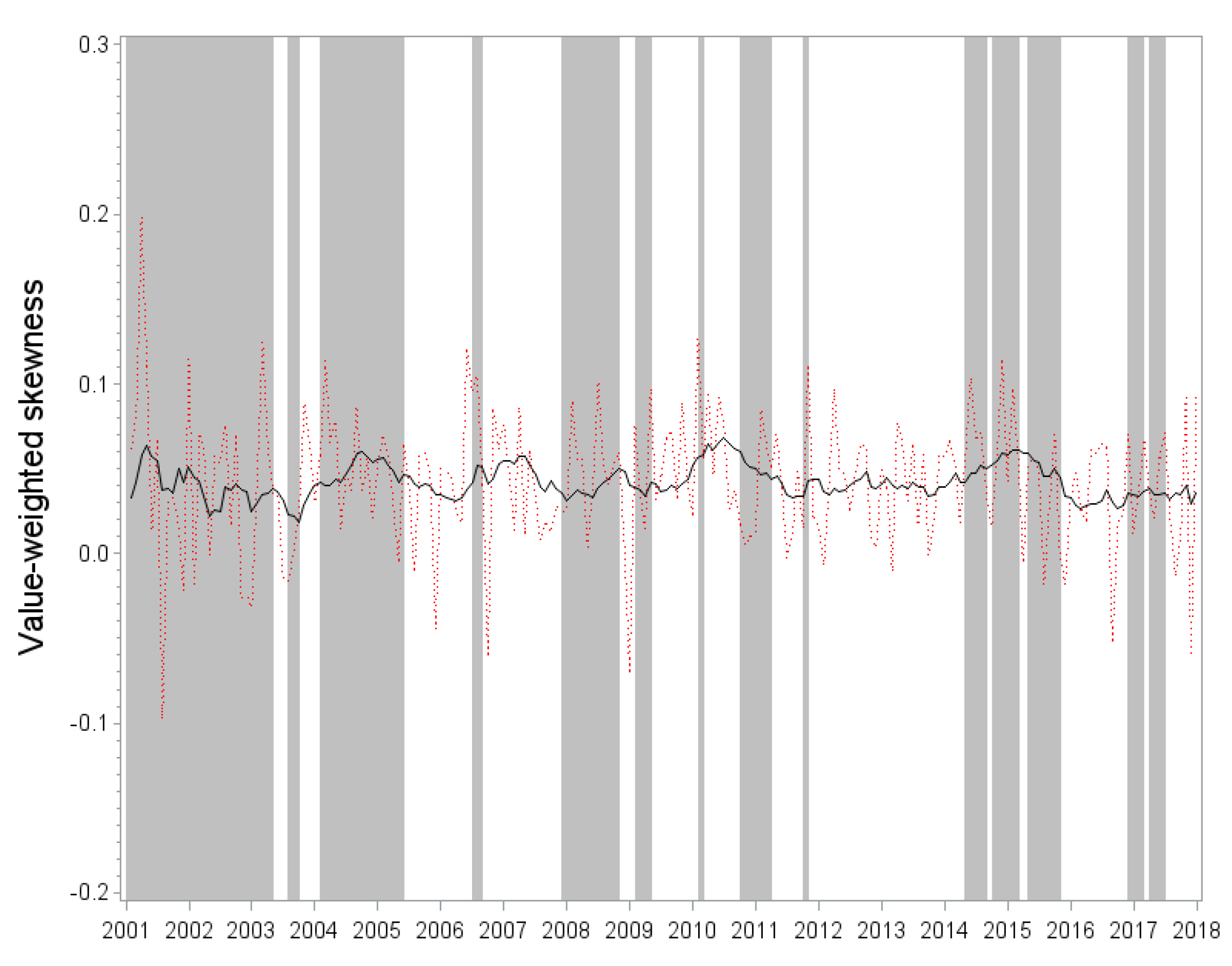
In the empirical analysis, we investigated the effect of SKD on the return and skewness relation depending on SKD regimes. We defined two SKD regimes as follows. Based on the median of historical $SK{D}_t$, we divided the months of the sample period into high (above median) and low (below median) skewness demand months. SKD ranged from 50% to 88% and had a median of 66% during the sample period, implying that 66% of trades were done by individual investors, on average. Out of 227 months in our 2001 to 2018 sample, 114 months fell into the high skewness demand (above an SKD of 66%) period, and the rest 113 months belonged to low skewness demand (below an SKD of 66%) period. In Figure 1 and Figure 2, high SKD periods are represented by shaded bars.

3.3. Descriptive Statistics

Summary statistics of the main variables are reported in

Table 1. Descriptive statistics of the main variables.

Panel A: Summary Statistics
Variable	Mean	Min	Median	Max	Std
$r_m$	0.004	−0.233	0.006	0.268	0.064
$V_m\times 100$	0.021	0.001	0.011	0.270	0.030
$S{K}_m$	−0.115	−1.720	−0.118	1.969	0.616
$CAS{k}_{vw}$	0.042	−0.156	0.046	0.198	0.042
$CAS{K}_{ew}$	0.061	−0.115	0.065	0.148	0.042
Panel B: Correlation
Variable	${\mathit{r}}_{\mathit{m},\mathit{t}+\mathit{1}}$	${\mathit{r}}_{\mathit{m}}$	${\mathit{V}}_{\mathit{m}}$	$\mathit{S}{\mathit{K}}_{\mathit{m}}$	$\mathit{C}\mathit{A}\mathit{S}{\mathit{K}}_{\mathit{v}\mathit{w}}$
$r_m$	0.054
$V_m$	−0.043	−0.377
$S{K}_m$	−0.017	0.047	−0.025
$CAS{K}_{vw}$	−0.099	0.377	−0.228	0.567
$CAS{K}_{ew}$	−0.057	0.506	−0.382	0.283	0.626
Panel C: Mean Values by Regimes
Regime	${\mathit{r}}_{\mathit{m}}$	${\mathit{V}}_{\mathit{m}}\times \mathbf{100}$	$\mathit{S}{\mathit{K}}_{\mathit{m}}$	$\mathit{C}\mathit{A}\mathit{S}{\mathit{k}}_{\mathit{v}\mathit{w}}$	$\mathit{C}\mathit{A}\mathit{S}{\mathit{K}}_{\mathit{e}\mathit{w}}$
Low SKD	−0.002	0.014	−0.061	0.038	0.057
High SKD	0.010	0.029	−0.169	0.046	0.065

. Panel A displays the mean, minimum, median, maximum, and standard deviation of the moments of market excess returns and the average skewness. Panel B shows the correlations among the variables, where $r_m$ is market excess return in month t, and $r_{m,t+1}$ is the market excess return in the next month. Panel C shows the mean values of each variable depending on the SKD regime.

We found that market skewness ($V_m$) and average skewness ($CAS{k}_{vw}$, $CAS{K}_{ew}$) display different behaviors over time. On average, market skewness is negative (−0.115), but value-weighted average skewness is positive (0.042). While market skewness fluctuates between −1.720 and 1.969, average skewness moves within a relatively narrow range. The standard deviation of each skewness also supports this. See also Figure 1 and Figure 2, where the time series of market skewness and value-weighted average skewness are plotted, respectively. In addition, the correlation between market skewness and average skewness is low. Specifically, market skewness is weakly associated with equal-weighted average skewness with a correlation coefficient of 0.283. Moreover, in Figure 1 and Figure 2 we confirm the fact that market skewness does not co-move with value-weighted average skewness. Around 2013 market skewness peaks, but average skewness stays at a moderate level.

Furthermore, the different patterns of the market and average skewness measures are distinctly observed depending on the SKD regimes in Panel C of Table 1 and Figure 1 and Figure 2. While market skewness is relatively higher in the low SKD period, average skewness is higher in the high SKD period. This fact indicates that the trading behavior of individual investors is closely associated with idiosyncratic skewness rather than systematic skewness. In addition, the proxy we suggest (SKD) does a good job of capturing the aggregate demand for skewness.

4. Empirical Results

4.1. Average Skewness and Future Market Returns

This section examines if average skewness predicts future market returns. To this end, we regress one-month ahead market excess returns, on a monthly basis, on the cross-sectional average of skewness values with the moments of contemporaneous market excess returns. Specifically, the following regression equation nests the testing models:

$$R_{m,t+1}=a+bCAS{K}_t+c{X}_t+{\epsilon }_{t+1}$$

(4)

where $R_{m,t}$ is the market excess return in month $t$ which is measured by the value-weighted average return of all stocks minus the commercial deposit (CD) 91-day rate. The major explanatory variable $CAS{K}_t$ is the cross-sectional average of the skewness of all stocks. In the analysis, we used value-weight $CAS{K}_{vw,t}$ or equal-weight averages $CAS{K}_{ew,t}$. A set of control variables $X_t$ includes the market skewness $SKE{W}_m$ as measured by the skewness of market excess returns in a given month, the market variance ${\mathrm{V}}_{\mathrm{m}}$ as measured by the variance of market excess returns in a given month, and the current market excess return.

Table 2. Predictive regressions of future market excess return on average skewness.

	M1	M2	M3	M4	M5	M6
Panel A: Value-weighted average skewness
Intercept	0.01 *	0.01 **	0.02 ***	0.01 **	0.02 **	0.02 ***
	(1.88)	(1.98)	(2.81)	(2.30)	(2.54)	(3.21)
$CAS{K}_{vw}$	−0.15*	−0.20 *	−0.23 **	−0.21 **	−0.29 **	−0.30 ***
	(−1.70)	(−1.89)	(−2.23)	(−2.13)	(−2.45)	(−2.65)
$SKE{W}_m$		0.01	0.01		0.01	0.01
		(0.89)	(1.10)		(1.33)	(1.40)
$V_m$			−0.16			−0.10
			(−1.07)			(−0.53)
$R_m$				0.11 *	0.12 **	0.11
				(1.83)	(1.99)	(1.31)
${\mathrm{R}}^2$	1.00%	1.20%	1.70%	1.90%	2.40%	2.60%
Panel B: Equal-weighted average skewness
Intercept	0.01	0.01	0.02 *	0.02 *	0.02	0.02 **
	(1.28)	(1.14)	(1.66)	(1.73)	(1.57)	(1.99)
$CAS{K}_{ew}$	−0.09	−0.09	−0.14	−0.17	−0.18	−0.20
	(−0.93)	(−0.82)	(−1.16)	(−1.53)	(−1.41)	(-1.63)
$SKE{W}_m$		0.00	0.00		0.00	0.00
		(0.01)	(0.11)		(0.19)	(0.25)
$V_m$			−0.16			−0.12
			(−0.93)			(−0.62)
$R_m$				0.11 *	0.11 *	0.10
				(1.80)	(1.77)	(1.23)
${\mathrm{R}}^2$	0.30%	0.30%	0.80%	1.20%	1.30%	1.50%
N	227	227	227	227	227	227

Note: The sample period covers 2001 to 2018. The 1%, 5%, and 10% statistical significance levels are denoted by ***, **, and *, respectively. Newey–West adjusted t-values are given in parentheses.

presents the result. Estimated coefficients are given with an indicator of the statistical significance. t-values in parentheses are adjusted by the Newey and West [24] procedure with 12 lags. Panels A and B show the results when value-weighted and equal-weighted average skewness measures were used, respectively.

In the value-weighted case given in Panel A, we see that average skewness ($CAS{K}_{vw}$) is negatively associated with future market returns. Although the statistical significance of the univariate regression (M1) is marginal, the other models with controls exhibit statistically significant and economically important results. Specifically, controlling for the contemporaneous market return, we see the more peculiar effect of average skewness on the future market return. The market skewness (${\mathrm{SKEW}}_{\mathrm{m}}$) and variance (${\mathrm{V}}_{\mathrm{m}}$) are positively and negatively related to future market returns, respectively. Although the coefficients are statistically insignificant and the sign of them is inconsistent with predictions of finance theories, the inclusion of the control variables makes the negative relation between average skewness and future market returns more significant.

We can approximately quantify the effect of average skewness as follows. M1 in Panel A of Table 2 indicates that an increase of average skewness by one standard deviation (0.042 as presented in Table 1) leads to a 0.6% decrease (= $-0.15\times 0.042$) in the market excess return in the next month. It is very interesting that this quantity is similar to that of the U.S. stock market, $-0.55\%$ according to Jondeau et al. [7]. Our result supports Jondeau et al. [7] by providing international market evidence in Korea.

The equal-weight case given in Panel B gives us qualitatively similar results, but economic importance and statistical significance are very weak. The equal-weighted average skewness is negatively associated with one-month-ahead market excess return with or without the moments of contemporaneous market excess return; not only does the statistical significance disappear ($t=-1.63$ at best), but the economic importance of the effect also reduces (coefficient $=-0.20$ at most). In terms of estimated coefficients, the equal-weighted average skewness has only half the effect of the value-weighted average skewness on the next month’s market excess return.

In summary, the average skewness predicts future market returns in Korea. Compared to the U.S. market result, we found that the economic importance is similar, but the statistical significance is relatively weak in Korea. Specifically, the statistical significance almost disappears when the average skewness is measured by equal-weighting, although the contribution of equal-weighted average skewness is very marginal in the U.S. stock market as well.

This finding suggests that the average skewness is not a result of the pricing of undiversified skewness risk. Rather, the following section indicates that the predictability is related to mispricing by skewness seekers.

4.2. The Effect of the Skewness Demand Level

Now we examine if the predictability of average skewness is associated with skewness demand. As explained earlier in the methodology section, we measured the market-wide degree of skewness demand by $SK{D}_t$. Based on the median of historical $SK{D}_t$, we divided the months of the sample period into high (above median) and low (below median) skewness demand months and tested the regression models in (4) for the two periods separately.

The regression results are reported in

Table 3. Predictive regressions in the period of high demand for skewness.

	M1	M2	M3	M4	M5	M6
Panel A: Value-weighted average skewness
Intercept	0.02 *	0.03 **	0.04 ***	0.02 **	0.04 ***	0.04 ***
	(1.69)	(2.13)	(2.71)	(1.99)	(2.71)	(3.22)
$CAS{K}_{vw}$	−0.22 *	−0.43 ***	−0.50 ***	−0.27 **	−0.54 ***	−0.59 ***
	(−1.85)	(−2.84)	(−3.21)	(−2.21)	(−3.52)	(−4.64)
$SKE{W}_m$		0.02 **	0.03 ***		0.03 **	0.03 ***
		(2.16)	(2.72)		(2.52)	(3.09)
$V_m$			−0.22			−0.16
			(−0.72)			(−0.50)
$R_m$				0.10	0.14	0.13
				(1.22)	(1.54)	(1.20)
${\mathrm{R}}^2$	1.90%	4.00%	4.60%	2.80%	5.60%	6.00%
Panel B: Equal-weighted average skewness
Intercept	0.02 *	0.03 *	0.04 *	0.03 **	0.03 **	0.05 **
	(1.81)	(1.82)	(1.77)	(2.33)	(2.30)	(2.55)
$CAS{K}_{ew}$	−0.22 **	−0.26 **	−0.36 *	−0.33 ***	−0.39 ***	−0.48 ***
	(−2.10)	(−2.25)	(−1.91)	(−2.68)	(−2.75)	(−3.81)
$SKE{W}_m$		0.01	0.01		0.01	0.01
		(0.78)	(0.99)		(0.95)	(1.15)
$V_m$			−0.23			−0.21
			(−0.60)			(−0.58)
$R_m$				0.13	0.14	0.13
				(1.43)	(1.49)	(1.31)
${\mathrm{R}}^2$	1.40%	1.70%	2.30%	2.60%	3.10%	3.60%
N	114	114	114	114	114	114

Note: The sample period covers the months of high demand for skewness from 2001 to 2018. The 1%, 5%, and 10% statistical significance levels are denoted by ***, **, and *, respectively. Newey–West adjusted t-values are given in parentheses.

and

Table 4. Predictive regressions in the period of low demand for skewness.

	M1	M2	M3	M4	M5	M6
Panel A: Value-weighted average skewness
Intercept	0.00	0.00	0.01	0.01	0.01	0.01
	(0.60)	(0.31)	(1.53)	(1.16)	(0.87)	(1.44)
$CAS{K}_{vw}$	−0.05	−0.02	−0.08	−0.12	−0.10	−0.07
	(−0.48)	(−0.16)	(−0.63)	(−0.98)	(−0.69)	(−0.53)
$SKE{W}_m$		0.00	0.00		0.00	0.00
		(−0.44)	(−0.22)		(−0.25)	(−0.23)
$V_m$			−0.32 ***			−0.33 ***
			(−4.04)			(−3.39)
$R_m$				0.11 *	0.10	−0.01
				(1.73)	(1.63)	(−0.18)
${\mathrm{R}}^2$	0.10%	0.30%	3.40%	1.10%	1.20%	3.40%
Panel B: Equal-weighted average skewness
Intercept	0.00	0.00	0.01	0.01	0.00	0.01
	(0.09)	(−0.03)	(0.68)	(0.39)	(0.24)	(0.55)
$CAS{K}_{ew}$	0.01	0.03	−0.04	−0.05	−0.03	−0.03
	(0.10)	(0.23)	(−0.29)	(−0.36)	(−0.18)	(−0.14)
$SKE{W}_m$		−0.01	0.00		0.00	0.00
		(−0.58)	(−0.41)		(−0.49)	(−0.40)
$V_m$			−0.32 ***			−0.34 ***
			(−2.90)			(−3.41)
$R_m$				0.10	0.09	−0.03
				(1.21)	(1.01)	(−0.21)
${\mathrm{R}}^2$	0.00%	0.40%	3.20%	0.60%	0.90%	3.30%
N	113	113	113	113	113	113

Note: The sample period covers the months of low demand for skewness from 2001 to 2018. The 1%, 5%, and 10% statistical significance levels are denoted by *** and *, respectively. Newey–West adjusted t-values are given in parentheses.

. We found that, during periods when individual investors seek for skewness more intensively, the negative relation between average skewness and future market excess returns is stronger than both during the low skewness demand period and during the entire period. Table 3 shows the result of high SKD periods, and we can see that average skewness is negatively associated with the market excess return in the following month, which is statistically significant. As compared to the result of low SKD periods in Table 4, the role of skewness demand is distinct in explaining why average skewness predicts future market excess returns. In low SKD periods, very interestingly, we found no evidence that average skewness is associated with the next month’s market excess return. Although the regression coefficient of average skewness is negative for all models, it is statistically insignificant, and its magnitude is very marginal relative to the high SKD periods. R-squared values provide a more noticeable distinction. While value-weighted average skewness solely explains 1.9% of the variation of the next month’s market excess return in high SKD periods (see M1 in Panel A of Table 3), the same model explains only 0.1% in low SKD periods (see M1 in Panel B of Table 4).

These findings together strongly support the view that the market return and average skewness relation varies with the degree of presence of individual investors. Heavy trades by individual investors, who prefer holding stocks with lottery-like characteristics such as positive skewness, lead the overall market to be overpriced, and the subsequent return is likely to be negative in the following month as the overpricing is resolved by more sophisticated traders such as institutional investors. Therefore, we discovered that average skewness has a significantly negative relation with the market average return in high SKD periods, but the relation is positive or insignificant in low SKD periods. Moreover, the economic importance is much stronger in high SKD periods.

As compared with the entire period result in Table 2, the subsample analysis based on the level of SKD provides another impressive implication. As mentioned earlier, the mean-skewness relation is not clear and mixed for the entire period since the equal-weighted average skewness is not statistically significant. In contrast, during high SKD periods, such a relation is highly significant regardless of whether we use value-weighted average skewness or equal-weight average skewness. Moreover, the economic importance and R² of equal-weighted average skewness does not drop as much as in the entire period case. Given that the mean-skewness relation is not significant in low SKD periods, this finding suggests that the weak and ambiguous relation for the entire period is because the different effects in the two regimes are mingled. Putting it differently, average skewness is priced only when skewness-seekers heavily trade in the stock market.

4.3. Robustness: KOSPI Stocks Only

We now examine whether our result is affected by stocks with small capitalization. From the whole sample, we excluded stocks listed in KOSDAQ, which corresponds to NASDAQ in the United States, and only took stocks listed in KOSPI, which corresponds to the New York Stock Exchange. The KOSPI stocks are relatively larger and more liquid. With this subsample, we repeated the same analysis in the previous section and saw if the major conclusion remains the same. As done in Table 2, Table 3 and Table 4, we report the result of each analysis with KOSPI stocks in

Table 5. The entire period, Korea Composite Stock Price Index (KOSPI) stocks.

	M1	M2	M3	M4	M5	M6
Panel A: Value-weighted average skewness
Intercept	0.01 **	0.01 **	0.02 ***	0.01**	0.02 ***	0.02 ***
	(2.13)	(2.25)	(2.96)	(2.56)	(2.79)	(3.27)
$CAS{K}_{vw}$	−0.14 *	−0.19 *	−0.21 **	−0.19 **	−0.27 **	−0.27 **
	(−1.68)	(−1.84)	(−2.06)	(−2.19)	(−2.44)	(−2.54)
$SKE{W}_m$		0.01	0.01		0.01	0.01
		(0.99)	(1.15)		(1.37)	(1.42)
$V_m$			−0.16			−0.10
			(−1.05)			(−0.53)
$R_m$				0.11 *	0.12 *	0.10
				(1.84)	(1.96)	(1.26)
${\mathrm{R}}^2$	1.00%	1.20%	1.80%	2.00%	2.40%	2.60%
Panel B: Equal-weighted average skewness
Intercept	0.01 *	0.01 *	0.02 **	0.02 **	0.02 **	0.02 ***
	(1.82)	(1.69)	(2.09)	(2.44)	(2.26)	(2.63)
$CAS{K}_{ew}$	−0.11	−0.11	−0.15	−0.20 **	−0.21 **	−0.23 **
	(−1.27)	(−1.17)	(−1.39)	(−2.18)	(−2.01)	(−2.14)
$SKE{W}_m$		0.00	0.00		0.00	0.00
		(0.13)	(0.25)		(0.39)	(0.44)
$V_m$			−0.17			−0.11
			(−0.99)			(−0.61)
$R_m$				0.13 **	0.13 **	0.12
				(2.10)	(2.09)	(1.38)
${\mathrm{R}}^2$	0.60%	0.60%	1.10%	1.80%	1.80%	2.10%
N	227	227	227	227	227	227

Note: The sample period covers 2001 to 2018. The 1%, 5%, and 10% statistical significance levels are denoted by ***, **, and *, respectively. Newey–West adjusted t-values are given in parentheses.

,

Table 6. The high skewness demand period, KOSPI stocks.

	M1	M2	M3	M4	M5	M6
Panel A: Value-weighted average skewness
Intercept	0.01	0.03 **	0.04 ***	0.02 *	0.03 ***	0.04 ***
	(1.49)	(2.32)	(2.68)	(1.78)	(2.88)	(3.02)
$CAS{K}_{vw}$	−0.16	−0.37 ***	−0.45 ***	−0.22 **	−0.49 ***	−0.54 ***
	(−1.51)	(−2.85)	(−3.10)	(−2.01)	(−3.40)	(−4.36)
$SKE{W}_m$		0.03 **	0.03 ***		0.03 ***	0.04 ***
		(2.34)	(2.83)		(2.61)	(3.12)
$V_m$			−0.26			−0.19
			(−0.92)			(−0.62)
$R_m$				0.11	0.15 *	0.14
				(1.42)	(1.72)	(1.22)
${\mathrm{R}}^2$	1.20%	3.60%	4.40%	2.20%	5.40%	5.80%
Panel B: Equal-weighted average skewness
Intercept	0.02 *	0.02 **	0.04 *	0.02 **	0.03 ***	0.05 **
	(1.84)	(2.24)	(1.7)	(2.56)	(2.86)	(2.41)
$CAS{K}_{ew}$	−0.16 *	−0.22 **	−0.33 *	−0.28 ***	−0.36 ***	−0.46 ***
	(−1.86)	(−2.57)	(−1.82)	(−3.02)	(−3.55)	(−3.97)
$SKE{W}_m$		0.01	0.02		0.02	0.02 *
		(1.23)	(1.47)		(1.43)	(1.68)
$V_m$			−0.29			−0.26
			(−0.76)			(−0.74)
$R_m$				0.14 *	0.16 *	0.15
				(1.75)	(1.86)	(1.49)
${\mathrm{R}}^2$	1.00%	1.70%	2.60%	2.50%	3.50%	4.20%
N	114	114	114	114	114	114

Note: The sample period covers the months of high demand for skewness from 2001 to 2018. The 1%, 5%, and 10% statistical significance levels are denoted by ***, **, and *, respectively. Newey–West adjusted t-values are given in parentheses.

and

Table 7. The low skewness demand period: KOSPI stocks.

	M1	M2	M3	M4	M5	M6
Panel A: Value-weighted average skewness
Intercept	0.01 *	0.01	0.01 *	0.01 **	0.01	0.01 *
	(1.89)	(1.02)	(1.93)	(2.55)	(1.45)	(1.88)
$CAS{K}_{vw}$	−0.11	−0.06	−0.09	−0.15	−0.11	−0.08
	(−0.99)	(−0.4)	(−0.52)	(−1.19)	(−0.66)	(−0.49)
$SKE{W}_m$		−0.01	0.00		0.00	0.00
		(−0.56)	(−0.44)		(−0.47)	(−0.44)
$V_m$			−0.27 ***			−0.27 ***
			(−3.64)			(−2.66)
$R_m$				0.09	0.09	−0.01
				(1.41)	(1.35)	(−0.10)
${\mathrm{R}}^2$	0.80%	1.10%	3.50%	1.60%	1.80%	3.50%
Panel B: Equal-weighted average skewness
Intercept	0.01	0.01	0.01	0.01	0.01	0.01
	(0.80)	(0.49)	(1.18)	(1.2)	(0.79)	(0.99)
$CAS{K}_{ew}$	−0.05	−0.02	−0.05	−0.11	−0.08	−0.05
	(−0.43)	(−0.12)	(-0.42)	(−0.92)	(−0.51)	(−0.3)
$SKE{W}_m$		−0.01	−0.01		−0.01	−0.01
		(−0.84)	(−0.74)		(−0.79)	(−0.72)
$V_m$			−0.27 ***			−0.28 **
			(−4.52)			(−2.27)
$R_m$				0.10 **	0.09 *	−0.01
				(2.14)	(1.74)	(−0.07)
${\mathrm{R}}^2$	0.20%	1.00%	3.30%	1.00%	1.60%	3.30%
N	113	113	113	113	113	113

Note: The sample period covers the months of low demand for skewness from 2001 to 2018. The 1%, 5%, and 10% statistical significance levels are denoted by ***, **, and *, respectively. Newey–West adjusted t-values are given in parentheses.

.

Several findings are noteworthy. First, Table 5 shows that the relation between average skewness and future market excess return is mixed for the entire period, consistent with the result of the analysis with all stocks. When the value-weighted measure of average skewness is used, the relation is statistically significant and economically important. However, we could not find such a relation when we used equal-weighted measure in M1, M2, and M3. One difference is that $CAS{K}_{ew}$ has higher statistical significance in this analysis than the case with all stocks. Specifically, M4, M5, and M6 in Panel B are significant at 5% (with t-value less than -2) for KOSPI stocks while the models are insignificant for all stocks (see Panel B of Table 2). This implies that small and illiquid KOSDAQ stocks mitigate the skewness-return relation, given that the equal-weighting process poses relatively more weights on small stocks. In the unreported result, we confirm that KOSDAQ stocks have a very weak relation between skewness and market return.

Second, consistent with the full-sample analysis, we confirm that our main hypothesis is true for this subsample with KOSPI stocks. The negative relation between average skewness and future market excess return is statistically significant only during the high SKD period. For this period, such a relation is robust to the weighting scheme. Regardless of whether we used equal- or value-weighted average skewness measures, we found that the relation is negative and statistically significant. For the low SKD period, however, we found that the relation is not only statistically insignificant but also economically less important. These findings are also robust to controlling for three moments of the market excess return.

Taken together, the robustness tests with KOSPI stocks confirm that our main results are not driven by small and illiquid stocks. Rather, the predictability of average skewness is even stronger when we used the KOSPI stock sample.

In untabulated results, we found that the result is robust to the measure of SKD. We measured trading volumes by the number of shares instead of the amount of money, computed SKD with the new measure, and defined the two regimes in the same manner. To conserve space we do not report the result, but the main findings are almost the same as the result described earlier.

5. Discussion

Our research on the behavior of individual investors and skewness contributes to sustainability literature for several aspects. Recently, the role of speculative trading by individual investors has been important for stock market sustainability. The short-termism of individual investors can affect corporate social responsibility (CSR) activities which are, in general, decided by managers with long-termism. Moss et al. [14] argued that “Robin Hood” investors, who are retail investors using the Robin Hood application, are not responsive to corporations’ environmental, social, and corporate governance (ESG) disclosures. In addition, Kim et al. [12] analyzed the relation between CSR and skewness of stock returns and found that CSR performance mitigates negative skewness of stock returns. Therefore, understanding individual investors’ short-term behavior toward skewness is essential for the management and investment of CSR. As shown in our result, if individual investors’ short-termism magnifies the mispricing of asset prices, the long-term decision on CSR investment will be affected in a negative way. Furthermore, the skewness-seeking behavior, which may cause a bubble in the market, makes the market as a whole more vulnerable and it is difficult for the market to be sustainable. Therefore, to attract the attention of individual investors with short-termism and skewness preference, financial managers and policymakers may want to identify which dimension of CSR helps generate positively skewed future cash flows. This question is left for future works.

6. Conclusions

In this study, we investigated whether individual investors’ preference for skewness influences the predictability of average skewness for market excess returns. We found that average skewness is negatively associated with future market excess returns only during the period when the participation rate of individual investors is high. In contrast, during the period when the participation rate of individual investors is low, the return and skewness relation is statistically insignificant and economically less important, relative to the high skewness demand period. Our robustness test with large and liquid stocks indicates that the result is not driven by small and illiquid stocks.

Previous studies have argued that idiosyncratic skewness risk is priced, consistent with risk-based explanations. However, our finding that the average skewness predicts market excess returns only during the period when individual investors actively participate in the stock market suggests that the skewness and return relation results from the mispricing of noise traders.

Our finding that a high participation rate of individual investors contributes to the overpricing of lottery-type stocks suggests that the short-termism of individual investors is more influential on such stocks. Financial managers who are in charge of investments in CSR need to take this fact into account because profits of CSR activities tend to be realized in the long-term. To attract more attention from individual investors to CSR investment, those activities should be able to make the return distribution more positively skewed.

References

- Tversky, A.; Kahneman, D. Advances in prospect theory: Cumulative representation of uncertainty. J. Risk Uncertain. 1992, 5, 297–323. [Google Scholar] [CrossRef]
- Barberis, N.; Huang, M. Stocks as Lotteries: The Implications of Probability Weighting for Security Prices. Am. Econ. Rev. 2008, 98, 2066–2100. [Google Scholar] [CrossRef] [Green Version]
- Kumar, A. Who Gambles in the Stock Market? J. Financ. 2009, 64, 1889–1933. [Google Scholar] [CrossRef]
- Bordalo, P.; Gennaioli, N.; Shleifer, A. Salience Theory of Choice Under Risk. Q. J. Econ. 2012, 127, 1243–1285. [Google Scholar] [CrossRef] [Green Version]
- Sharpe, W.F. Capital Asset Prices: A Theory of Market Equilibrium Under Conditions of Risk*. J. Financ. 1964, 19, 425–442. [Google Scholar] [CrossRef] [Green Version]
- Lintner, J. The Valuation of Risk Assets and the Selection of Risky Investments in Stock Portfolios and Capital Budgets. Rev. Econ. Stat. 1965, 47, 13–37. [Google Scholar] [CrossRef]
- Jondeau, E.; Zhang, Q.; Zhu, X. Average skewness matters. J. Financ. Econ. 2019, 134, 29–47. [Google Scholar] [CrossRef]
- Statman, M.; Glushkov, D. The Wages of Social Responsibility. Financ. Anal. J. 2009, 65, 33–46. [Google Scholar] [CrossRef]
- Chen, T.; Dong, H.; Lin, C. Institutional shareholders and corporate social responsibility. J. Financ. Econ. 2020, 135, 483–504. [Google Scholar] [CrossRef]
- Nofsinger, J.R.; Sulaeman, J.; Varma, A. Institutional investors and corporate social responsibility. J. Corp. Financ. 2019, 58, 700–725. [Google Scholar] [CrossRef]
- Hoepner, A.G.F.; Oikonomou, I.; Sautner, Z.; Starks, L.T.; Zhou, X. ESG Shareholder Engagement and Downside Risk; European Corporate Governance Institute: Brussels, Belgium, 2019. [Google Scholar] [CrossRef]
- Kim, Y.; Li, H.; Li, S. Corporate social responsibility and stock price crash risk. J. Bank. Financ. 2014, 43, 1–13. [Google Scholar] [CrossRef] [Green Version]
- Bialkowski, J.; Starks, L.T. SRI Funds: Investor Demand, Exogenous Shocks and ESG Profiles; 2016 BlackRock Research Conference: San Francisco, CA, USA, 2016. [Google Scholar]
- Moss, A.; Naughton, J.P.; Wang, C. The Irrelevance of ESG Disclosure to Retail Investors: Evidence from Robinhood; University of Iowa, University of Virginia and University of Colorado: Iowa City, IA, USA; Charlottesville, WV, USA; Boulder, CO, USA, 2020; Working Paper. [Google Scholar] [CrossRef]
- Blume, M.E.; Friend, I. The Asset Structure of Individual Portfolios and Some Implications for Utility Functions. J. Financ. 1975, 30, 585–603. [Google Scholar] [CrossRef]
- Kelly, M. All their eggs in one basket: Portfolio diversification of US households. J. Econ. Behav. Organ. 1995, 27, 87–96. [Google Scholar] [CrossRef]
- Odean, T. Do investors trade too much? Am. Econ. Rev. 1999, 89, 1279–1298. [Google Scholar] [CrossRef]
- Polkovnichenko, V. Household Portfolio Diversification: A Case for Rank-Dependent Preferences. Rev. Financ. Stud. 2005, 18, 1467–1502. [Google Scholar] [CrossRef]
- Guo, X.; Wong, W.-K. Multivariate stochastic dominance for risk averters and risk seekers. RAIRO Oper. Res. 2016, 50, 575–586. [Google Scholar] [CrossRef]
- Markowitz, H. Portfolio analysis. J. Financ. 1952, 8, 77–91. [Google Scholar]
- Kraus, A.; Litzenberger, R.H. Skewness Preference and the Valuation of Risk Assets. J. Financ. 1976, 31, 1085–1100. [Google Scholar] [CrossRef]
- Harvey, C.R.; Siddique, A. Conditional Skewness in Asset Pricing Tests. J. Financ. 2000, 55, 1263–1295. [Google Scholar] [CrossRef]
- Kim, J.; Park, Y.J. Is Low-Volatility Investing Sustainable in the SME Stock Market of Korea? A Risk and Return Analysis. Sustainability 2019, 11, 3654. [Google Scholar] [CrossRef] [Green Version]
- Newey, W.; West, K. A Simple, Positive Semi-Definite, Heteroskedasticity and Autocorrelation Consistent Covariance Matrix. Econometrica 1987, 55, 703–708. [Google Scholar] [CrossRef]
Figure 1.
Market skewness, . This figure plots the time series of market skewness in the red dotted line and the one-year moving average value in the black solid line. High skewness demand (SKD) periods are represented by shaded bars. The sample period covers 2001 to 2018.
Figure 2.
Value-weighted average skewness, . This figure plots the time series of value-weighted average skewness in the red dotted line and the one-year moving average value in the black solid line. High skewness demand (SKD) periods are represented by shaded bars. The sample period covers 2001 to 2018.