Article

A Place-Based Approach to Agricultural Nonmaterial Intangible Cultural Ecosystem Service Values

Department of Bioenvironmental Systems Engineering, National Taiwan University, Taipei 10617, Taiwan
*
Author to whom correspondence should be addressed.
Sustainability 2020, 12(2), 699; https://doi.org/10.3390/su12020699
Submission received: 15 December 2019 / Revised: 12 January 2020 / Accepted: 13 January 2020 / Published: 18 January 2020
(This article belongs to the Special Issue Suitable Agronomic Techniques for Sustainable Agriculture)

Abstract

:
Though agricultural landscape biodiversity and ecosystem service (ES) conservation is crucial to sustainability, agricultural land is often underrepresented in ES studies, while cultural ES associated with agricultural land is often limited to aesthetic and tourism recreation value only. This study mapped 7 nonmaterial-intangible cultural ES (NICE) valuations of 34 rural farmers in western Taiwan using the Social Values for Ecosystem Services (SolVES) methodology, to show the effect of farming practices on NICE valuations. However, rather than a direct causal relationship between the environmental characteristics that underpin ES, and respondents’ ES valuations, we found that environmental data is not explanatory enough for causality within a socio-ecological production landscape where one type of land cover type (a micro mosaic of agricultural land cover) predominates. To compensate, we used a place-based approach with Google Maps data to create context-specific data to inform our assessment of NICE valuations. Based on 338 mapped points of 7 NICE valuations distributed among 6 areas within the landscape, we compared 2 groups of farmers and found that farmers’ valuations about their landscape were better understood when accounting for both the landscape’s cultural places and environmental characteristics, rather than environmental characteristics alone. Further, farmers’ experience and knowledge influenced their NICE valuations such that farm areas were found to be sources of multiple NICE benefits demonstrating that farming practices may influence ES valuation in general.

1. Introduction

Agricultural landscape biodiversity and ecosystem service (ES) conservation is crucial to sustainability since agricultural lands comprise nearly 40% of the earth’s total land area [1], making farmers key to biodiversity conservation at local and global scales [2,3]. Governance that accounts for a plurality of values and knowledge systems is currently an acknowledged requirement to socially legitimize real sustainable development [4,5]. Yet, environmental decisions affect people in varied ways [6] since ecosystems have mixed groups of ES beneficiaries, whose ES valuations are influenced by their cultural background [7]. Culture informs local attitudes and beliefs, and can be a proponent of biodiversity conservation since it is also a source of traditional ecological knowledge [3] often transmitted in Indigenous cultures. As a result, post-Millennium Ecosystem Assessment (MA) [8] international frameworks including the Intergovernmental Science-Policy Platform on Biodiversity and Ecosystem Services (IPBES), the European Commission, Intergovernmental Panel on Climate Change (IPCC), and the International Partnership for the Satoyama Initiative (IPSI), are integrating multiple social values and knowledge systems into their assessments [9,10,11,12]. Even the economic approach of The Economics of Ecosystems and Biodiversity (TEEB) initiative acknowledges that nonmaterial-intangible values must also be accounted for in valuations and assessments [13].
Ecosystem services have generally been defined over nearly two decades as environmental characteristics, functions, or processes that produce tangible and intangible resources which directly or indirectly, consciously or unconsciously benefit our daily lives and improve wellbeing [8,14]. Four functional categories of ES were proposed by the MA in 2005 (i.e., provisioning, regulating, supporting, and cultural) and have since been used as a foundation for additional classification systems [14]. Assuming that sustained levels of ES also generate economic activity, cultural ES valuations may also necessitate restoration policy actions such as conservation [15]. Fish et al. [16] report that cultural ES can increase public support for conservation policy and public engagement since cultural ES inspire deep attachment [17]. Tenerelli et al. [18] report that cultural ES directly motivate public support for conservation, a sentiment shared by Willeman et al. [19], who report that when people enjoy nature through recreation and tourism cultural ES, nature-based tourism promotes biodiversity conservation. Current ES frameworks, however, grapple with the cultural ES so that an increasing recognition exists for either ES framework amendments; or an entirely new and separate framework to examine ‘culture’ and the myriad social values that arise from our relationship with nature [5]. Kirchhoff [20] argues that ‘cultural ecosystem services’ exhibit fundamental conceptual flaws and therefore affect policy assessments of nature’s nonmaterial contributions to people.
The nonmaterial-intangible values of ES have been referred to as ‘cultural’ [8], ‘social’ [21], and ‘relational’ values [22]. The incommensurability of nonmaterial-intangible ES values ascribed to cultural values, social values, and relational values make them difficult to quantify and incorporate into decision-making processes [23]. Further, these nonmaterial-intangible cultural values have multiple dimensions [24], are conceptually fuzzy, relate to other values, and are characterized as “shared, transcendental, and other-regarding” [25]. Additionally, ES studies on cultural ES cross into social value studies which span disciplinary frameworks and theoretical traditions from economics [26], environmental psychology [27], positive psychology [28], sociology [29], Indigenous philosophy [30], Indigenous and cultural psychology [31], religion and theology, transformation sustainability science, and corporate responsibility science [4]. Himes and Muraca [32] argue that relational values are the key to pluralistic ES valuations, while others have advocated using participatory mapping techniques to capture various viewpoints [21,27,33,34,35,36,37]. Small et al. [7] report that many have suggested disaggregating ES beneficiaries to ensure the individual values of different beneficiary groups are represented since achieving disaggregation over a small area is relatively explicit when using a place-based approach with participatory and analytic-deliberative methods [7,16,25,38]. Shultz and Martin-Ortega [39], on the other hand, propose that complementing qualitative with quantitative approaches to values research improves the political legitimacy of environmental decision-making by integrating valuation and value pluralism via statistically representative public valuations. The relatively newer IPBES concept of ‘nature’s contributions to people’, however, aims to broaden the scope of culture in ES research by emphasizing the importance of context-specific worldviews that are not generalizable in ES assessment [40]. Table 1 shows the nonmaterial-intangible ES subcategories across four of the most recognized frameworks or classification systems [14].
In sum, the breadth of nonmaterial-intangible cultural ES (hereafter, “NICE”) is under-represented in ES valuation studies; NICE associated with agricultural land is under-represented; and local perspectives are neglected in ES research in general. This is the case even though ‘culture’ is ever present in agricultural food production and landscape management, and international frameworks continue to call for the inclusion of local perspectives in ES research. Within the ES literature, agricultural land is under-represented in terms of the NICE it provides even though IPSI case studies have demonstrated that within Asia, agricultural land is the main source of livelihood reported [41], and therefore a source of multiple NICE. Further, while ES classification systems differ, so too do the subcategories within NICE [42] (see Table 1). Yet, despite the number of subcategories, NICE have been overrepresented in studies measuring only tourism, recreation, and aesthetics [43,44,45], potentially because of the current pre-packaged measurement tools available which have features specifically for tourism, recreation, and aesthetics recreation. Further, in a literature review of ES studies from 1992–2018, Kadykalo et al. [40] found that only in ‘rare ES literature’ (i.e., in 3% of studies) was the role of culture across ES categories assessed by incorporating the socio-cultural dimensions found to significantly influence ES ratings by different groups of people with differing land-use preferences [40]. Even in the field of ‘agroecosystem services’, NICE is under-represented within this small but growing field, which has increased in the number of annual AES publications from 73 in 2008, to 730 in 2017, based on a bibliometric study on 3,573 publications from Web of Science [46]. Results from this study also indicated that ‘cultural ES’ (or its variations) are not even in the top 20 keywords during the study period; the top keyword in AES publications being ‘biodiversity’ [46]. Lastly, in terms of the under-represented farmer perspectives on agricultural NICE, from 1972–2018, approximately 0.2% of studies of more than 20,000 ES papers in Scopus, approach ES research from Indigenous and local worldviews [40].
Though ES valuation is widely recognized as a useful, though often controversial, approach to biodiversity conservation and management [47], measuring the biophysical characteristics of ES can be systematically approached in a relatively easier manner than measuring the nonmaterial-intangible characteristics of ES which remains challenging [45]. This is to say, cultural ES valuation is essentially what makes ES valuation research difficult. While farmers receive payment for their farm products, they receive no compensation for the ES that biodiversity provides, so that concern for biodiversity may not be a part of their decision-making process [48]. Yet, agricultural biodiversity conservation provides many benefits that contribute to wellbeing; and we can measure the direct and indirect benefits of landscapes via ES valuations that communities experience, which can indicate the benefits of agricultural biodiversity conservation and increase the perceived value of conserving biodiversity [49]. Biodiversity conservation adds value to agroecosystems [50]; while in many cultures, identities are linked to food production and consumption patterns [3]. Organic farming practices integrate agricultural biodiversity conservation and sustainable land use with ecosystem approaches [51] as defined by the FAO [51]. In many cases, the unique biophysical, and social interactions within a landscape result over time in traditional ecological knowledge and customs of sustainable use of biodiversity. This means that cultures are embedded within bio-cultural knowledge systems and are key to a landscape’s biodiversity conservation, and to the continuous flow of ecosystem services [49]. Many interests and concerns of both farmers and conservationists are aligned such that a farm’s success and an ecosystem’s sustainability are codependent [52]. Yet, at the agroecosystem scale, farmers are the primary decision-makers of their agricultural landscapes [3]. Accurately characterizing farmers’ valuations of biodiversity and ES for informed policy design is therefore challenging. Such a task requires a multidimensional conceptualization of conservation value that is context-dependent, multifaceted, and relational, in order to describe farmer decision-making in the context of biodiversity conservation [3]. Accordingly, a landscape’s (and its ecosystems’) health can be assessed in its biodiversity since biodiversity contributes to landscape resilience by providing ecosystem services. The loss of agricultural biodiversity then decreases farmers’ management options and adaptability to changes (including those from extreme weather events due to climate change). Often overlooked aspects of agricultural resilience are the cultures interlinked with such activities. The long-term health of a landscape then requires that not only are different ecosystem types maintained, but also the socio-cultural aspects that drive communities to continue managing these landscapes [49]. Local farmer knowledge is key to sustainable and resilient agriculture, is tied to a farmer’s social values and reflected in their farming practices, and is often ignored by agricultural policy makers and rural development planners [2]. Past studies have established a relationship between knowledge and biodiversity concerns [53]. Farmer attitudes that denote organic farming potential [54], and farmer opinions within a socio-ecological production landscape from an ES approach [55] have also been studied. However, Gifford and Nilsson [56] reported on historically consistent and statistically significant personal and social variables that influence an individual’s environmental concern and pro-environmental behavior. Since ‘knowledge’ gained from academic education and life experience overlap, resulting in difficulties obtaining an objective self-reported knowledge level, Petway et al. [55] used combinations of Gifford and Nilsson’s [56] socially influencing variables to account for the differences in ES valuation-related concerns between farmer groups.
This paper looks specifically at NICE to investigate the influence of farming practices on farmers’ ES valuations which affect their role in biodiversity conservation. In doing so, we contribute to a highly under-represented area in the ES literature. That is to say, within ES studies, cultural ES are the least studied whereas ES associated with agricultural land is under-represented in the literature. NICE associated with agricultural land, then, is even more under-represented as are ES research that incorporates local knowledge. Our study presents context-specific valuation narratives while also co-producing knowledge with local actors to better understand the effect of farmer knowledge on farming practices, which affect their ES valuations, and ultimately the conservation of agricultural biodiversity within their landscape. We also contribute to understanding biodiversity conservation’s social and cultural dimensions, and the links between local communities and ecosystems they inhabit, for more informed policy decision-making [49]. This study uses the Satoyama Initiative’s ‘socio-ecological production landscapes’ (SEPL) as a guiding concept for our discussion on agricultural systems and the multiple ecosystem services they provide. The concept of SEPL speaks to the emerging dialogue on the critical role of community-led conservation activities. SEPLs contribute to global conservation goals and are linked to several of the specific objectives of the Aichi Biodiversity Target 11. SEPLS are socio-ecological systems that inherently thrive when both ecosystems and social systems are healthy, which implies the necessity of sustainable production activities, sustainable use of biodiversity and ecosystem services, and strong local livelihoods. SEPLS place a strong focus on the “essence of place” which is linked to a sense of identity. The resilience of SEPLS are also influenced by production and consumption patterns which are influenced by the activities of local actors and their commitment to sustain their landscape.
This study contributes to the literature on NICE valuation in three ways by (1) recognizing that at the socio-ecological production landscape scale, in particular the relationship between NICE value point assignments based on preference survey results and environmental characteristics, may not completely represent a causal relationship in valuation decisions; (2) demonstrating that additionally using a place-based approach [7] to qualitatively assess the cultural context may explain NICE valuations more so than quantifying preference survey data and environmental data alone. That is, by expanding the ‘social data’ that is typically used in studies that aim to integrate social and ecological data in spatially prioritized conservation planning, a place-based cultural context adds new information while taking into account agricultural land and farming practices; and by (3) showing that farmers’ experience and knowledge influences ES valuations of their landscape. We hope to spur discourse on the link between rural farmers’ NICE valuations of their own farm areas and landscape, and their farming practices, when organic farming is considered a biodiversity and ecological conservation practice within agricultural landscapes, for insight into the effect of farming practices on NICE valuations. With a place-based approach, we provide a snapshot of current local farmers’ perceptions framed within their cultural landscape, and socio-ecological production landscape, thereby acknowledging the interdependency of local context and environmental conditions; as well as acknowledging the spatio-temporal fluctuations of people’s culturally-driven valuations. Since disaggregating diverse ES beneficiaries in order to give voice to under-represented stakeholders is achievable at a local scale, the study group’s meaning of place can also be taken into account [7]. To our knowledge, this study is the first to investigate rice farmers’ NICE valuations within a predominantly agricultural, rural socio-ecological production landscape using an integrated, place-based approach to inform agricultural policy decision-making on organic farming in western Taiwan.

2. Materials and Methods
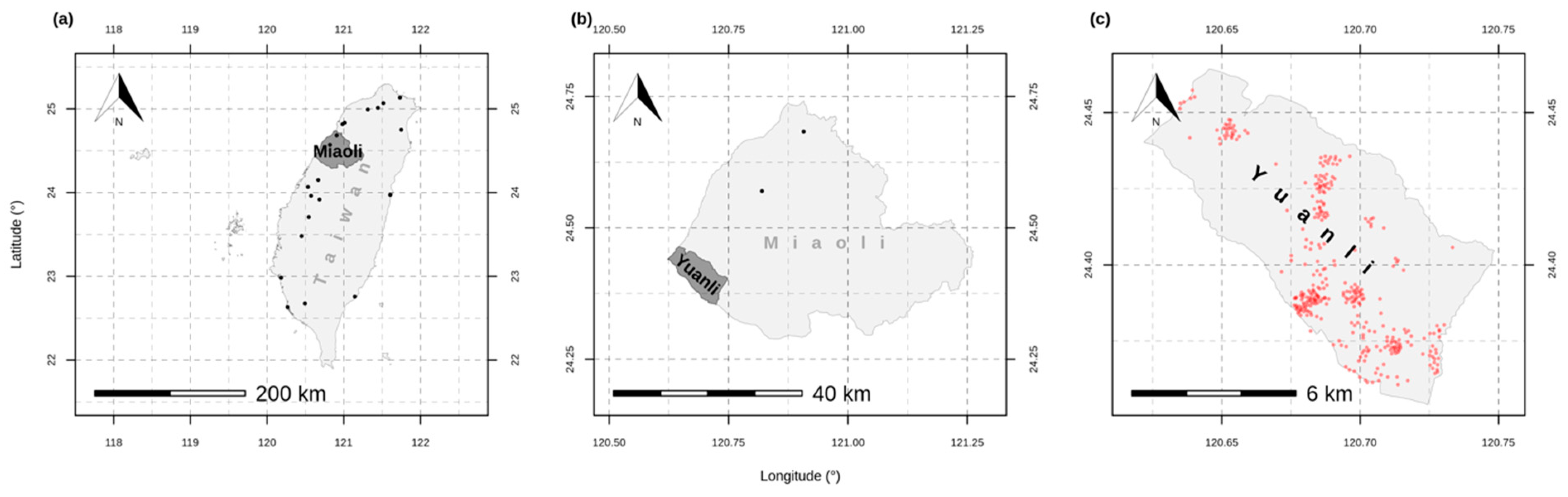
We examine the relationship between NICE valuations, at a rural socio-ecological production landscape scale in Miaoli, Taiwan, for two survey subgroups defined by k-means with correspondence analysis and principal component analysis. Survey data from a PPGIS mapping exercise, an analysis using the Social Values for Ecosystem Services [21] methodology, and Google Maps data were used to address three objectives: (1) Examine the relationship between highly valued NICE areas and cultural places, and in relation to each NICE value; (2) Determine which NICE values are associated with farms within the study area; and (3) Compare results of NICE valuations for the two survey subgroups of local farmers by their knowledge and experience levels as defined by social influence variables (i.e., age, formal education, farming experience, and organic training) that affect how ecological conservation and biodiversity value are perceived within their socio-ecological production landscape [55].

2.1. Study Area

Miaoli county is situated on the industrial west coast of the Taiwan island, which was accurately referred to as ‘Ilha Formosa’ by 16th century Portuguese mariners [57], and is one of East Asia’s economic “tigers” [58]. Spanning a total area of 1820 km2, Miaoli county relies on agricultural production unlike its two neighboring counties to the north and south, whose local economies are linked to its large science park and robust industrial zone. The county includes reserve areas for leopard cat conservation and sustainable land-use, as well as hiking tourist destinations [59]. In the southwestern corner of Miaoli county is Yuanli township, locally known as ‘Miaoli’s granary’, which has a total area of 68 km2 and a population of 46,939 (January 2017) [60] (Figure 1). In this study, Yuanli township is considered a rural SEPL defined as a “dynamic mosaic of managed socio-ecological systems producing a bundle of ecosystem services for human well-being” [12]. The SEPL concept refers to the traditional Japanese rural landscape called ‘satoyama’, and is currently embraced by the international community, and resonates with Taiwanese rural farmers while also appealing to urban intellectuals and policy makers for use as a common language of communication [61]. Yuanli township is considered a satoyama-like landscape [55] with relatively few environmental characteristics, and relatively homogeneous landscape classes—mostly a micro mosaic of agricultural land cover types. A rectangular-shaped mix of agricultural land and villages throughout the Snow Mountain foothills and its forest cut across Yuanli township along a northwest to southeast diagonal. The Da-An River borders Yuanli on its south and the coast along its western edge. As the Snow Mountain Range alluvial fan has been corroded by rivers, Miaoli County terrain is divided into plains, wolds, tablelands, and mountains [62]. Yuanli township is mostly plains at the base of the nearby mountains. The edaphic properties of the Yuanli study area can be characterized based on Mukhtar’s et al. [63] findings. Of the forest, fallow land, and crop land soils, mean temperature is 23.12 degrees Celsius. For forest soil, pH ranges from 5.03 to 5.63; total organic carbon ranges from 12.68 to 18.64 g/kg; and total nitrogen ranges from 1.24 to 1.25 g/kg. For fallow land soil, pH ranges from 6.35 to 6.42; total organic carbon ranges from 8.83 to 17.20 g/kg; and total nitrogen ranges from 0.97 to 1.40 g/kg. For crop land soil, pH ranges from 5.58 to 6.45; total organic carbon ranges from 12.27 to 14.32 g/kg; and total nitrogen ranges from 1.30 to 1.47 g/kg.

2.2. Spatial Data

Convenience sampling, a frequently used type of sampling in cross-cultural studies and social science studies, is largely influenced by availability and cost efficiency [64]. The sample of the population used reflects those who the researcher had access to at a moment in time while still trying to maintain representativeness in the sample population, thus striking a balance between rigor and practicality [65]. Convenience sampling is the preferred sampling method for many small-scale investigations of rural study areas in Taiwan, due to limited research funding and time constraints [66]. A convenience sample was comprised of farmers who were available and reachable by the study area’s local Agricultural Production and Marketing Group (APMG), a sub-organization of the Miaoli District Agricultural Research and Extension Station, Council of Agriculture, Executive Yuan. In Taiwan, APMGs are the way that the national-level agricultural governing body is able to exercise administrative functions at the local level, further sub-managed by crops (e.g., rice farmers in Miaoli county may belong to a local rice-specific versus a taro-specific APMG). These groups aim to increase agricultural product value and develop advanced processing techniques [66]. Respondent data used in this study was obtained using a structured questionnaire with a mapping exercise similar to the data collection methods used in Social Values for Ecosystem Services (SolVES 3.0) [67]. Specifically, participants were asked to allocate a total of 100 percent across seven NICE values that are found within their landscape: Aesthetic, Recreational, Educational, Historic-Cultural, Spiritual-Religious, Ecological Conservation, and Life Sustaining. Table S1 shows the NICE value types used in this study and in the SolVES application with value descriptions. Additionally, in a group setting, participants identified source locations of the values that they made allocations to, by marking on a printed map of the Yuanli study area; and identified marked locations by writing the location names, or writing down what their mapped markings referred to (hereby referred to as “named location”). That is, participants identified places within their landscape in the Yuanli study area that they valued in terms of the seven NICE values. For each of the seven NICE values, two locations were named. Demographic information was also collected (with 23 questions total) related to a farmer ’s socio-demographic profile, land ownership status, trust relationship with consumers, local observed levels of irrigation pollution, and farm operations and management. Specifically collected was information on respondents’ age, level of formal education attained, years of farming experience, and government-sponsored organic training received. These latter four variables were selected to determine sub-groups considering Petway et al. [55] and showed that for a demographically similar sample population in the same study area, these four variables were responsible for influencing farmers’ decisions to engage in conservation practices for agricultural biodiversity. The questionnaire was co-designed and administered in Mandarin Chinese by the study area’s local APMG representative and study researchers. The questionnaire and results were later translated into English. Prior to collecting farmers’ voluntary responses, farmers gave their informed consent, and research details were explained. Results were anonymized, and mapped points were digitized then cross-checked by either geocoding the written named locations with Google’s Geocoding API [68], or directly inputting the named location in Google Maps. Following data cleaning, 338 mapped data points and corresponding value allocations from 34 farmers were retained for further analysis. This small population of farmers is similar to previous studies [69].

2.3. Respondent Sub-Groups
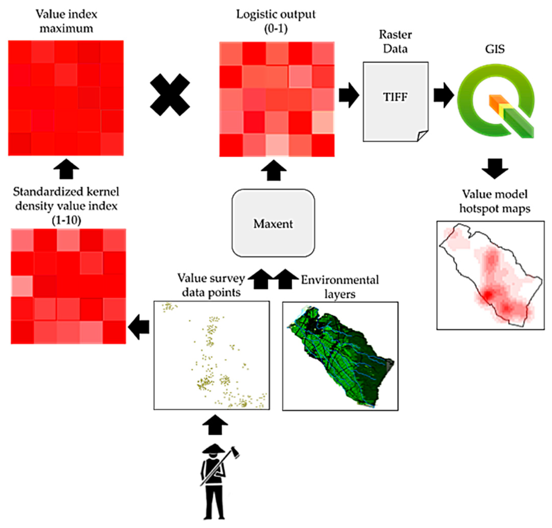
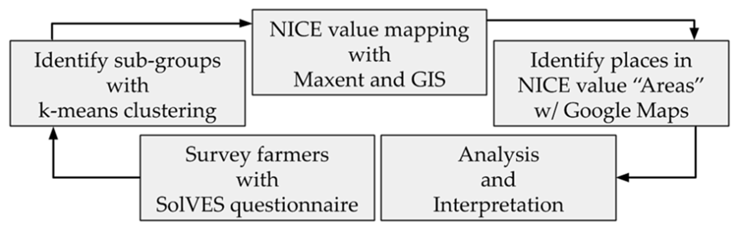
Subgroups are defined in this study using two methods to determine if delineated groups were identifiable in the respondent data based on four variables demographically associated with each respondent and considered social variables that influence an individual’s environmental concern and pro-environmental behavior in general [56]. Firstly, the ‘kmeans’ function in R [70] was used to cluster the respondents’ data into two groups so that the sum of squares from points to the assigned cluster centers are minimized [70] based on the Hartigan and Wong [71] algorithm. To assess the grouping in an ordination plot, the ‘rda’, ‘envfit’ and ‘ordiplot’ functions in the ‘vegan’ R package [72], were then used to perform a principal component analysis of the demographic data, fit the original demographic variables as vectors to aid interpretation, and finally display the groups and fitted vectors in an ordination plot. The rda function is based on Legendre and Legendre’s [73] algorithm in which a Chi-square transformed data matrix is subjected to ordinary, unweighted linear regression on constraining variables. The fitted values then undergo correspondence analysis (CA) performed via unweighted singular value decomposition (SVD). Secondly, R-package ‘FactoMineR’ [74] function ‘PCA’ was used to conduct a principal component analysis (PCA) on the dataset, and package ‘factoextra’ [75], was then used to produce a ggplot2-based visualization [75] of the computed the PCA results. By orthogonally transforming the dataset to explain the variance-covariance structure through linear combinations, PCA can reveal patterns evident in the dataset of how the respondents differ in terms of the four variables. While both methods, using k-means with CA or using PCA, are related and can both be based on the SVD algorithm, plotted results may yield conceptually different information. This is since CA uses relative values when respondent data are described by categorical (qualitative) variables, while PCA uses values when respondent data are described by quantitative variables [74]. For this reason, we applied two methods to validate subgroup delineations if both results concur.

2.4. Mapping

Social Values for Ecosystem Services, SolVES, [21] runs best on a Microsoft Windows operating system, and uses Esri ArcGIS 10.0 software; its Spatial Analyst Extension for working with grid-based data; and Maxent maximum entropy modeling software, version 3.3.3k. For this reason, this study used R [70] to execute a mapping method similar to the SolVES 3.0 ‘value mapping model’ tool [76] to obtain results. Survey data points were transformed into spatial point vectors. Kernel Density Estimation (KDE) of surfaces was performed for each of the seven NICE values based on the available spatial data points that respondents named for each value. Kernel density surfaces were not weighted by the respondents’ percent allocations since some did not provide complete allocations. In the SolvES value mapping model tool [76], using non-weighted kernel density surfaces is a valid option. After performing KDE, the maximum values across the seven values were identified for each cell and recorded in a single maximum grid which was standardized to range from one to ten. Maxent then generates logistic value layers (ranging from 0 to 1) using all identified locations across all seven NICE values. The Maxent logistic output is then multiplied with the maximum grid to estimate the overall social value. Maxent value map outputs were then used as inputs for compiling maps with QGIS Geographic Information System version 3.8.1-Zanzibar [77] (Figure 2).
Specifically, we used the R package ‘maxnet’ (version 0.1.2) [78] to calibrate a maximum entropy model based on mapped landscape value-features, random background points, and eight environmental variables. We calibrated 25 replicate models, each being trained on a subsample of 200 mapped value-features and 1600 random background points. The eight variables included the first three principal components (explaining 94.37% of the total variation) of ten climatic variables (cloud cover, temperature, and precipitation). Cloud cover [79] included mean, intra-annual SD and inter-annual SD and was downloaded from earthenv.org. Temperature and precipitation data [80] included mean annual temperature, isothermality (ratio of daily to annual variation in T), maximum and minimum temperature, annual precipitation, and wettest and driest month precipitation. The remaining five variables comprised the majority (categorical) and Shannon diversity of geomorphological landforms and vector ruggedness measure [81], land cover (categorical) downloaded from NASA [82], the MODIS Land Cover Type Product (MCD12Q1) [83] at 250 m resolution, and water distance which was computed in QGIS from the HYDROSHEDS river network data [84]. The resulting predictions were average using the mean.

3. Results

This study measured seven NICE values by deriving maps based on a combination of farmers’ spatial and nonspatial responses to preference questions about their SEPL; and based on variables determined to be socially influential to their decisions to sustain ES and conserve biodiversity with farming practices [55], in order to determine if groups defined by differing combinations of four social influence variables likewise make valuations of the nonmaterial-intangible benefits within their landscape in observably differing ways characterized by spatial patterns. Table S2 shows farmers’ responses to questionnaire items of interest including those that were used to distinguish between the two subgroups.

3.1. Nonmaterial-Intangible Cultural ES Value Allocations

As part of the mapping exercise, farmers were asked to allocate 100 percent among seven NICE values in the first portion of the structured questionnaire. While these valuations were not applied to the weighted measures when mapping, the responses show that of the seven NICE values, Educational, Historic-Cultural and Ecological Conservation, were the top three “highly valued” (i.e., receiving 100 and 80, 50, and 40 percent, respectively) at least once (Table S3). However, total sums of allocations indicate that Educational, Ecological Conservation and Life Sustaining were most valued over all (Table S4). The least valued were Aesthetic (4.14%), Spiritual-Religious (3.68%) and Recreation (3.22%). That is to say, these were the NICE values that received the most zero allocations (Table S3) and the lowest total sums (Table S4).

3.2. Respondent Subgroups

Similar subgroups emerged using both partitioning clustering with a k-means algorithm followed by CA method; and PCA method. The two groups that emerged, were delineated by their level of formal education attained, a variable that was also negatively correlated with government-sponsored organic training received, farming experience, and age. In this study, the ”YoungEd” group is defined as being the younger and more educated group, whereas the “OldEx” group is the older group with more farming experience. The grouping analysis results show evident patterns in the data in terms of how the individual farmers differed by social influence variables. Clusters returned by the k-means algorithm were used to color two groups of individuals (Figure S1). This delineation of groups is verified using principal component analysis (PCA) results (Table 2), visualized in Figure S2. The individuals are represented by their projections, whereas the variables are represented by their correlations [85]. These biplots also show how social influence variables correlate so that a positive correlation is implied in smaller angles as these variables are grouped together; negative correlations in larger angles or plotted in opposing sides of the origin; and no correlations at 90° angles. Figure S2 shows the degree of importance among the four social influence variables as well as the level of education variations within the YoungEd and OldEx groups.
The total contribution of a variable to PC1 and PC2, is calculated as contrib = [(C1 * Eig1) + (C2 * Eig2)]/(Eig1 + Eig2), where C1 and C2 are the contributions of the variable on PC1 and PC2, respectively; and Eig1 and Eig2 are the eigenvalues of PC1 and PC2, respectively. Cos2 is a reflection of the quality of representation of the variables on the factor map. For further information on this visualization, refer to R-package ‘factoextra’ [75] which extracts and visualizes results from R-package ‘factoMineR’ [74].

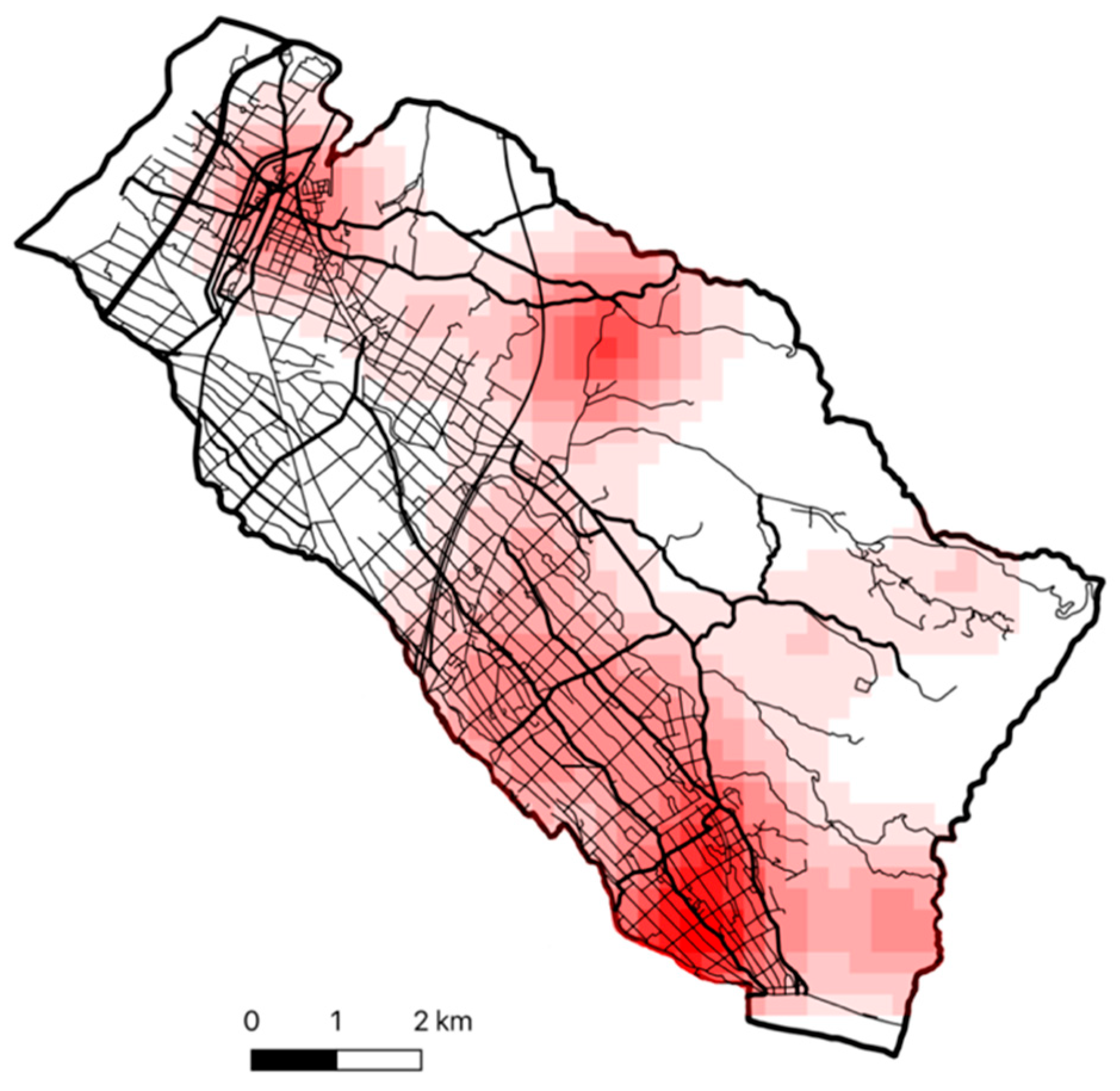
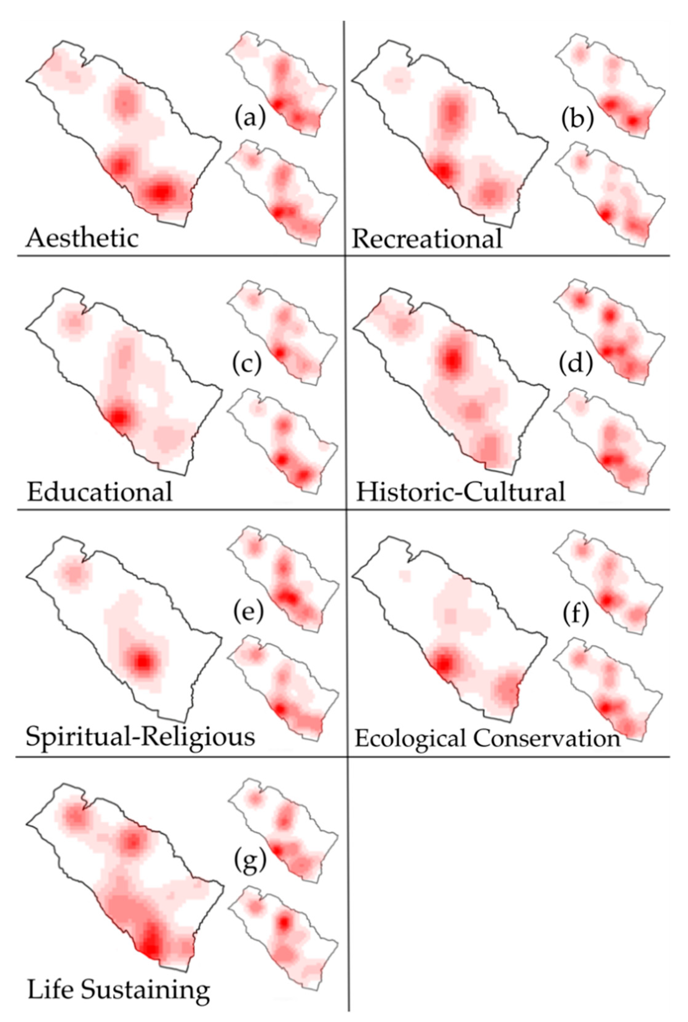
3.3. Mapping Nonmaterial-Intangible Cultural ES Value Totals

A total of seven NICE values were measured and mapped, as shown in Figure 3. Total hotspot maps generated in this study are the products of log. However, the Maxent surface with max grids across values are “weighted” in a way—they are equally weighted. Specifically, scaling to 1–10 was performed individually and not across the set of seven NICE values. Therefore, each individual value map ranged from 1 to 10 in integer. The maximum grid, hence, is an equally weighted representation of maxima across all value maps This is similar to scaling of variables in PCA to avoid undue dominance of individual layers. Based on mapped results, areas were defined with Google Maps as follows: “Area 1” is the coastal harbor area in Yuanli’s northwest corner; “Area 2” is slightly southeast of Area 1 and is downtown proper where the township government offices are located, as well as a community college, high school, and train station; “Area 3” is further southeast of Area 2 and a residential community at a slightly higher elevation where there is also an elementary school and a Farmers’ Association branch office; “Area 4” is south of Area 3 and in the southcentral agricultural hub where well-known organic farms are located; “Area 5” is southeast of Area 4 and in the southeastern corner with riverside, agricultural, and forest land at the mountain base moving into higher ground; “Area 6” is east of Area 5 and is higher elevation forest area on the backside of the mountain (Figure 4). For Yuanli farmers, these seven NICE values are located in Areas 3, 4, and 5; and to a lesser degree, Areas 2 and 6. In line with previous studies that have mapped NICE values, differences between the two subgroups were observed in point assignments that may relate to environmental characteristics within the ES-provisioning landscape [53]. More insight may be found, however, in the landscape’s cultural characteristics.
Specifically, Aesthetic value for the YoungEd group has a larger mapped area, with higher densities in southern agricultural places of the study area (Areas 4 and 5); whereas for the OldEx group, Areas 4 and 5 were not as dense, with high density limited to mostly Area 4, though Aesthetic value was mapped in the northern parts of the study area including coastal places (Areas 1 and 2) which was not a mapped location for the YoungEd group. See Figure 5a.
Recreation value has higher density patterns in southern agricultural places (Areas 4 and 5) for YoungEd than for OldEx overall, with higher densities in Area 5; density patterns are slightly more distributed for OldEx, who mapped more Recreation value in places between Areas 3 and 5, whereas the YoungEd mapped higher densities in places downtown (Area 2) than OldEx. This may indicate a difference in how both groups recreate, such that for YoungEd, recreational activities are not only enjoyed in natural settings but also in urban centers and include activities such as shopping and going to restaurants. See Figure 5b.
Educational value has the highest density pattern overall in the agricultural south (Area 4) for YoungEd. For OldEx, however, the highest densities were at Areas 3, 4, and 5. Though YoungEd mapped lesser density in Area 5 than OldEx, the group mapped a higher density of Educational value in Area 2 than OldEx. That is, both groups mapped Educational value in agricultural places but YoungEd mapped less Educational value in Area 5 where the natural reserve is located, and more in Area 2 downtown places when compared to OldEx. On the other hand, OldEx mapped less Educational value in the downtown area, where the community college and library are located. See Figure 5c.
Historical-Cultural value was mapped in the highest densities in Areas 2, 3, and 5 for YoungEd, with the highest in Area 3. For OldEx, the highest densities were mapped in southeast agricultural places (Area 4). For both groups, Historic-Cultural value mapped densities were similar to Aesthetic value maps. However, YoungEd tended to map more Historical-Cultural value than the OldEx group who have (arguably) lived through more history. See Figure 5d.
Spiritual-Religious value was denser in Areas 3 and 4 for YoungEd than elsewhere, and was mapped more densely overall when compared to OldEx. For OldEx, the highest densities were mapped in agricultural places in the southeast only (Area 4). Interestingly, for OldEx, their Spiritual-Religious value map’s density pattern is most similar to their Recreation value map; whereas for YoungEd, their Spiritual-Religious value map is most similar to their Ecological-Conservation value map, and even their Aesthetic value map. See Figure 5e.
Ecological Conservation value is mapped in a less distributed pattern for YoungEd than for OldEx; although for both groups, high densities were mapped at agricultural places in the southeast (Area 4) and even in the downtown area (Area 2). YoungEd mapped more Ecological Conservation value in Area 5 than OldEx. See Figure 5f.
Life Sustaining value maps were the most dissimilar between the two groups, with YoungEd mapping high densities in Area 4 (and to lesser degrees Areas 3 and 5); while OldEx mapped high densities in Area 3. OldEx, however, mapped Life Sustaining value in the coastal area (Area 1) while YoungEd did not. YoungEd, however, mapped more Life Sustaining value in Area 5 (which includes the natural reserve and riverside places) while OldEx did so to a lesser degree. See Figure 5g.

3.4. Area Differences When Mapping Nonmaterial-Intangible Cultural ES Values

Differences between the two groups’ spatially explicit valuations were also visualized (see Supplementary Material). Overall differences for seven total values mapped between the two groups were most pronounced in the way that values were mapped in Area 4 and 5. For Aesthetic value, the differences are greatest between YoungEd and OldEx groups in the way values were mapped in Area 5. YoungEd mapped more value in Area 5 places than OldEx (Figure S3a). Similarly, for Recreation value, differences were most prominent in Area 5 mapped values. YoungEd mapped more Recreation value in Area 5 than OldEx (Figure S3b). For Educational value, the most notable difference is seen in Area 3. YoungEd mapped Educational value in a more distributed pattern than OldEx. YoungEd also mapped some Educational value in Area 1 which OldEx did not (Figure S3c). For Historic-Cultural value, the greatest difference in mapping is seen in Area 3 followed by Area 2. YoungEd mapped more Historic-Culture value in these areas than did OldEx (Figure S3d). For Spiritual-Religious value, mapping differences are greatest in Area 4. Though both groups mapped Spiritual-Religious values in Area 4, the YoungEd value map was more distributed in Area 4 than the OldEx map (Figure S3e). For Ecological Conservation value, the mapping difference was greatest in Area 6. Though both groups mapped Ecological Conservation value in Area 5 near Area 6, YoungEd mapped more in Area 6 (Figure S3f). For Life Sustaining, the greatest mapping difference was in Area 4 due to YoungEd mapping more Life Sustaining value in this area than OldEx (Figure S3g).

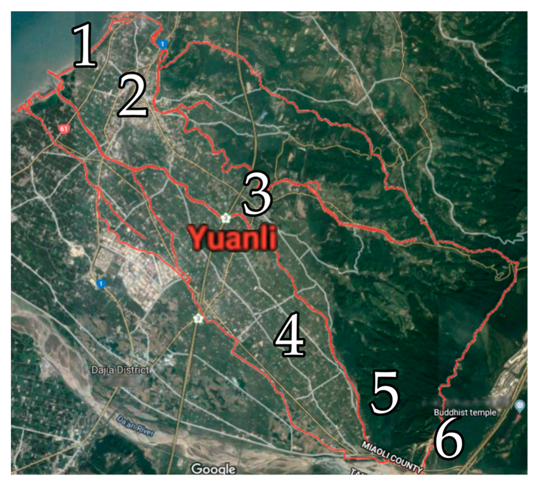
3.5. Identifying Places within the Cultural Landscape with Google Maps

Respondents mapped points and named locations, in most instances referring to specific places that are well-known and catalogued in Google Maps as ‘Place IDs’. Place IDs are available for “most locations, including businesses, landmarks, parks, and intersections” [86]. Some respondents’ named locations were unmappable such as ‘fresh air’, or ‘Da’An mountain’ in general. Respondents mapped points and named locations in Area 1, referring to two places on the coast: a coastal park and a bridge which is a local tourist attraction (Table S5). Respondents mapped points and named locations in Area 2, the downtown area, referring to seven places (Table S6). Three of the seven places were related to education (schools and a college association). The other four places include: a library, a Farmers’ Association branch office, a place of worship, and a restaurant. Respondents mapped points and named locations in Area 3, referring to 11 places (Table S7), one of which did not have a specific single-point location (i.e., the Yuanli River). Five places are related to rice farms (3 farms/fields, 1 rice museum, and 1 observation deck overlooking fields). Two places were schools, and one scenic place was located inside of a school. The remaining places included a memorial center, a public park, a Farmers’ Association branch office in an historic building, and a temple. Respondents mapped points and named locations in Area 4, referring to 11 places (Table S8). Five places are related to rice farms, three places of worship, a school, a kiln with gardens, and a community do-it-yourself workshop. Respondents mapped points and named locations in Areas 5 and 6, referring to one place each: the Huoyan Mountain Natural Reserve, and its trailhead (Table S9).

4. Discussion

4.1. Overview

Figure 6 is an overview of the study process. By indexing NICE values that were spatially intersected with land cover raster data, we show the relative concentration of values by subgroups on the physical landscape at a socio-ecological production landscape scale.
According to a visual assessment of the value maps of the total sample and both subgroups, Area 4 (followed by Area 5 then 3) are intensely valued locations within the landscape that are sources of multiple NICE values. That is, for Yuanli farmers, Area 4 is where there is the most capacity to provide public benefit and to represent meaningful places [53]. This is in line with Smith and Sullivan [87], who reported that ES are highly valued by farmers. For the YoungEd subgroup, all seven NICE values were located at high density in Area 4. For the OldEx subgroup, all NICE values except Life Sustaining were located at high density in Area 4. This exception, however, may be due to the way that the term ‘Life Sustaining’ sounds much like the name of a place in Area 3 (a memorial hall). Upon closer inspection of which places in Area 4 refer to farmers’ mapped and named locations, we found that most places in Area 4 were farms and places of worship. While Area 4 itself is relatively homogenous in terms of landscape characteristics, some features may have contributed to valuations. Two places, for example, are situated at the base of the nearby mountains. However, it is more likely that the area valuations were made for the places themselves rather than for the landscape featuring the places nearby.
This weak link between NICE valuations and environmental characteristics has also been reported by Van Berkel and Verburg [88], who question if NICE values are even usefully parameterized with spatial proxies. Results for this study also revealed that farming practices may influence farmers’ valuations of their landscape. While the landscape in this study is a micro mosaic of predominantly peri-urban agricultural land, and most of the farmers have lived their lives there, this observation is in line with past studies that have shown that residents in small communities demonstrate a keen sense of place and a highly developed ability to differentiate locations with NICE value [35]; and that local familiarity is key to making these valuations [69]. Our study demonstrates an initial step in unravelling how NICE valuations are made within a small-scale landscape class with limited heterogenity; how they are related to the cultural places within it; and how they are related to respondents’ farming practices. This is in stark contrast with recent studies, such as vanRiper et al. [53], which associated NICE value within a public national protected area, free of residential communities, where the land cover is diverse with multiple environmental characteristics.
Brown [89] argued that simply correlating values with environmental characteristics or landscape features insufficiently explains the associations derived from frequency distributions. That is to say, the causal relationship between NICE valuation and environmental characteristics remains inconclusive. Brown [89] also reported significant negative spatial association between NICE values and landscapes with agricultural croplands, and further, that all NICE values were underrepresented in agricultural and cropland classes. Yet, within SEPLs in Asia, rice cultivation dominates the majority of agricultural systems [90] and rice farming takes various forms. Unlike Sherrouse et al. [21], who used environmental characteristics (e.g., a river), Brown and Branbyn [91] concluded that specific landscape classes better explain the relationships between ES value and the landscape. However, the land use pattern in SEPLs is often observed to be a micro mosaic pattern of agricultural land cover types that includes paddy fields, terraced paddy fields, farmland, woodlands, grasslands, residential areas, ponds, and irrigation canals that are affected by water conditions and micro-topography; that historically require intense management by a decreasing and aging rural population [90]. By taking a place-based approach therefore, meanings and attachments within local contexts and conditions can be taken into account [9,59] within this micro mosaic of agricultural land at the SEPL scale since neither environmental characteristics nor landscape classes are explanatory enough. Our findings also contribute to research on NICE valuations of agricultural landscapes by showing that using a place-based approach [7,89] to understand the context-specific cultural aspects may explain NICE valuations more so than using preference survey data and environmental data alone at the SEPL scale.

4.2. Grouping

A previous study [55] defined farmers’ ‘life experiences’ as the combination of three socially influential variables [56]: farmer age, farming experience, and organic training received, to contrast with farmers’ level of formal education achieved. Similarly, our grouping results indicate that the subgroup YoungEd were younger and more educated than subgroup OldEx who had more life experience overall. OldEx were older with more experience from years of farming and government-sponsored organic training. While training could be considered education, we considered education to be school-taught, formal education. Government-sponsored organic farming training represents both current societal norms and the transmission of subjective norms [56,92], so that farmers with more organic training had also received a sense of the current social expectations of farming “behavior” for agricultural producers [55]. Assuming that more recent environmental concepts are transmitted via formal education, we hypothesized that younger, more educated farmers’ NICE valuations of their landscape would reflect their academically-acquired environmental concepts more so than the older, less educated, though more experienced, group. However, we found that mapping differences for the total of seven NICE values did not differ greatly by hotspot areas (Figure S4). That is, both groups’ total mapped NICE values were similarly distributed within the socio-ecological production landscape. In addition, specifically, for both groups, Area 4 was mapped as a place of high value for all values, with one exception to be discussed shortly. Yet, mapping differences became apparent when comparing group maps for each individual NICE value (Figures S5 and S6). Furthermore, these differences are observable in the way that both groups mapped individual NICE values to areas within the landscape.

4.3. Mapping

When looking at the underlying environmental characteristics that are assumed to underpin the measured NICE values, our findings show that the highly valued Area 4 is not incredibly diverse in itself in terms of environmental characteristics, though very diverse in terms of the different NICE value it provides. In fact, it is relatively homogenous as agricultural land. Areas 5 and 6 do, however, contribute to the SEPL’s overall biodiversity as being the area with forest and a source of Ecological Conservation value; while Area 1 is by the coast and Areas 2 and 3 contain built-up land which also adds to the overall landscape’s heterogeneity in terms of Historic-Cultural value. While both groups mapped Aesthetic value to similar Areas, YoungEd mapped the highest intensity of Aesthetic value to places in Areas 4 and 5; whereas OldEx mapped the highest intensity of Aesthetic value to places in Area 4. This may be a direct reflection of lifestyle. Especially, since YoungEd includes the HuoYan Mountain natural reserve in both its Aesthetic value as well as in its highly valued areas for Recreation. OldEx values the HuoYan Mountain Natural Reserve and its trails to a lesser degree for both Aesthetic and Recreational value. Whether the YoungEd’s Aesthetic and Recreation valuation of Area 5 (i.e., HuoYan Mountain Natural Reserve area) is due to experiential understanding or theoretical (i.e., time spent hiking and enjoying views vs. a conceptual understanding of the area based on its function) cannot be determined. Conversely, however, the OldEx group mapped more areas with a high intensity of Educational value including the HuoYan Mountain Natural Reserve, which YoungEd did not. The value of Area 5, then, seems to be a difference in the functional use of the HuoYan Mountain Natural Reserve for both groups of farmers. Lyytimaki et al. [93] reported that lifestyle can be seen in the behavioral patterns of consumption, recreation, work, and religious activities such that people experience and perceive nature in a great variety of ways as a result of their held attitudes and preferences that also stem from their lifestyle. The YoungEd group mapped more Areas of high intensity for both Historic-Cultural and Spiritual-Religious value than the OldEx group. In the case of Historic-Cultural value, farmers’ age may be directly influential. Most of the older farmers have also lived in the study area for their entire lives as farmers, and so years of living and working as farmers may influence their valuation of Area 4 (places that are mostly farms) such that Area 4 contains their personal history and culture. The YoungEd group, however, have been taught history rather than living through it, and can identify representations of historic and cultural traces in their landscape. An example of this is that YoungEd valued Areas with places that include buildings from the Japanese Occupation Era, or a local restaurant in the vicinity of Yuanli’s ‘Old Street’. That the OldEx group only mapped Spiritual-Religious value at a high intensity in Area 4 also attests to this notion that the OldEx group, who represent farmers who have spent their lives dedicated to farming, attribute deep personal meaning to farms alone.

4.4. Future Studies

Google ratings were not used in any statistical analysis in this study. Instead they are used in the descriptive analysis as a validation of the farmer responses. Comparing value maps to the respondents’ named locations in Google Maps, however, additionally provided insight into the accuracy of Google Maps’ algorithms that identify place types, in addition to insight into how the broader population of Google Map users who rate and review places, value places named by farmers. Google Maps is also heavily invested in mapping ‘places of interest’, which are more often than not commercial and tourist sites thereby embedding monetary valuations of landscapes by highlighting commercial and consumer interactions [94]. While ratings are user-generated, Google Maps “places” are often those of commercial interest and so the Google Maps digital landscape may accurately reflect only some—not all—nonmaterial and intangible aspects of cultural ES. Since Google Maps has already assumed a level of infrastructure [95] that may be perpetuating bias (which is often assumed that algorithms and artificial intelligent solutions to handling big data avoid), Google Maps data may also be used in future studies to identify any potential biases that are being transferred from our physical reality to algorithmic behavior. For example, traditional Indigenous naming conventions for highly valued cultural places (e.g., Danggu in Australia a.k.a. The Geikie Gorge) are not represented in Google Maps nor is there a formal mechanism for public involvement [94] though users can add places to Google Maps in a limited way. That is, since “automated systems discriminate by default” [96], we should ensure AI in such contexts as mapping our digital landscape, as a reflection of our real-world valued landscapes, are trained with various types of data including that from farming knowledge sources [97]. Future studies may investigate the quality of place ratings as an indicator of NICE value for specific place types for example. Or even, comparing Google Maps’ assigned place type to locals’ own designation of a place. For example, in this study, some respondents named location for Historic-Cultural value identified in Google Maps, returned a place type ‘restaurant’ with low ratings and reviews, most likely left by out-of-towners. However, this place’s local importance is not reflected in the business listing, since businesses often need to pay for more elaborate listings. Google Maps data may also be used for an investigation similar to that of Carvallo and Escalona [98], who looked at the way environmental characteristics were included in the names of Chilean municipality places as a proxy indicator for NICE valuations.

4.5. Limitations

This study is not without limitations. Some farmers’ named locations for NICE values were not mappable (e.g., Da’An River in general, or ‘the fresh air around us’). These named locations were not mapped but added to an understanding of the farmers’ view of their own landscape. Land cover data that does not include the various types of agricultural land within a SEPL misrepresents the landscape as seemingly homogenous. Though not available for this study, using high resolution land cover data representative of a micro mosaic of agricultural-related land cover types may provide more enriching discussions. Further, when a landscape has various land cover types, but the study population only moves around within one or two types, the landscape characteristics’ influence on the way valuations are made, is minimized. Rather, the places within these landscapes (which may be in relation to different configurations of environmental characteristics) may have cultural relevance regardless of the nearby environmental characteristics or the land use class. Furthermore, bandwidth parameters used when generating Maxent products affect the extent of the heat map appearance.

5. Conclusions

While participatory mapping is a popular way to identify socially valued ES hotspots to inform policy [89]; and while NICE studies have primarily focused on natural features [99], currently established methods for hotspot mapping using correlated preference survey data and environmental data may not accurately relate why these hotspots have value at the SEPL scale. Metrics such as ‘distance to river’ are often used in methods such as SolVES [21] that aim to draw a conclusive causal relationship between people’s valuations of NICE value and the landscape characteristics underpinning the experienced benefits, but may not be well suited for landscapes that are predominantly “lived in”, filled with “lived values” [29], and micro mosaics of heterogeneity where land cover variation and environmental characteristics are not as apparent at small scales as the cultural landscape and the many cultural places within it. Additionally, while past studies that map NICE value have sought to associate specific values with specific environmental characteristics or landscape classes, within a small scaled SEPL, in which the entire landscape is a source of NICE value to some degree—reveals that areas within the landscape provide places of differing cultural functions even when the landscape itself is relatively absent abundant natural features. Furthermore, that many of the named locations are man-made features is also consistent with studies reporting that built features are also sources of NICE value [99].
In this paper, we demonstrated that with the application of a place-based approach to expand the social data used in established methods for identifying nonmaterial-intangible cultural ecosystem service (NICE) value in rural agricultural socio-ecological production landscapes (SEPLs), we can better understand how farming practices, knowledge, and experience influence NICE valuation among farmers. This insight is valuable for promoting organic farming as a targeted management practice for conserving agricultural biodiversity and ES. For example, our findings suggest that environmental variables (or landscape classes) are not explanatory enough since local groups may not understand their own landscape solely in terms of environmental characteristics, but rather in terms of its functionality. That is, scientific and academic definitions may be dissimilar to local definitions of biodiversity in a rural SEPL, such that farmers’ understanding of the landscape’s biodiversity stems from the multi-functional places within the landscape itself rather than from species richness and diversity. Our findings also suggest that though the younger, more educated farmer group may have more academically acquired (and perhaps abstracted) environmental concepts and technology-related skills, the older experienced farmer group learned environmental concepts experientially and subsequently made more valuations that reflect practiced environmental concepts. Measures to increase technology-related skills (e.g., navigating on-line sales and record keeping) for the older experienced group, while also increasing hands-on environmental farming practices for the younger educated group may serve to level the valuation difference between the two groups. Additionally, this study demonstrates that the spatial quantification of NICE value within a rural, predominantly agricultural landscape can contribute to understanding the positive effects of farming practices on ES valuation in general, and further, that agricultural land is a source of multiple sub-categories of ‘cultural’ ES value.

Supplementary Materials

The following are available online at https://www.mdpi.com/2071-1050/12/2/699/s1. Table S1: Social value types used in this study and in the SolVES application (Sherrouse et al., 2011), Table S2: Profile of the total sample used in this study, Table S3: Frequency of percent allocations for seven nonmaterial-intangible cultural ecosystem service values, Table S4: Scores of percent allocations for nonmaterial-intangible cultural ecosystem service values, Figure S1: Biplot of individual groups defined by k-means clustering algorithm and social influence variable correlation plots, Figure S2: Biplot of principal component analysis results with variables and individuals, Figure S3: Nonmaterial-intangible value mapping differences between two groups, Table S5: Area 1 Google Maps places corresponding to respondent mapped and named locations, Table S6: Area 2 Google Maps places corresponding to respondent mapped and named locations, Table S7: Area 3 Google Maps places corresponding to respondent mapped and named locations, Table S8: Area 4 Google Maps places corresponding to respondent mapped and named locations, Table S9: Areas 5 and 6 Google Maps places corresponding to respondent mapped and named locations, Figure S4: Total of seven nonmaterial-intangible cultural ecosystem service valuations for Young Educated group and Old Experienced group, Figure S5: Young Educated group mapping results for seven nonmaterial-intangible cultural ecosystem service valuations, Figure S6: Old Experienced group mapping results for seven nonmaterial-intangible cultural ecosystem service valuations.

Author Contributions

The scope of this study was developed by Y.-P.L. The first manuscript draft was written by J.R.P. and Y.-P.L., and was substantially revised by J.R.P. and Y.-P.L. Modeling code was written by R.F.W. Visualizations were produced by J.R.P. and R.F.W. All authors have read and agreed to the published version of the manuscript.

Funding

The study was partially supported by the Council of Agriculture, Taiwan (No. 108AS-4.2.2-ST-a1).

Acknowledgments

The authors would like to thank the Council of Agriculture, Taiwan. The authors would like to extend our thanks to Zhen-Wei (Eartha) Hong for help with the survey data. Raw data available upon request.

Conflicts of Interest

The authors report no conflict of interest.

References

  1. Food and Agriculture Organization, Figure, Agricultural Land (% of Land Area) (1961–2016). Available online: https://data.worldbank.org/indicator/ag.lnd.agri.zs (accessed on 4 November 2019).
  2. Šūmane, S.; Kunda, I.; Knickel, K.; Strauss, A.; Tisenkopfs, T.; des Ios Rios, I.; Ashkenazy, A. Local and farmers’ knowledge matters! How integrating informal and formal knowledge enhances sustainable and resilient agriculture. J. Rural Stud. 2018, 59, 232–241. [Google Scholar] [CrossRef]
  3. Allen, K.E.; Quinn, C.E.; English, C.; Quinn, J.E. Relational values in agroecosystem governance. Curr. Opin. Environ. Sustain. 2018. [Google Scholar] [CrossRef]
  4. Raymond, C.M.; Kenter, J.O.; van Riper, C.J.; Rawluk, A.; Kendal, D. Editorial overview: Theoretical traditions in social values for sustainability. Sustain. Sci. 2019, 14, 1173–1185. Available online: https://link.springer.com/article/10.1007%2Fs11625-019-00723-7 (accessed on 30 October 2019). [CrossRef] [Green Version]
  5. Díaz, S.; Settele, J.; Brondízio, E. Summary for policymakers of the global assessment report on biodiversity and ecosystem services of the intergovernmental science-policy platform on biodiversity and ecosystem services. In Advance Unedited Version; Plenary of the intergovernmental science-policy platform on biodiversity and ecosystem services, seventh session; IPBES: Paris, France, 2019; Available online: https://www.ipbes.net/system/tdf/ipbes_7_10_add-1-_advance_0.pdf?file=1&type=node&id=35245 (accessed on 30 October 2019).
  6. Tadaki, M.; Sinner, J.; Chan, K.M.A. Making sense of environmental values: A typology of concepts. Ecol. Soc. 2017, 22, 7. [Google Scholar] [CrossRef]
  7. Small, N.; Munday, M.; Durance, I. The challenge of valuing ecosystem services that have no material benefits. Glob. Environ. Chang. 2017, 44, 57–67. [Google Scholar] [CrossRef]
  8. Millennium Ecosystem Assessment. Ecosystems and Human Well-Being; Island Press: Washington, WA, USA, 2005. [Google Scholar]
  9. IPBES. Global Assessment Report on Biodiversity and Ecosystem Services of the Intergovernmental Science—Policy Platform on Biodiversity and Ecosystem Services; Brondizio, E.S., Settele, J., Díaz, S., Ngo, H.T., Eds.; IPBES: Bonn, Germany, 2019. [Google Scholar]
  10. European Commission. Towards an EU Research and Innovation Policy Agenda for Nature-Based Solutions & Re-Naturing Cities. Final Report of the Horizon 2020 Expert Group on Nature-Based Solutions and Re-Naturing Cities; European Commission Directorate-General for Research and Innovation, Brussels. Available online: https://ec.europa.eu/programmes/horizon2020/en/news/towards-eu-research-and-innovation-policy-agenda-nature-based-solutions-re-naturing-cities (accessed on 30 October 2019).
  11. Ford, J.D.; Cameron, L.; Rubis, J. Including indigenous knowledge and experience in IPCC assessment reports. Nat. Clim. Chang. 2016, 6, 349–353. [Google Scholar] [CrossRef]
  12. IPSI Secretariat. The International Partnership for the Satoyama Initiative (IPSI): Information Booklet and 2016 Annual Report; United Nations University Institute for the Advanced Study of Sustainability: Tokyo, Japan, 2017. [Google Scholar]
  13. The Economics of Ecosystems and Biodiversity. Guidance Manual for TEEB Country Studies, Version 1.0. Available online: http://www.teebweb.org/media/2013/10/TEEB_GuidanceManual_2013_1.0.pdf (accessed on 2 November 2019).
  14. Costanza, R.; De Groot, R.; Braat, L.; Kubiszewski, I.; Fioramonti, L.; Sutton, P.; Grasso, M. Twenty years of ecosystem services: How far have we come and how far do we still need to go? Ecosyst. Serv. 2017, 28, 1–16. [Google Scholar] [CrossRef]
  15. Allen, K. Trade-offs in nature tourism: Contrasting parcel-level decisions with landscape conservation planning. Ecol. Soc. 2015, 20. [Google Scholar] [CrossRef] [Green Version]
  16. Fish, R.D. Environmental decision making and an ecosystems approach: Some challenges from the perspective of social science. Prog. Phys. Geogr. 2011, 35, 671–680. [Google Scholar] [CrossRef]
  17. Chan, K.M.; Goldstein, J.; Satterfield, T.; Hannahs, N.; Kikiloi, K.; Naidoo, R.; Woodside, U. Cultural services and non-use values. In Natural Capital: Theory & Practice of Mapping Ecosystem Services; Oxford University Press: Oxford, UK, 2011; pp. 206–228. [Google Scholar]
  18. Tenerelli, P.; Demšar, U.; Luque, S. Crowdsourcing indicators for cultural ecosystem services: A geographically weighted approach for mountain landscapes. Ecol. Indic. 2016, 64, 237–248. [Google Scholar] [CrossRef] [Green Version]
  19. Willemen, L.; Cottam, A.J.; Drakou, E.G.; Burgess, N.D. Using Social Media to Measure the Contribution of Red List Species to the Nature-Based Tourism Potential of African Protected Areas. PLoS ONE 2015, 10, e0129785. [Google Scholar] [CrossRef] [PubMed] [Green Version]
  20. Kirchhoff, T. Abandoning the Concept of Cultural Ecosystem Services, or Against Natural–Scientific Imperialism. BioScience 2019, 69, 220–227. [Google Scholar] [CrossRef]
  21. Sherrouse, B.C.; Clement, J.M.; Semmens, D.J. A GIS application for assessing, mapping, and quantifying the social values of ecosystem services. Appl. Geogr. 2011, 31, 748–760. [Google Scholar] [CrossRef]
  22. Chan, K.M.A.; Patricia, B.; Karina, B.; Mollie, C.; Sandra, D.; Erik, G.-B.; Rachelle, G. Opinion: Why protect nature? Rethinking values and the environment. Proc. Natl. Acad. Sci. USA 2016, 113, 1462–1465. [Google Scholar] [CrossRef] [Green Version]
  23. Calcagni, F.; Ana, T.; Amorim, M.; James JTimothy, C.; Johannes, L. Digital co-construction of relational values: Understanding the role of social media for sustainability. Sustain. Sci. 2019, 14, 1309–1321. [Google Scholar] [CrossRef]
  24. Rawluk, A.; Ford, R.; Williams, K. Value-based scenario planning: Exploring multifaceted values in natural disaster planning and management. Ecol. Soc. 2018, 23. [Google Scholar] [CrossRef]
  25. Jasper, O.; Kenter, L.; Norman, H.; Neil, R.; Ioan, F.; Katherine, N.I.; Mark, R.; Michael, C.; Emily, B.; Rosalind, B.; et al. What are shared and social values of ecosystems? Ecol. Econ. 2015, 111, 86–99. [Google Scholar] [CrossRef] [Green Version]
  26. Massenberg, J.R. Social values and sustainability: A retrospective view on the contribution of economics. Sustain. Sci. 2019, 14, 1233–1246. [Google Scholar] [CrossRef]
  27. van Riper, C.; Sophia, W.-S.; Lorraine, F.; Rose, K.; Michael, B.; Christopher, R.; Max, E.; Elizabeth, G.; Dana, J. Integrating multi-level values and pro-environmental behavior in a US protected area. Sustain. Sci. 2019, 1–14. [Google Scholar] [CrossRef] [Green Version]
  28. Raymond, I.J.; Raymond, C.M. Positive psychology perspectives on social values and their application to intentionally delivered sustainability interventions. Sustain. Sci. 2019, 14, 1–13. [Google Scholar] [CrossRef]
  29. Brear, M.R.; Mbonane, B.M. Social values, needs, and sustainable water–energy–food resource utilisation practices: A rural Swazi case study. Sustain. Sci. 2019, 14, 1363–1379. [Google Scholar] [CrossRef]
  30. Gould, R.K.; Pai, M.; Muraca, B.; Chan, K.M. He ʻike ʻana ia i ka pono (it is a recognizing of the right thing): How one indigenous worldview informs relational values and social values. Sustain. Sci. 2019, 14, 1213–1232. [Google Scholar] [CrossRef]
  31. Kim, U.; Yang, K.S.; Hwang, K.K. Indigenous and Cultural Psychology: Understanding People in Context; Springer Science & Business Media: Berlin/Heidelberg, Germany, 2006. [Google Scholar]
  32. Himes, A.; Muraca, B. Relational values: The key to pluralistic valuation of ecosystem services. Curr. Opin. Environ. Sustain. 2018, 35, 1–7. [Google Scholar] [CrossRef]
  33. Alessa, L.; Kliskey, A.; Brown, G. Social–ecological hotspots mapping: A spatial approach for identifying coupled social–ecological space. Landsc. Urban Plan. 2008, 85, 27–39. [Google Scholar] [CrossRef]
  34. Brown, G.; Raymond, C. The relationship between place attachment and landscape values: Toward mapping place attachment. Appl. Geogr. 2007, 27, 89–111. [Google Scholar] [CrossRef]
  35. Bryan, B.A.; Grandgirard, A.; Ward, J.R. Quantifying and exploring strategic regional priorities for managing natural capital and ecosystem services given multiple stakeholder perspectives. Ecosystems 2010, 13, 539–555. [Google Scholar] [CrossRef]
  36. Dramstad, W.E.; Tveit, M.S.; Fjellstad, W.J.; Fry, G.L. Relationships between visual landscape preferences and map-based indicators of landscape structure. Landsc. Urban Plan. 2006, 78, 465–474. [Google Scholar] [CrossRef]
  37. Raymond, C.M.; Bryan, B.A.; MacDonald, D.H.; Cast, A.; Strathearn, S.; Grandgirard, A.; Kalivas, T. Mapping community values for natural capital and ecosystem services. Ecol. Econ. 2009, 68, 1301–1315. [Google Scholar] [CrossRef]
  38. Milcu, A.; Hanspach, J.; Abson, D.; Fischer, J. Cultural ecosystem services: A literature review and prospects for future research. Ecol. Soc. 2013, 18. [Google Scholar] [CrossRef] [Green Version]
  39. Schulz, C.; Martin-Ortega, J. Quantifying relational values—why not? Curr. Opin. Environ. Sustain. 2018. [Google Scholar] [CrossRef]
  40. Kadykalo, A.N.; López-Rodriguez, M.D.; Ainscough, J.; Droste, N.; Ryu, H.; Ávila-Flores, G.; Sarkar, P. Disentangling ecosystem services and nature’s contributions to people. Ecosyst. People 2019, 15, 269–287. [Google Scholar] [CrossRef] [Green Version]
  41. UNU-IAS and IGES. IPSI Case Study Review—A Review of 80 Case Studies under the International Partnership for the Satoyama Initiative (IPSI); United Nations University Institute for the Advanced Study of Sustainability: Tokyo, Japan, 2015; Available online: https://collections.unu.edu/eserv/UNU:3371/IPSI_Case_Study_Review_2015.pdf (accessed on 20 November 2019).
  42. Hølleland, H.; Skrede, J.; Holmgaard, S.B. Cultural heritage and ecosystem services: A literature review. Conserv. Manag. Archaeol. Sites 2017, 19, 210–237. [Google Scholar] [CrossRef]
  43. Maes, J.; Paracchini, M.L.; Zulian, G.; Dunbar, M.B.; Alkemade, R. Synergies and trade-offs between ecosystem service supply, biodiversity, and habitat conservation status in Europe. Biol. Conserv. 2012, 155, 1–12. [Google Scholar] [CrossRef]
  44. Pagella, T.F.; Sinclair, F.L. Development and use of a typology of mapping tools to assess their fitness for supporting management of ecosystem service provision. Landsc. Ecol. 2014, 29, 383–399. [Google Scholar] [CrossRef] [Green Version]
  45. Gliozzo, G.; Pettorelli, N.; Haklay, M. Using crowdsourced imagery to detect cultural ecosystem services: A case study in South Wales, UK. Ecol. Soc. 2016, 21. [Google Scholar] [CrossRef] [Green Version]
  46. Liu, W.; Wang, J.; Li, C.; Chen, B.; Sun, Y. Using bibliometric analysis to understand the recent progress in agroecosystem services research. Ecol. Econ. 2019, 156, 293–305. [Google Scholar] [CrossRef]
  47. Cavanagh, R.D.; Broszeit, S.; Pilling, G.M.; Grant, S.M.; Murphy, E.J.; Austen, M.C. Valuing biodiversity and ecosystem services: A useful way to manage and conserve marine resources? Proc. R. Soc. B Biol. Sci. 2016, 283, 1635. [Google Scholar] [CrossRef] [Green Version]
  48. Pagiola, S.; Ruthenberg, I.M. Selling biodiversity in a coffee cup: Shade-grown coffee and conservation in Mesoamerica. In Selling Forest Environmental Services: Market-Based Mechanisms for Conservation and Development; International Institute for Environment and Development: London, UK, 2002; pp. 103–126. [Google Scholar]
  49. UNU-IAS and IGES. Sustainable Use of Biodiversity in Socio-ecological Production Landscapes and Seascapes and its Contribution to Effective Area-based Conservation; United Nations University Institute for the Advanced Study of Sustainability: Tokyo, Japan, 2018. [Google Scholar]
  50. Power, A.G. Ecosystem services and agriculture: Tradeoffs and synergies. Philos. Trans. R. Soc. B Biol. Sci. 2010, 365, 2959–2971. [Google Scholar] [CrossRef]
  51. Morgera, E.; Caro, C.; Duran, G. Organic Agriculture and the Law, Food and Agriculture Organization of the United Nations Legislative Study 107. Available online: http://www.fao.org/docrep/016/i2718e/i2718e.pdf (accessed on 22 May 2019).
  52. Plieninger, T.; van der Horst, D.; Schleyer, C.; Bieling, C. Sustaining ecosystem services in cultural landscapes. Ecol. Soc. 2014, 19. [Google Scholar] [CrossRef]
  53. Van Riper, C.J.; Kyle, G.T.; Sherrouse, B.C.; Bagstad, K.J.; Sutton, S.G. Toward an integrated understanding of perceived biodiversity values and environmental conditions in a national park. Ecol. Indic. 2017, 72, 278–287. [Google Scholar] [CrossRef]
  54. Issa, I.; Hamm, U. Adoption of organic farming as an opportunity for Syrian farmers of fresh fruit and vegetables: An application of the theory of planned behaviour and structural equation modelling. Sustainability 2017, 9, 2024. [Google Scholar] [CrossRef] [Green Version]
  55. Petway, J.R.; Lin, Y.P.; Wunderlich, R.F. Analyzing Opinions on Sustainable Agriculture: Toward Increasing Farmer Knowledge of Organic Practices in Taiwan-Yuanli Township. Sustainability 2019, 11, 3843. [Google Scholar] [CrossRef] [Green Version]
  56. Gifford, R.; Nilsson, A. Personal and social factors that influence pro-environmental concern and behaviour: A review. Int. J. Psychol. 2014, 49, 141–157. [Google Scholar] [CrossRef] [PubMed]
  57. Taiwan National Palace Museum Website. Available online: http://www.npm.gov.tw/exhbition/formosa/english/index.htm (accessed on 11 November 2019).
  58. CIA World Factbook. Available online: https://www.cia.gov/library/publications/the-world-factbook/geos/tw.html (accessed on 11 November 2019).
  59. Miaoli Government News. The Wizard of the Green: Leopard Cat Conservation. Available online: http://www.sanyi.gov.tw/eng/8-1-1.php?forewordID=258944&print=1 (accessed on 15 November 2018).
  60. Miaoli County Government Household Registration Service. Available online: https://mlhr.miaoli.gov.tw/ (accessed on 12 January 2020).
  61. Wei, S. The dilemmas of peach blossom valley: The resurgence of rice-terrace farming in Gongliao District, Taiwan. In The Living Politics of Self-Help Movements in East Asia; Palgrave Macmillan: Singapore, 2018; Available online: https://link.springer.com/chapter/10.1007/978-981-10-6337-4_9 (accessed on 3 September 2019).
  62. Miaoli County Government Website. Available online: https://www.miaoli.gov.tw/eng/cp.aspx?n=439 (accessed on 5 January 2020).
  63. Mukhtar, H.; Lin, Y.P.; Lin, C.M.; Petway, J.R. Assessing thermodynamic parameter sensitivity for simulating temperature responses of soil nitrification. Environ. Sci. Process. Impacts 2019, 21, 1596–1608. [Google Scholar] [CrossRef] [PubMed]
  64. Fons, J.R.; Van de Vijver, F.J. Cross-cultural Research Methods in Psychology. In International Encyclopedia of the Social & Behavioral Sciences, 2nd ed.; Wright, J.D., Ed.; Elsevier: Amsterdam, The Netherlands, 2015. [Google Scholar] [CrossRef]
  65. Baxter, K.; Courage, C.; Caine, K. Understanding Your Users: A Practical Guide to User Research Methods; Morgan Kaufmann Publishers: Burlington, MA, USA, 2015. [Google Scholar]
  66. Jiang, W.J.; Luh, Y.-H. Does higher food safety assurance bring higher returns? Evidence from Taiwan. Agric. Econ. 2018, 64, 477–488. [Google Scholar] [CrossRef] [Green Version]
  67. Sherrouse, B.C.; Semmens, D.J. Social values for ecosystem services, version 3.0 (SolVES 3.0)—Documentation and user manual: U.S. Geological Survey. Open File Rep. 2015, 1008, 65. [Google Scholar] [CrossRef]
  68. Google’s Geocoding API. Available online: https://developers.google.com/maps/documentation/geocoding/start (accessed on 8 August 2019).
  69. Soini, K.; Vaarala, H.; Pouta, E. Residents’ sense of place and landscape perceptions at the rural–urban interface. Landsc. Urban Plan. 2012, 104, 124–134. [Google Scholar] [CrossRef]
  70. R Core Team. R stats package v3.5.0. Available online: https://www.r-project.org/ (accessed on 18 January 2020).
  71. Hartigan, J.A.; Wong, M.A. Algorithm AS 136: A K-means clustering algorithm. Appl. Stat. 1979, 28, 100–108. [Google Scholar] [CrossRef]
  72. Oksanen, J. R Package Vegan Package v2.5-6. Available online: https://cran.r-project.org/package=vegan (accessed on 11 November 2019).
  73. Legendre, P.; Legendre, L. Numerical Ecology, 3rd ed.; Elsevier: Amsterdam, The Netherlands, 2012. [Google Scholar]
  74. Lê, S.; Josse, J.; Husson, F. FactoMineR: An R package for multivariate analysis. J. Stat. Softw. 2008, 25, 1–18. Available online: http://factominer.free.fr/more/article_FactoMineR.pdf (accessed on 12 November 2019).
  75. Kassambara, A.; Mundt, F.; R-Package, F. Extract and Visualize the Results of Multivariate Data Analyses. Available online: https://CRAN.R-project.org/package=factoextra (accessed on 12 November 2019).
  76. Semmens, D.J.; Sherrouse, B.C.; Ancona, Z.H. Using social-context matching to improve spatial function-transfer performance for cultural ecosystem service models. Ecosyst. Serv. 2019, 38, 100945. [Google Scholar] [CrossRef]
  77. QGIS Development Team. QGIS Geographic Information System Version 3.8.1-Zanzibar. Open Source Geospatial Foundation Project. Available online: http://qgis.osgeo.org (accessed on 11 December 2018).
  78. Steven, P. Maxnet: Fitting Maxent Species Distribution Models with glmnet. R Package Version0.1.2. Available online: https://CRAN.R-project.org/package=maxnet (accessed on 15 September 2019).
  79. Wilson, A.M.; Jetz, W. Remotely Sensed High-Resolution Global Cloud Dynamics for Predicting Ecosystem and Biodiversity Distributions. PLoS Biol. 2016, 14, e1002415. [Google Scholar] [CrossRef] [PubMed]
  80. Karger, D.N.; Conrad, O.; Böhner, J.; Kawohl, T.; Kreft, H.; Soria-Auza, R.W.; Zimmermann, N.E.; Linder, H.P.; Kessler, M. Climatologies at high resolution for the earth’s land surface areas. Sci. Data 2017, 4, 170122. [Google Scholar] [CrossRef] [PubMed] [Green Version]
  81. Amatulli, G.; Domisch, S.; Tuanmu, M.-N.; Parmentier, B.; Ranipeta, A.; Malczyk, J.; Jetz, W. A suite of global, cross-scale topographic variables for environmental and biodiversity modeling. Sci. Data 2018, 5, 180040. [Google Scholar] [CrossRef] [PubMed] [Green Version]
  82. Friedl, M.; Sulla-Menashe, D. MCD12Q1 MODIS/Terra+Aqua Land Cover Type Yearly L3 Global 500m SIN Grid V006 [Data set]. NASA EOSDIS Land Processes DAAC. 2015. Available online: https://lpdaac.usgs.gov/products/mcd12q1v006/ (accessed on 12 January 2020). [CrossRef]
  83. Sulla-Menashe, D.; Friedl, M.A. User Guide to Collection 6 MODIS Land Cover (MCD12Q1 and MCD12C1) Product; USGS: Reston, VA, USA, 2018. Available online: http://icdc.cen.uni-hamburg.de/fileadmin/user_upload/icdc_Dokumente/MODIS/mcd12_user_guide_v6.pdf (accessed on 8 November 2019).
  84. Lehner, B.; Verdin, K.; Jarvis, A. New global hydrography derived from spaceborne elevation data. AGU 2008, 89, 93–94. [Google Scholar] [CrossRef]
  85. Abdi, H.; Williams, L.J. Principal component analysis. Wiley interdisciplinary reviews: Computational statistics. Sci. Educ. 2010, 2, 433–459. [Google Scholar] [CrossRef]
  86. Google. Google Maps Place IDs. Available online: https://developers.google.com/places/place-id (accessed on 14 November 2019).
  87. Smith, H.F.; Sullivan, C.A. Ecosystem services within agricultural landscapes—Farmers’ perceptions. Ecol. Econ. 2014, 98, 72–80. [Google Scholar] [CrossRef]
  88. Van Berkel, D.B.; Verburg, P.H. Spatial quantification and valuation of cultural ecosystem services in an agricultural landscape. Ecol. Indic. 2014, 37, 163–174. [Google Scholar] [CrossRef]
  89. Brown, G. The relationship between social values for ecosystem services and global land cover: An empirical analysis. Ecosyst. Serv. 2013, 5, 58–68. [Google Scholar] [CrossRef]
  90. UNU-IAS. Socio-Ecological Production Landscapes in Asia; United Nations University Institute for the Advanced Study of Sustainability: Tokyo, Japan, 2018; Available online: https://satoyama-initiative.org/wp-content/uploads/2018/01/SEPL_in_Asia_report_2nd_Printing.web_.pdf (accessed on 22 November 2019).
  91. Brown, G.; Brabyn, L. An analysis of the relationships between multiple values and physical landscapes at a regional scale using public participation GIS and landscape character classification. Landsc. Urban Plan. 2012, 107, 317–331. [Google Scholar] [CrossRef]
  92. Vesely, S.; Klöckner, C.A. Global social norms and environmental behavior. Environ. Behav. 2018, 50, 247–272. [Google Scholar] [CrossRef]
  93. Lyytimäki, J.; Petersen, L.K.; Normander, B.; Bezák, P. Nature as a nuisance? Ecosystem services and disservices to urban lifestyle. Environ. Sci. 2008, 5, 161–172. [Google Scholar] [CrossRef] [Green Version]
  94. McQuire, S. One map to rule them all? Google Maps as digital technical object. Commun. Public 2019, 4, 150–165. [Google Scholar] [CrossRef]
  95. Plantin, J.C. Digital Traces in Context Google Maps as Cartographic Infrastructure: From Participatory Mapmaking to Database Maintenance. Int. J. Commun. 2018, 12, 18. Available online: https://ijoc.org/index.php/ijoc/article/view/5988 (accessed on 8 November 2019).
  96. Broussard, M. Artificial Unintelligence: How Computers Misunderstand the World; MIT Press: Cambridge, MA, USA, 2018. [Google Scholar]
  97. Lin, Y.P.; Petway, J.R.; Settele, J. Train artificial intelligence to be fair to farming. Nature 2017, 552, 334. [Google Scholar] [CrossRef] [PubMed] [Green Version]
  98. Carvallo, G.O.; Escalona, M.J. Toponyms as Proxy of Cultural Ecosystem Services: An example using chilean Municipality Names. Available online: https://www.researchgate.net/publication/329298786_TOPONYMS_AS_PROXY_OF_CULTURAL_ECOSYSTEM_SERVICES_AN_EXAMPLE_USING_CHILEAN_MUNICIPALITY_NAMES (accessed on 14 January 2020).
  99. Van Berkel, D.B.; Tabrizian, P.; Dorning, M.A.; Smart, L.; Newcomb, D.; Mehaffey, M.; Meentemeyer, R.K. Quantifying the visual-sensory landscape qualities that contribute to cultural ecosystem services using social media and LiDAR. Ecosyst. Serv. 2018, 31, 326–335. [Google Scholar] [CrossRef] [PubMed]
Figure 1. Study area of Yuanli Township, Miaoli County, Taiwan. (a) Taiwan map; (b) Miaoli county map; (c) Yuanli township map.
Sustainability 12 00699 g001
Figure 2. Nonmaterial-intangible value mapping process with Maxent used in this study. Adapted from Sherrouse and Semmens [67].
Sustainability 12 00699 g002
Figure 3. Total of seven nonmaterial-intangible cultural ecosystem service value hotspots for farmers in Yuanlin, Taiwan. Note: darkest red indicates highest intensity.
Sustainability 12 00699 g003
Figure 4. Screenshot of Google Maps render of Yuanli Township borders and rivers in red with area labels. Areas are defined as: Area 1 is coastal; Area 2 is downtown; Area 3 is residential at higher elevation; Area 4 is agricultural hub; Area 5 is riverside and natural reserve; Area 6 is backside of mountain. Map data attribution in accordance with Google Terms of Service: Google 2019, Maxar Technologies, CNES Airbus, TerraMetrica, Data SIO, NOAA, U.S. Navy, NGA, GEBCO, Landsat Copernicus imagery.
Sustainability 12 00699 g004
Figure 5. Mapped results for seven nonmaterial-intangible cultural ecosystem service (NICE) valuations. Note: For each NICE value map, left is Total surveyed population, top-right is Young Educated group, and bottom-right is Old Experienced group for (a) through (g).
Sustainability 12 00699 g005
Figure 6. Study flowchart. Note: Social Values for Ecosystem Services (SolVES; Sherrouse et al. [18]); Nonmaterial-Intangible Cultural Ecosystem Services (NICE) values refers to the seven values measured in this study; Geographic Information System (GIS).
Sustainability 12 00699 g006
Table 1. Nonmaterial-Intangible Ecosystem Service Value Sub-Categories of Globally Recognized Frameworks/Systems.
MATEEBCICESIPBES
(1) cultural diversity(1) aesthetic information(1) physical and experiential interactions(1) Regulating NCP
(2) spiritual and religious values(2) opportunities for recreation & tourism(2) intellectual and representative interactions(2) Nonmaterial NCP
(3) knowledge systems(3) inspiration for culture, art and design(3) spiritual and/or emblematic interactions(3) Material NCP
(4) educational values(4) spiritual experience(4) other cultural outputs
(5) inspiration(5) information for cognitive development
(6) aesthetic values
(7) social relations
(8) sense of place
(9) cultural heritage
(10) recreation and ecotourism
Note: Millennium Ecosystem Assessment (MA); the economics of ecosystems and biodiversity (TEEB); the Common International Classification of Ecosystem Services (CICES v4.3); Inter-governmental Platform on Biodiversity and Ecosystem Services (IPBES); ‘NCP’ is Nature’s Contribution to People.
Table 2. Principal Component Analysis Results of Variable Contributions to Components 1 and 2.
Dim.1ContribCos2Dim.2ContribCos2
edu−0.86529.2260.747−0.0710.5880.005
age0.91232.5120.831−0.1422.3100.020
farmexp0.80225.1760.644−0.48026.5680.231
orgtrain0.57813.0860.3350.78370.5340.613
Note: Dim.1 is principal component 1 (PC1); Dim.2 is principal component 2 (PC2); ‘edu’ is level of formal education attained; ‘farmexp’ is years of farming experience; ‘orgtrain’ is government-sponsored organic training received; ‘contrib’ is contribution of a variable; ‘cos2′ is the squared coordinates.

