On the Operational Flood Forecasting Practices Using Low-Quality Data Input of a Distributed Hydrological Model

Abstract

Low-quality input data (such as sparse rainfall gauges, low spatial resolution soil type and land use maps) have limited the application of physically-based distributed hydrological models in operational practices in many data-sparse regions. It is necessary to quantify the uncertainty in the deterministic forecast results of distributed models. In this paper, the TOPographic Kinematic Approximation and Integration (TOPKAPI) distributed model was used for deterministic forecasts with low-quality input data, and then the Hydrologic Uncertainty Processor (HUP) was used to provide the probabilistic forecast results for operational practices. Results showed that the deterministic forecasts by TOPKAPI performed poorly in some flood seasons, such as the years 1997, 2001 and 2008, despite which the overall accuracy of the whole study period 1996–2008 could be acceptable and generally reproduced the hydrological behaviors of the catchment (Lushi basin, China). The HUP model can not only provide probabilistic forecasts (e.g., 90% predictive uncertainty bounds), but also provides deterministic forecasts in terms of 50% percentiles. The 50% percentiles obviously improved the forecast accuracy of selected flood events at the leading time of one hour. Besides, the HUP performance decayed with the leading time increasing (6, 12 h). This work revealed that deterministic model outputs had large uncertainties in flood forecasts, and the HUP model may provide an alternative for operational flood forecasting practices in those areas with low-quality data.

1. Introduction

Floods are the most frequent type of natural disaster and pose a huge threat to society [1,2,3]. Historically, people have been trying to understand floods, fight against them, and manage them [2,3,4,5]. In the process of continuously searching for flood disaster prevention measures, people realized that hydrological forecasting can play an effective role in flood prevention and disaster reduction [6,7]. Hydrological forecasting is an important non-engineering measure in flood prevention and mitigation measures. It plays an important role in flood prevention and rescue, reducing flood losses and protection of water resources. It is based on the current understanding of the basic laws of the hydrological cycle by human beings and predicts future hydrological behaviors using applied science and technology. With the improvement of the level of computer application, the mathematical hydrological forecasting technique has made breakthroughs in theoretical research and has been applied to operational practice in many basins of world [8,9,10,11,12,13]. Overall, in current operational flood forecasts, forecasting accuracy has improved and the leading time has been extended. The information of forecasting results has been also enriched. These advances have largely supported flood prevention decisions [14,15,16].

Hydrological models are an important tool for hydrological forecasting. The development of hydrological models has undergone major stages, such as empirical models, black-box models, conceptual hydrological models and distributed hydrological models. From the beginning, only models with system concepts have gradually developed into models with physical foundations [14,17]. Theoretically, the distributed hydrological model could provide more reliable results than before when the model parameters were physically determined according thematic maps, field measurement, literature and catchment characteristics or hydrological behavior analysis [6,14]. Data in many regions of the world do not perfectly meet the requirement of distributed hydrological models, although these models have been simplified to some extent. The lack of model input is particularly serious in some developing countries [18,19,20]. For example, high resolution thematic maps of digital elevation model (DEM), soil type, land cover and geology are difficult to obtain in many regions of China, and generally, only coarse resolution (low spatial resolution) thematic maps downloaded from the Internet could be used for the application of distributed hydrological models [21,22]. Besides, although distributed hydrological models are applied, only the river discharge type observation data are available for model test [23]. This case does not reflect the value and advantages of applying distributed hydrological models. Therefore, in many cases in China, the accuracy of distributed hydrological models will not be significantly improved compared to lumped models [24,25].

The hydrological process is extremely complicated, and humans have a limited level of cognition of hydrological laws. The development of hydrological models inevitably involves uncertainties in model inputs, structures and parameters. The existence of these uncertainties will inevitably lead to uncertain results of flood forecasts [18,19,20,26,27]. Deterministic forecasting is often applied in current operational flood forecasting. It is impossible to quantify the uncertainty of the forecast results, and therefore it is not possible to make an objective assessment of the possible risks of flood control decisions. Therefore, the realization of probabilistic flood forecasting to quantitatively describe the uncertainty of the forecasting process has gradually become a trend in operational forecasts [13,18,19].

In this study, we used a physically based rainfall-runoff model, the TOPographic Kinematic Approximation and Integration (TOPKAPI) model, with coarse (low spatial resolution) thematic maps and discharge data as inputs for deterministic flood forecasting in a mountainous basin of the middle Yellow River. Furthermore, the TOPKAPI model was coupled with a general uncertainty analysis framework, the Hydrologic Uncertainty Processor (HUP), to conduct probabilistic flood forecasting considering uncertainties in deterministic forecasting results. This study could provide a reference for deterministic and probabilistic operational flood forecasting practices in similar basins. More importantly, this study will contribute to the operational flood forecasting practices research with low-quality data in some data-sparse regions, although the models used (i.e., TOPKAPI and HUP) have been frequently applied.

2. Materials and Methods

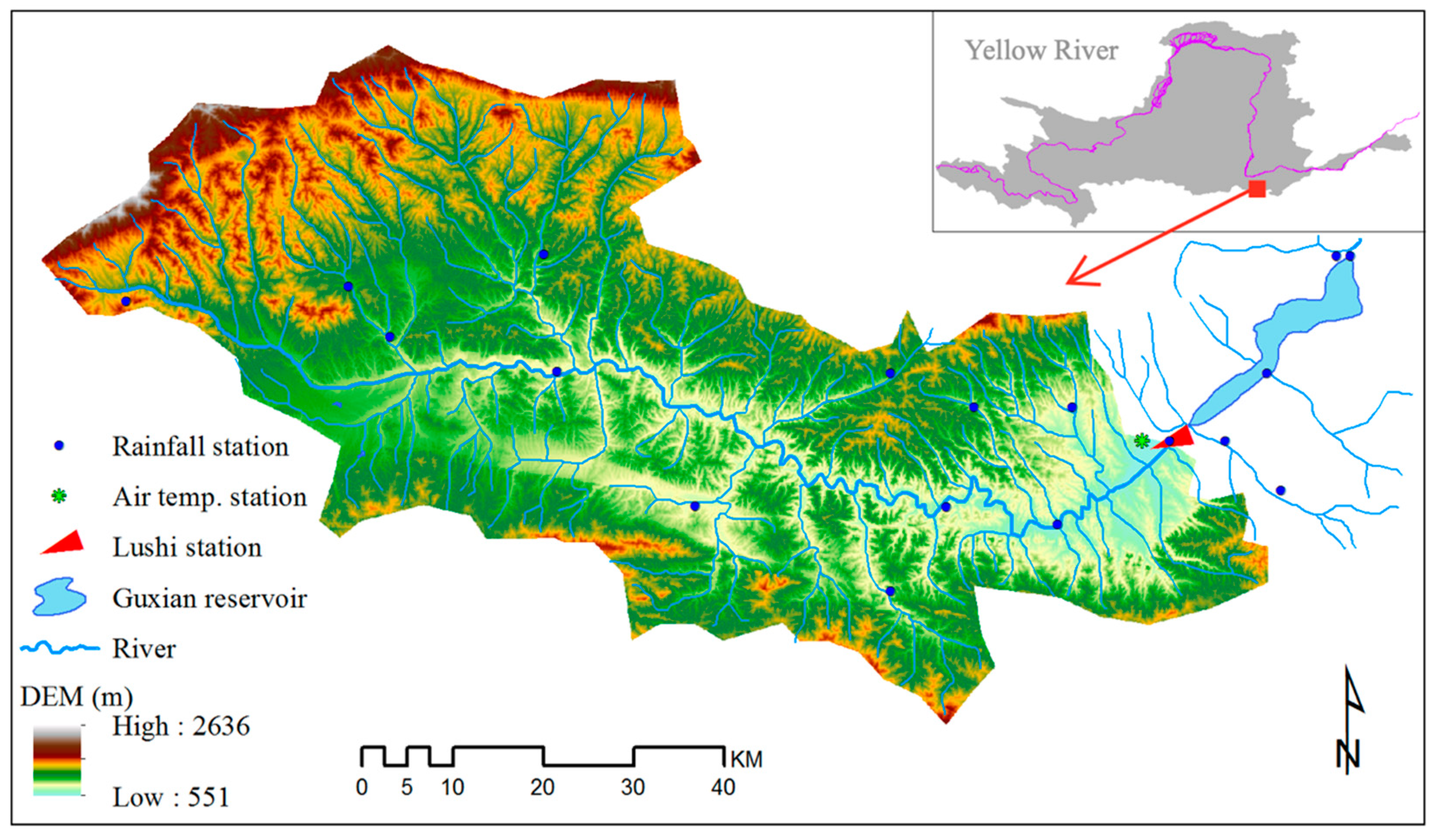
2.1. Study Basin

The drainage area above the Lushi hydrological station (Lushi basin) has a spatial extension of 4482 km² and could be viewed as the source area of the Yiluohe River (Figure 1). The Yiluohe River is a first tributary in the middle reaches of the Yellow River. The topography of the Lushi basin is complex, with landforms dominated by mountains and hills. Precipitation in the basin is characterized by uneven spatial and temporal distribution. On the spatial scale, mountainous areas are rainy zones, while river valleys and hills are less rainy zones. On the time scale, rainfall events are mainly concentrated in the flood season (June–October), accounting for more than 60% of the rainfall in the whole year, and occur in the form of heavy rain, which is characterized by high flood peaks, large floods and sharp rises and falls.

There are 13 rainfall stations and one air temperature station distributed within the basin. In this study, several rainfall stations outside the basin were also used in precipitation interpolation for providing reliable spatial estimates of precipitation. The Lushi hydrological station located at the basin outlet controls the streamflow process from the whole drainage basin.

2.2. Data

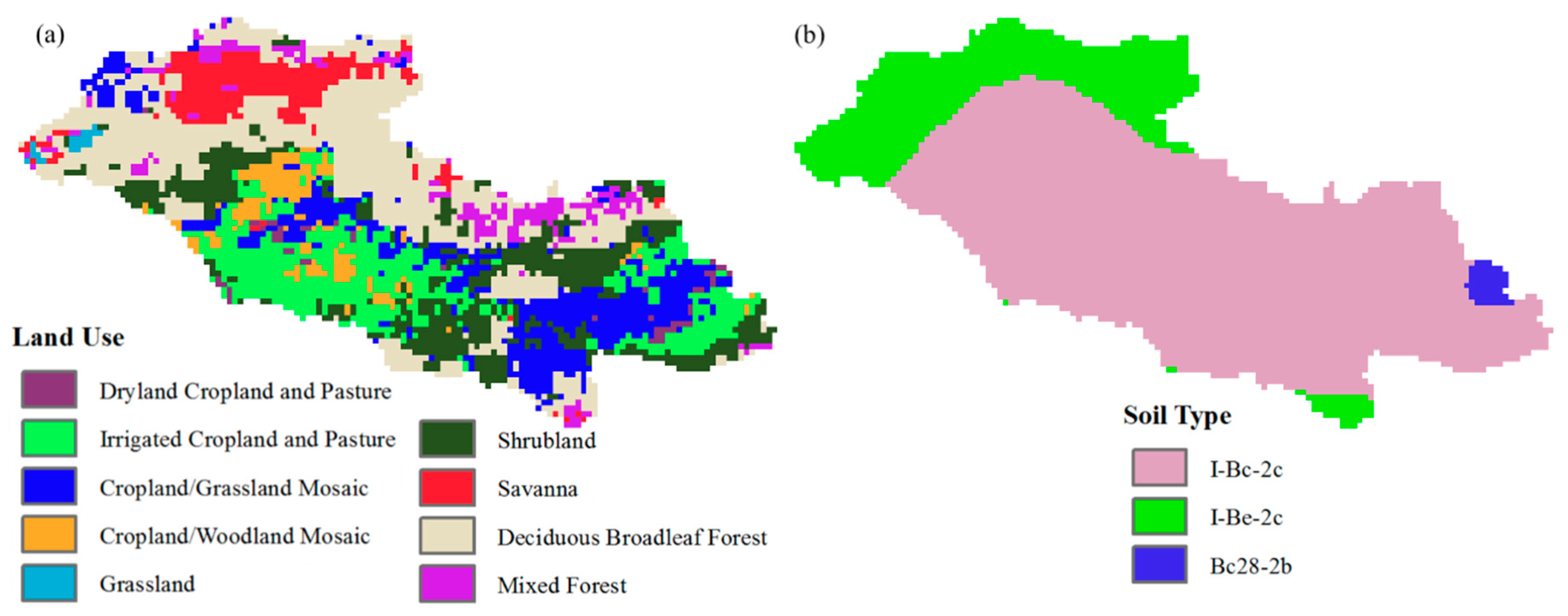
2.2.1. Thematic Maps

A DEM with a spatial resolution of 78 × 78 m and a land use map of the study area were provided by the Yellow River Conservancy Commission of the Ministry of Water Resources, P. R. China (YRCC-MWR). The source area of the Yiluohe River is located in a mountainous area with steep slopes, and its elevations range, approximately, from 551 m to 2636 m. The catchment is characterized by a central valley where the main river flow is receiving water from side tributaries flowing on the mountainside.

According to the land use map, the study basin is characterized by nine different types of land use (Figure 2a). The dominating land use of the Lushi basin is deciduous broadleaf forest with a percentage of 32%, followed by shrubland, irrigated cropland and pasture and cropland/grassland mosaic, which account for 18%, 17% and 15%, respectively. The remaining five types of land use have a smaller distribution area in the catchment, and the area percentages are all less than 10%.

The soil type map at a 1:5,000,000 scale was obtained from the Food and Agriculture Organization (FAO) of the United Nations. Only three soil types in the basin could be obtained from the data set (Figure 2b). The number of soil types is small, and the main type is soil I-Bc–2c with a percentage of 78%. Soil I-Be–2c mainly characterizes the mountains upstream at high elevations.

For the purpose of operational flood forecasting practice, the hydrological model was conducted at a spatial resolution of 1 × 1 km in the study basin. Thus, the thematic maps of DEM, land use and soil type were resampled to a 1 × 1 km resolution accordingly.

2.2.2. Hydrometeorological Data

The hydrometeorological database contains rainfall, discharge at Lushi hydrological station and air temperate data for the period of 1996 to 2008. The time steps of the original rainfall data are unequally spaced, and the steps in the flood season are mainly one hour to several hours, while the time steps in the non-flood season are mostly 1 day. The flood forecasts were conducted using hourly time steps in this study. Thus, observed rainfall measurements at different time steps were sampled using equal values to 1 h time steps. Point rainfall data have good quality control and were interpolated to each grid cell using the Inverse Squared Distance (ISD) technique. In fact, many popular rainfall interpolation methods do not particularly consider the influence of elevation factors, so the interpolation effect in mountainous areas is not as good as in plain areas. Previous studies [28,29,30,31,32] have proven that some spatial interpolation techniques (such as ISD, Kriging and others) may be superior under certain conditions (e.g., affected by data conditions and climatic conditions). The ISD method was chosen because we have compared and confirmed that the interpolation accuracy was better than the Block Kriging (BK) method in the period when data of some rainfall stations were missing, and the interpolation accuracy was comparable to the BK method in the rainfall data-rich period.

Air temperature at Lushi station was collected and interpolated with a lapse rate of −0.6 °C/100 m estimated using the 0.5 Degree Gridded Monthly China Surface Precipitation and Air Temperature Dataset (Version 2) [33]. This data product is developed by the Climate Data Center, China Meteorological Administration based on the data collected at 2472 climate stations and the Thin Plate Spline interpolation technique. The data quality is strictly controlled and can be used directly. The historical air temperature data were recorded at 6-h time steps (02:00, 08:00, 14:00, 20:00) and they include daily minimum and maximum values. The original temperature data were interpolated to hourly time steps for operational flood forecasting purposes.

Hourly discharge data were only available during the flood season. During the non-flood season, some discharge data are missing. In the non-flood season, when daily discharge was reported at Lushi hydrological station, the daily discharge was assumed constant over 24 h.

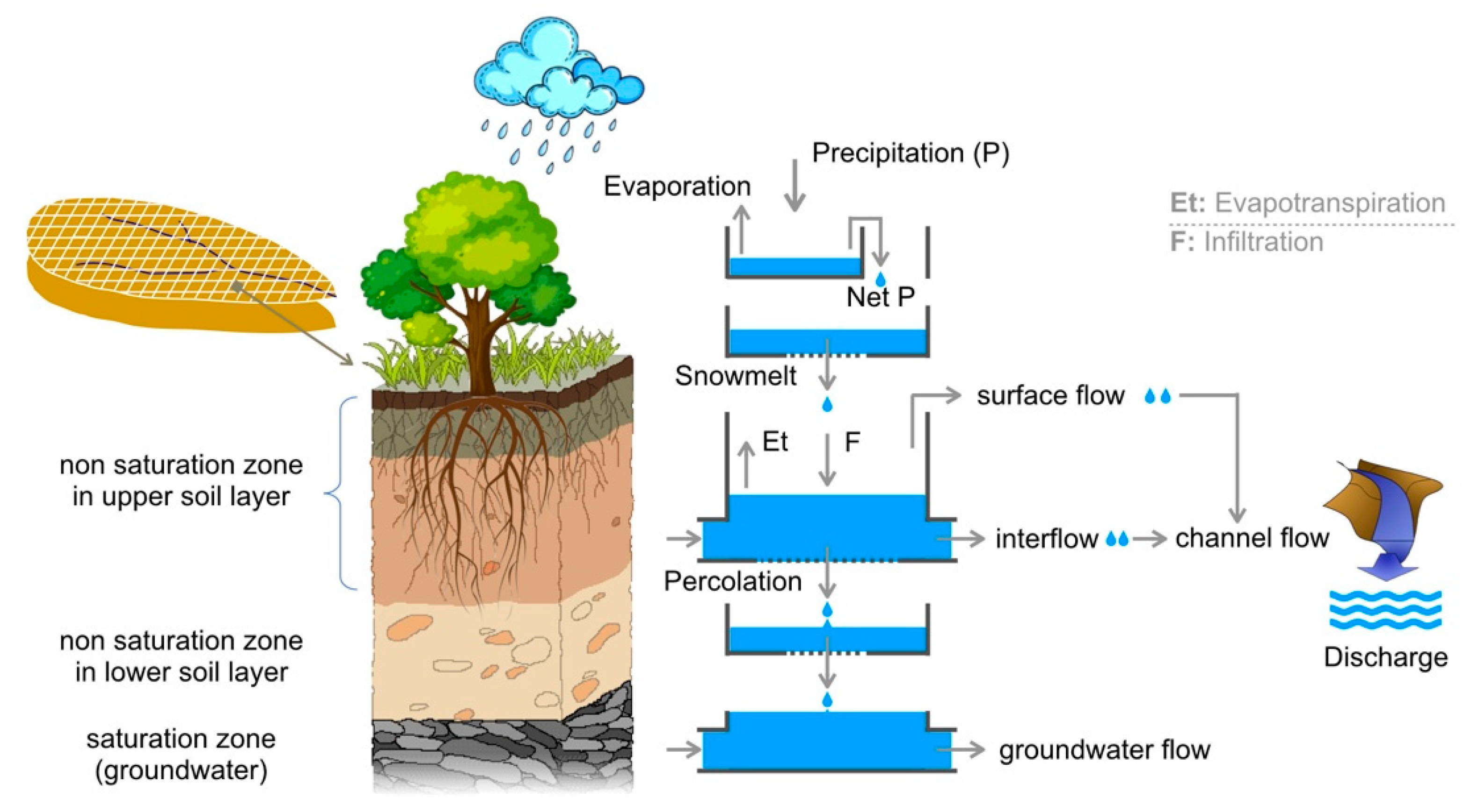
2.3. The Distributed Hydrological Model

A physically based rainfall-runoff model, TOPKAPI (TOPographic Kinematic Approximation and Integration) [21,34,35], was used for deterministic flood forecasts in the study basin. TOPKAPI uses three ‘structurally-similar’, zero-dimensional, non-linear reservoir equations to represent the drainage in the soil, the overland flow and the channel flow. The TOPKAPI structure is model lumping, preserving the process’ non-linearities and retaining the physically meaningful parameters. This enhances the model’s practicality in basins with low-quality data that cannot meet the requirement of fully distributed hydrological models, e.g., the Systeme Hydrologique Europeen (SHE) model [36,37]. The TOPKAPI parameters are reported as scale-independent and could be determined from digital elevation maps, vegetation or land use maps and soil type maps in terms of slopes, soil permeability, topography and surface roughness. The runoff production and routing processes are described on grid scales. The study basin is divided into several square grids and the calculation of runoff generation is conducted at each grid cell. Thus, the spatial variabilities of meteorological inputs (e.g., precipitation and air temperature) and model parameters could be considered. TOPKAPI is developed based on the saturation-excess runoff mechanism and includes five basic components, namely evapotranspiration, snowmelt, surface flow, interflow and channel flow (Figure 3). The model assumes that soil water percolation towards the deeper subsoil layers does not contribute to the basin discharge. It is acceptable for flood forecast cases because the response time of deep aquifer flow is so large for one specific storm event in a catchment. The percolation rate from the upper soil layer is assumed to increase as a function of the soil water content according to an experimentally determined power law [21].

In the calculation of interflow, the constant saturated hydraulic conductivity (K_s), along with depth in the non-saturation soil zone, is used. This implies the assumption that the total soil content integrated along the vertical profile with constant K_s does not differ strongly from the horizontal flux evaluated from the integration of the vertical soil moisture content profile. The total soil water content is addressed using the continuity equation and the dynamic equation and described in a non-linear reservoir equation. Surface flow only occurs in a grid cell when the soil is already saturated. In addition, water in the soil can exfiltrate on the surface as return flow due to a sudden change in hill slope or soil properties. Surface flow routing is described similarly to the soil component, according to the Kinematic approach, in which the momentum equation is approximated by means of the Manning’s formula. The interflow flow and the surface flow together feed the channel along the drainage network. The channel flow routing is described using the Kinematic non-linear reservoir, and two types of river reach, namely rectangular and triangular cross sections, could be considered.

The TOPKAPI model uses a simplified method to calculate evapotranspiration starting from air temperature and from other topographic, geographic and climatic information. Potential evapotranspiration can be computed for a given grid cell using the Thornthwaite equation [38] with the input data of air temperature and is further corrected as a function of the actual soil moisture content to obtain the actual evapotranspiration. A radiation estimate based upon air temperature is developed to represent the snowmelt module. In practice, the inputs to the module are precipitation, air temperature and the same radiation approximation which was used in the evapotranspiration module.

2.4. Hydrologic Uncertainty Processor

The Hydrologic University Processor (HUP) is a main sub-model within the Bayesian Forecasting System (BFS) proposed by R. Krzysztofowicz [39]. BFS is one of the most representative probabilistic forecasting models. It provides a general theoretical framework for probabilistic forecasting of hydrological variables. It combines the effects of various random factors on the forecasting results of hydrological models. It can be coupled with any hydrological model or forecasting scheme to obtain probabilistic forecasting results. Currently, BFS has been used in different river basins in the world [40,41,42,43,44,45]. BFS includes three sub-models: precipitation uncertainty processor (PUP), HUP and integrator (INT). Within the BFS framework, total uncertainty of hydrological forecasting is decomposed into two kinds of uncertainty: input and hydrological uncertainties. They are processed by PUP and HUP, respectively. BFS does not directly deal with the uncertainty of the model structure and model parameters. Instead, it takes the model output into consideration and can be coupled with any form of deterministic hydrological model. In view of the data limitation of the precipitation uncertainty analysis in our case, we do not consider the precipitation uncertainty, but only consider the hydrological uncertainty, and use the HUP model to realize the probability flood forecasting.

In the HUP model, H₀ is defined as the measured flow that is known at the time of forecasting. The variables H_n and S_n are the measured flow process and the flow process predicted by the deterministic hydrological model, respectively, and N is the leading time. The measured value of H_n and the estimated value of S_n are represented by h_n and s_n, respectively. For any time n and the observed value H_n = h_n, the prior probability function g_n and the likelihood function f_n could be synthesized using the total probability rule. According to Bayes’ theorem, the posterior density function of H_n under the condition of S_n = s_n is as [46]:

$${\varnothing }_n\left(h_n|s_n,h_0\right)=\frac{f_n\left(s_n|h_n,h_0\right)g_n\left(h_n|h_0\right)}{{\int }_{-\infty }^{\infty }{f}_n\left(s_n|h_n,h_0\right)g_n\left(h_n|h_0\right)d{h}_n}$$

(1)

In this study, the marginal distribution functions of the given measured discharge and the calculated discharge with the leading times (1, 6 and 12 h) were described by the log-Weibull distribution [39]. The parameters of the distribution could be estimated by the method of Moments. Using Equation (1), the probabilistic forecasting results could be obtained in the study basin.

2.5. Model Coupling

2.5.1. Model Combination of TOPKAPI and HUP

The TOPKAPI model is a deterministic hydrological simulation tool and was used for flood forecasting in this study to provide deterministic results of river discharge. HUP is a “model-free” uncertainty analysis framework that could be coupled with any deterministic models. The coupling between HUP and TOPKAPI is loose, not a form of coupling on the internal structure. Therefore, HUP only needs the output of the TOPKAPI model (such as the forecast flow process) as its input. Finally, the river discharge output of HUP is probabilistic (and could be further analyzed to provide a deterministic form).

In this study, therefore, TOPKAPI independently provides deterministic results, while HUP provides both deterministic and probabilistic results on the basis of the TOPKAPI outputs.

2.5.2. Performance Metrics

In the model simulations, $O_i$ and $S_i$ are defined as the observed and simulated discharges at the i-th time step, respectively, and n is the sample size. The variables $\overline{O}$ and $\overline{S}$ represent the mean values for the n-sized observed and simulated data series, respectively. For deterministic forecasts, the following four indices were used to evaluate the model’s performance in consecutive hydrological simulation or multi-flood-event simulation:

• Correlation Coefficient (CC)

  $$\mathrm{CC}=\frac{{{\displaystyle \sum }}_{i=1}^n\left(O_i-\overline{O}\right)\left(S_i-\overline{S}\right)}{\sqrt{{{\displaystyle \sum }}_{i=1}^n{\left(O_i-\overline{O}\right)}^2}·\sqrt{{{\displaystyle \sum }}_{i=1}^n{\left(S_i-\overline{S}\right)}^2}},$$

  (2)
• Mean Absolute Error (MAE)

  $$\mathrm{MAE}=\frac{1}{n}{{\displaystyle \sum }}_{i=1}^n\left|S_i-O_i\right|,$$

  (3)
• Nash–Sutcliffe Coefficient Efficiency (NSCE)

  $$\mathrm{NSCE}=1-\frac{{{\displaystyle \sum }}_{i=1}^n{\left(O_i-S_i\right)}^2}{{{\displaystyle \sum }}_{i=1}^n{\left(O_i-\overline{O}\right)}^2},$$

  (4)
• Index of Agreement (IOA)

  $$\mathrm{IOA}=1-\frac{{{\displaystyle \sum }}_{i=1}^n{\left(O_i-S_i\right)}^2}{{{\displaystyle \sum }}_{i=1}^n{\left(\left|S_i-\overline{O}\right|+\left|O_i-\overline{O}\right|\right)}^2},$$

  (5)

For the model performance evaluation of a specific flood event, the relative bias of flood peak (RBP) and the relative bias of flood volume (RBV) were also used:

$$\{\begin{array}{c}RBP=\frac{S_p-O_p}{O_p}\times 100\%\\ RBV=\frac{S_v-O_v}{O_v}\times 100\%\end{array},$$

(6)

where $S_p$ and $O_p$ are the values of peak discharge for simulated and observed samples, respectively, while $S_v$ and $O_v$ represent the volumes of a specific flood event for simulated and observed samples, respectively.

In the evaluation of probabilistic flood forecasts, the statistics of contained percent (CP) and dispersion index (DI) could be used [13,18,19]. The CP index measures the percentage of observations that are contained within the predictive uncertainty (PU) bounds at a given Confidence Interval (CI). The DI measures the average width of the predicted interval at a given CI after eliminating the influence of magnitude.

$$\{\begin{array}{c}CP=\frac{n_c}{n}\times 100\%\hfill \\ DI=\frac{1}{n}{{\displaystyle \sum }}_{i=1}^n\frac{Q_i^u-Q_i^d}{O_i}\hfill \end{array}$$

(7)

where n_c is the number of observed discharge samples enveloped by the PU bounds; $Q_i^u$ and $Q_i^d$ represent the PU bounds at the i-th time step. Theoretically, an ideal result of probabilistic forecasting should have the value of CP at a given CI close to the value of CI, and the value of DI should be as small as possible to ensure that the PU bounds are not too wide [13]. In this study, the PU bounds from 5% to 95% were calculated for flood events.

3. Results and Discussion

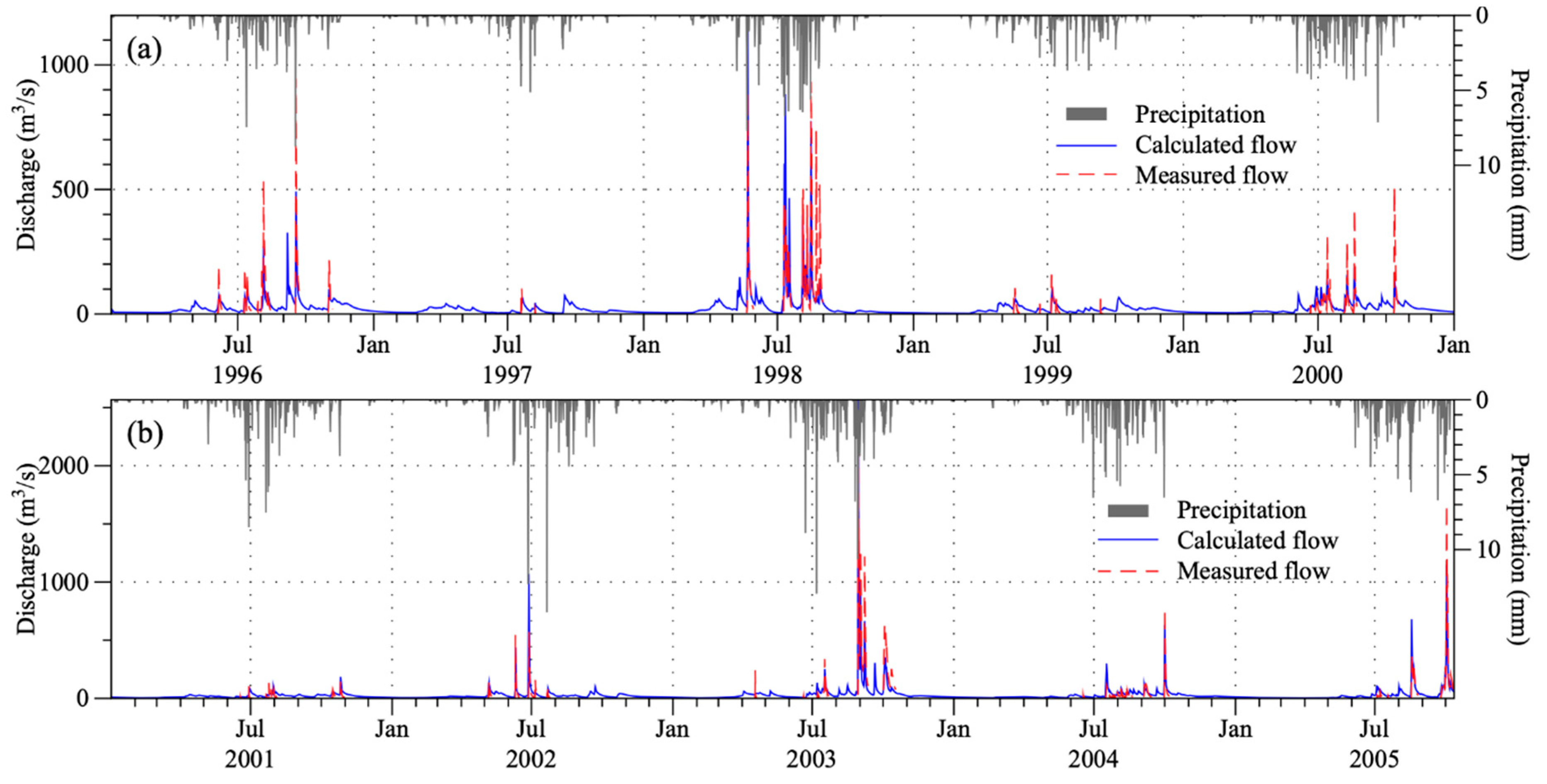
3.1. Model Calibration and Validation

The TOPKAPI model was calibrated in the Lushi basin using the hydrometeorological data for the period of 1996 to 2005; successively, the data for the period of 2006 to 2008 were used as a validation test. For flood forecasting purposes, hourly time steps were used. Since the TOPKAPI model is a physically distributed model at the theoretical level, the model parameters can be obtained through thematic maps, literature and catchment characteristics or hydrological behavior analysis. However, due to the coarse resolution of thematic maps and the complexity of underlying surface characteristics, the values of model parameters directly obtained from thematic maps, literature and catchment characteristics analysis would introduce obvious errors in the model results. To reproduce the behavior of the catchment, the initial values of the parameters from thematic maps, literature and catchment characteristics analysis were modified. Model simulated discharges were compared with observations at the Lushi station.

3.1.1. Parameters of the TOPKAPI Model

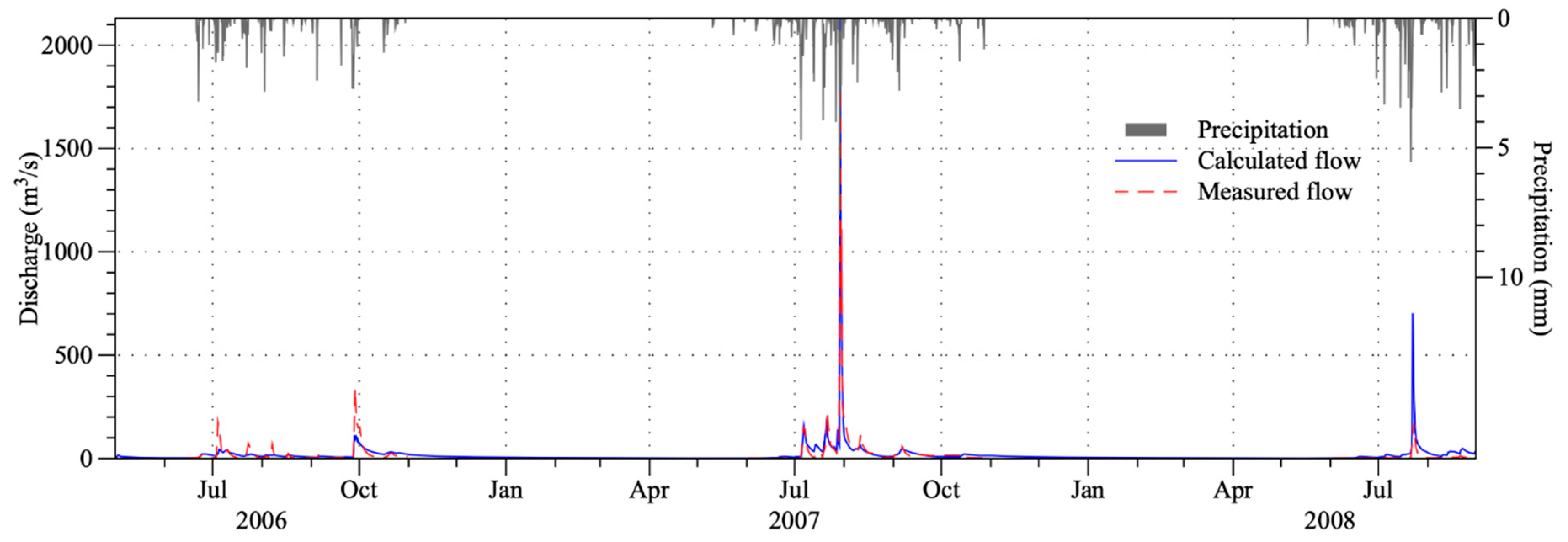
1. Evapotranspiration

TOPKAPI calculates potential evapotranspiration and actual evapotranspiration at each grid cell for each time step based on the soil water content. The minimum soil water content for having evapotranspiration was fixed at 20% of the soil saturation water content, while soil saturation that was above 80% of the actual evapotranspiration was equal to the potential evapotranspiration.

2. Soil Type Parameters

Hydrological behavior of the soil at each grid cell was characterized by hydro-geological parameters. The parameters for each soil type were obtained based on FAO soil classification, and the initial values of these hydro-geological parameters were retrieved from a previous TOPKAPI application study [35]. These initial values were used for model calibration in this study.

Table 1. Calibrated values of soil type parameters for the Lushi basin.

FAO Soil Type	Horizontal Permeability at Saturation (m/s)	Saturated Water Content	Residual Water Content	Soil Depth (m)	Horizontal Non-Linear Reservoir Exponent	Vertical Permeability at Saturation (m/s)	Vertical Non-Linear Reservoir Exponent
I-Bc–2c	2.19 × 10−3	0.423	0.303	0.85	2.5	2.19 × 10−7	23.8
I-Be–2c	9.27 × 10−4	0.39	0.27	0.55	2.5	3.27 × 10−7	18.5
Bc28–2b	7.67 × 10−4	0.33	0.21	1.35	2.5	7.67 × 10−8	17.2

shows the final calibrated values of the soil type parameters.

3. Land Use Parameters

The values of surface roughness and crop factors were obtained from literature according to the land use classification [35]. These parameter values were considered as the initial values and would be modified during the calibration procedure.

Table 2. Calibrated values of land use parameters for the Lushi basin.

Land Use Type	Manning Coefficient (s/m^(1/3))
Dryland cropland and pasture	0.08
Irrigated cropland and pasture	0.10
Cropland/grassland mosaic	0.12
Cropland/woodland mosaic	0.14
Grassland	0.12
Shrubland	0.13
Savanna	0.13
Deciduous broadleaf forest	0.19
Mixed forest	0.19

and

Table 3. Calibrated values of land use parameters for the Lushi basin.

Land Use Type	Crop Factors
	Jan	Feb	Mar	Apr	May	Jun	Jul	Aug	Sep	Oct	Nov	Dec
Dryland cropland and pasture	0.7	0.7	0.8	0.8	0.9	1.1	1.15	1	1	0.9	0.8	0.8
Irrigated cropland and pasture	0.7	0.7	0.8	0.8	0.9	1.1	1.15	1	1	0.9	0.8	0.8
Cropland/ grassland mosaic	0.7	0.7	0.8	0.8	0.9	1.1	1.15	1	1	0.9	0.8	0.8
Cropland/ woodland mosaic	0.7	0.7	0.8	0.8	0.9	1.1	1.15	1	1	0.9	0.8	0.8
Grassland	0.7	0.7	0.8	0.8	0.9	1.1	1.2	1	1	0.9	0.8	0.8
Shrubland	0.5	0.5	0.5	0.5	0.5	0.5	0.5	0.5	0.5	0.5	0.5	0.5
Savanna	0.3	0.3	0.3	0.3	0.3	0.3	0.3	0.3	0.3	0.3	0.3	0.3
Deciduous broadleaf forest	0.63	0.63	0.72	0.72	0.81	0.81	0.99	0.9	0.9	0.81	0.72	0.72
Mixed forest	0.66	0.66	0.76	0.76	0.85	0.85	1.04	0.95	0.95	0.85	0.76	0.76

show the calibrated values of Manning’s coefficient for superficial roughness and crop factors for each month of the year.

4. Other parameters

The channel characteristic of the reaches of the Lushi basin was customized as triangular type river section, and the Manning coefficient was 0.042 s/m^1/3. The riverbed side angle was fixed at 4.5 for mainstem and 3.7 for tributaries.

In the snow component of the TOPKAPI model, air temperature for accumulating or melting snow was fixed at 2 °C.

3.1.2. Model Test

Figure 4 shows the comparison of calculated and measured hourly discharges at the Lushi station for the calibration period 1996–2005. It was found that the observed discharge data were available only during the flood season (June–October) and, in general, they were not continuous, with many missing data. Besides, the hydrological behavior seemed to change a lot among these flood seasons. For example, there was a greater percentage of rainfall-runoff loss in the period 2001–2005 than in the period 1996–2000. This leads to the difficulties of parameter calibration.

Table 4. Statistics of performance indices of the TOPKAPI model for different flood seasons.

Period	Sample Size	Correlation Coefficient	Mean Absolute Error (m3/s)	Nash–Sutcliffe Coefficient Efficiency	Index of Agreement
1996	1204	0.89	39.93	0.65	0.86
1997	150	0.43	28.44	−0.81	0.55
1998	1170	0.75	72.75	0.44	0.86
1999	672	0.81	19.61	0.51	0.81
2000	1450	0.85	32.34	0.52	0.75
2001	980	0.66	32.01	−1.58	0.63
2002	678	0.89	44.11	0.12	0.87
2003	1342	0.92	94.03	0.82	0.95
2004	1424	0.85	28.42	0.60	0.90
2005	948	0.94	51.19	0.86	0.96
2006	3314	0.82	13.11	0.53	0.76
2007	3674	0.97	13.35	0.95	0.99
2008	2154	0.85	19.84	−5.60	0.63
1996–2005	10,018	0.88	47.31	0.78	0.93
2006–2008	9142	0.92	14.79	0.82	0.95

shows the statistics of model performance indices. Overall, the model performance in the validation period 2006–2008 was better than in the calibration period 1996–2005 in terms of all four evaluation indices. From the perspective of a single flood season, some flood seasons, such as the years of 1997 and 2001, had the worst model accuracy with an NSCE statistic less than zero. In general, the model was applicable to capture changes in the flow process during the flood season in the Lushi basin. Considering the lack of some hydrometeorological data and underlying surface data, there should be a large uncertainty in model input. Therefore, the model accuracy in this case was basically acceptable.

Overall, the model performance in the validation period (2006–2008) was better than in the calibration period (1996–2005) in terms of all four evaluation indices (Figure 5). Although the overall accuracy of the validation period was high, the model had a serious overestimation with a negative NSCE value during the flood season of 2008. Due to the missing (or low-quality) of detailed input data needed by the TOPKAPI model, the parameter calibration has been very difficult in the Lushi basin. For example, soil type characteristics were derived from only eight FAO soil types and this number of soil types was probably not enough to describe the variability of soil characteristics in the catchment. Such low-quality input data inevitably cause uncertainty in the model output results.

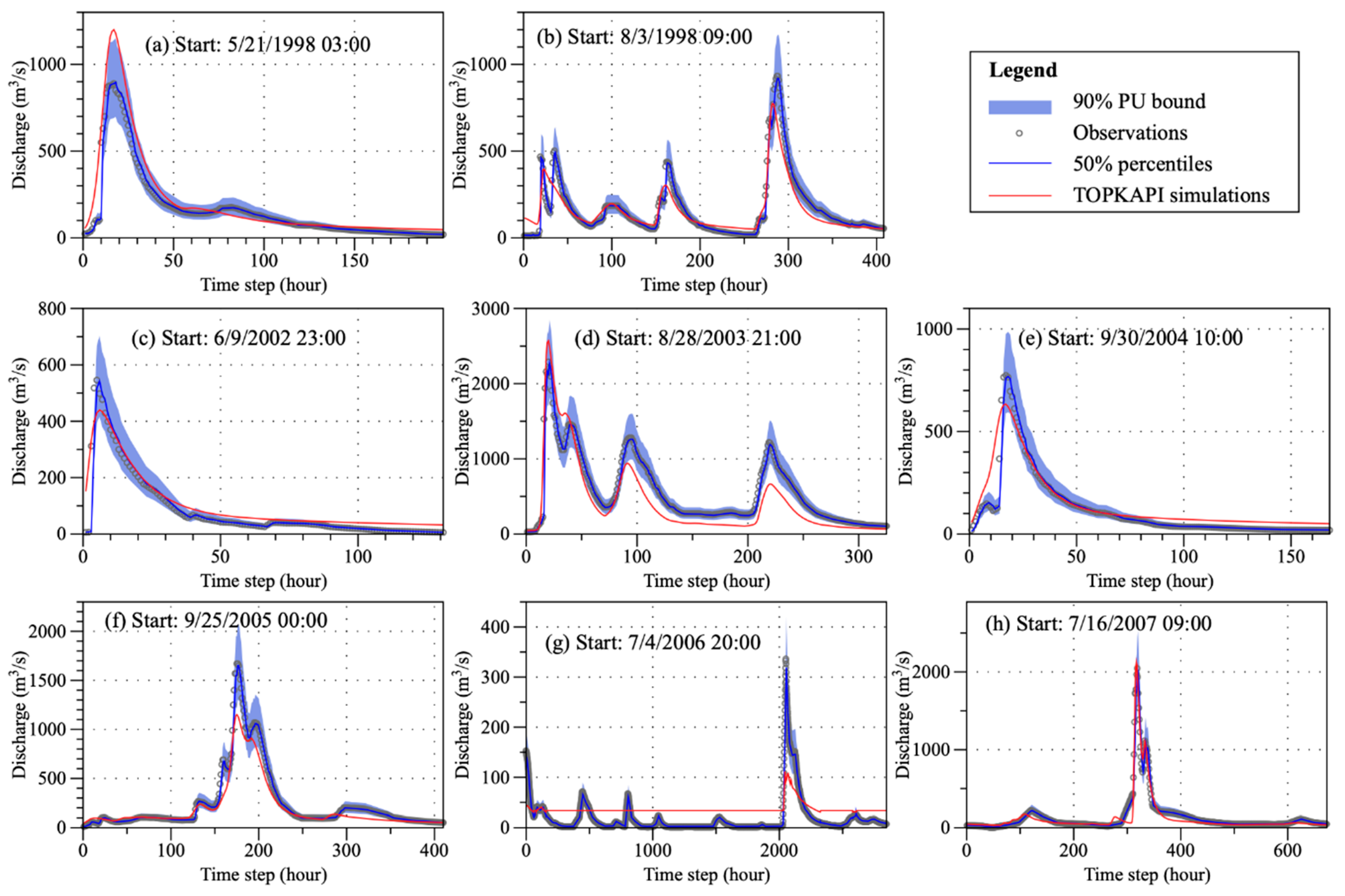
3.2. Flood Event Simulations

We also presented the model performance of eight flood events in Figure 6. The deterministic results of these flood events were produced by the TOPKAPI model as shown in Figure 4 and Figure 5. The HUP model was used to analyze the total forecast uncertainty of the deterministic results using the leading time of one hour. In the deterministic forecast results, the relative bias of flood peak (RBP) in five flood events satisfied the requirement of $\left|RBP\right|\le 20\%$, and the average absolute value of RBP in all eight floods was 25.4%. In terms of relative bias of flood volume (RBV), the simulation results of three floods satisfied the accuracy requirements ($\left|RBV\right|\le 20\%$), while the NSCE values of the selected flood events were greater than 0.75, except for the 2006 flood season.

The HUP provided the 90% PU bounds and 50% percentiles in the flood simulations, and the latter can be used as the deterministic results. The 50% percentiles simulations had very high accuracies in terms of the RBP and RBV indices. The absolute value of RBP was less than 6% for all floods, while the $\left|RBV\right|$ value was even less than 2%. Besides, the 50% percentiles of all flood events matched very well with observations with the NSCE values greater than 0.9. It was obvious that compared with the TOPKAPI model, the deterministic forecast result provided by the 50% percentiles had a significant improvement in accuracy. This was because the observations were also used in the calculation of the HUP model. The 90% PU bounds could also provide useful information for operational flood forecast practices. With the leading time of one hour, more than 95% of observations were contained within the 90% PU bounds for all flood events. The DI statistic ranged from 0.54 to 0.65 with an average of 0.61 among these floods. Overall, the HUP model could provide rich information of probabilistic forecasts at a given CI and even better deterministic results than distributed models in terms of the 50% percentiles. However, this does not mean that the HUP model could run independently, because its input includes the deterministic model’s results. The main characteristic of the HUP model is that it can further improve the resulted generated by the deterministic models.

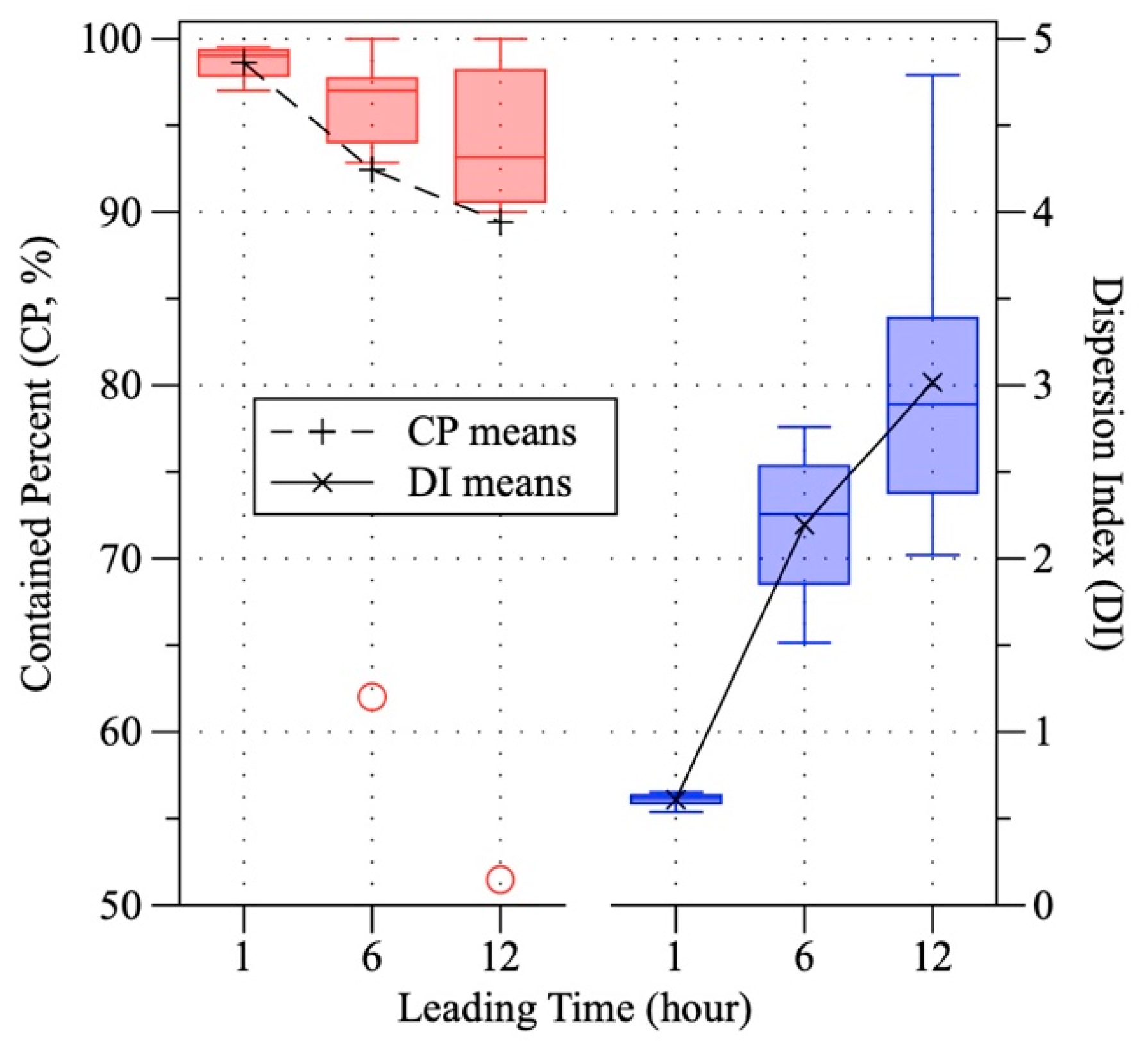
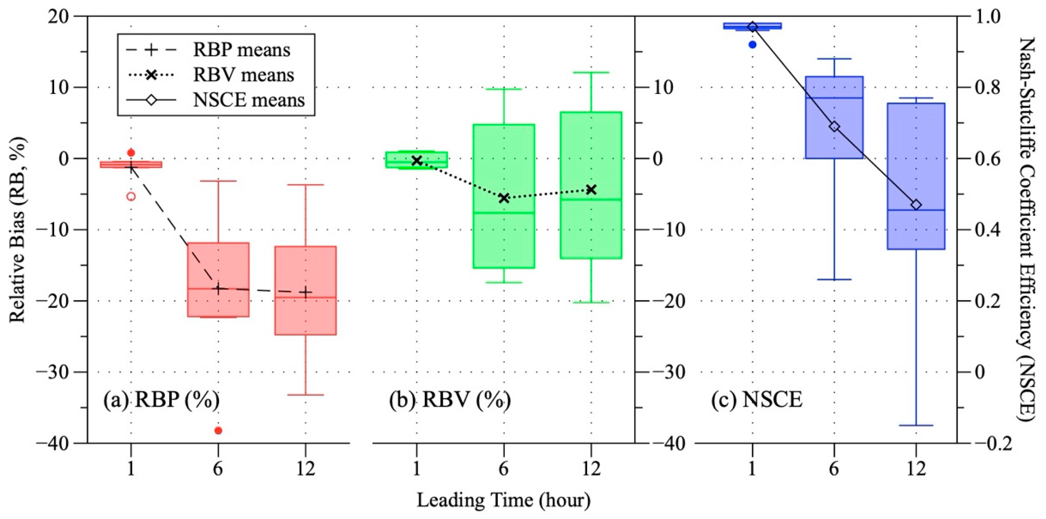
3.3. Model Accuracy Changes with Leading Time Increasing

The above comparison between TOPKAPI and HUP showed that the HUP model could provide very good agreement of hydrograph. Such a highly accurate result of the HUP model is essentially a real-time correction of flood forecasts using observed data. The leading time used by the HUP model was one hour. In operational practices, a one-hour leading time may not be sufficient for flood forecasts. Meanwhile, the observed discharge data may not be updated in time for use in the HUP model. Thus, large leading hours should be used. In this work, we conducted an analysis of HUP model accuracy changes with the increase in leading time (from one hour to six hours and to 12 h). Figure 7 shows the changes of the CP and DI statistics with the increase in leading time (1, 6 and 12 h). When the forecast leading time increased, the 90% PU bounds became wider than that of leading time = 1 h. That is to say, the DI value increased with the leading time. Although the 90% PU bounds had become wider, the number of observations enveloped by the bounds had decreased, manifested as a decrease in the CP value. The very low CP values (62% and 51%) could be found for the seventh flood event (June 2006) with the leading times of 6 and 12 h, respectively.

As the HUP model could also provide deterministic forecasts in terms of 50% percentiles of PU, the forecast accuracy of 50% percentiles of selected flood events was also analyzed at different leading times (Figure 8). All three performance indices showed a consistent decrease in accuracy as the forecast leading time increased. When the leading time increased from one hour to 6 h (or 12 h), the overall absolute values of the relative bias increased. Accordingly, the NSCE statistic decreased largely with the leading time increasing. Therefore, the accuracy of probabilistic flood forecasts provided by the HUP model decayed with the leading time increasing. This suggests that rolling forecasts with short leading times are very important not only in deterministic forecasts, but also in probabilistic forecasts.

4. Conclusions

Although many application cases of physically based distributed hydrological models have been reported in the literature, conceptual or lumped hydrological models are still the main ones in operational flood forecasting practices, especially in data-sparse regions. The main reason is that the quality of hydrometeorological or underlying data in many areas is low or even missing. In the localization of distributed models, therefore, large uncertainties are inevitably introduced to the final model forecasting results. In this study, we presented a case study of a distributed hydrological model (TOPKAPI) in flood forecasting with low-quality input data, and the forecast uncertainty was evaluated with a general uncertainty analysis framework (HUP model). In the study area (Lushi basin), the existing rainfall gauges cannot catch the spatial distribution of precipitation well. Rainfall estimates are easily overestimated or underestimated. Soil type data may also introduce uncertainties to the application of TOPKAPI as only eight FAO soil types are available. This number of soil types is not enough to describe the variability of soil characteristics in the study basin. In addition, observed discharge data are only available in the flood season. In operational flood forecasting practices, such uncertainties in TOPKAPI forecast results are very detrimental to flood control decisions. Therefore, probabilistic forecasting of the HUP model can provide new auxiliary information for flood prevention decisions.

The TOPKAPI model was calibrated using hourly hydrometeorological data (e.g., precipitation, air temperature and discharge) and underlying surface data (soil type and land use maps) for the period of 1996 to 2005, then the model was validated using date for the period 2006–2008. The average NSCE values for the calibration and validation were 0.78 and 0.82, respectively, and the average IOA values were 0.93 and 0.95, respectively. It was suggested that the overall model accuracy could be acceptable and the model generally reproduced the hydrological behaviors of the study basin. However, one can also see the low accuracy in some flood seasons, such as in the years 1997, 2001 and 2008. The HUP model was then used to output probabilistic forecasts for several flood events at different leading hours. At the leading time of one hour, the performance of deterministic forecasts provided by the 50% percentiles were largely improved with NSCE values greater than 0.9 for all flood events. Besides, more than 95% of observations were enveloped by the 90% PU bounds, and the average DI statistic was as small as 0.61 for all floods. This suggested that the HUP model could provide much information (both deterministic and probabilistic) for operational flood forecasting practices. In terms of both probabilistic (CP and DI) and deterministic (RBP, RBV and NSCE) performance indices, the accuracy of the HUP model at a leading time of 6 h or 12 h obviously decreased compared to that of leading time = one hour. This proved that the performance of HUP would decay with the leading time increasing. This study could provide a useful reference for operational flood forecasting practices when only low-quality data are available for physically based distributed hydrological models.

References

1. McKinnon, S. Remembering and forgetting 1974: The 2011 Brisbane floods and memories of an earlier disaster. Geogr. Res. 2019, 57, 204–214. [Google Scholar] [CrossRef]
2. Aerts, J.C.J.H.; Botzen, W.J.; Clarke, K.C.; Cutter, S.L.; Hall, J.W.; Merz, B.; Michel-Kerjan, E.; Mysiak, J.; Surminski, S.; Kunreuther, H. Integrating human behaviour dynamics into flood disaster risk assessment. Nat. Clim. Chang. 2018, 8, 193–199. [Google Scholar] [CrossRef] [Green Version]
3. Jongman, B.; Hochrainer-Stigler, S.; Feyen, L.; Aerts, J.C.J.H.; Mechler, R.; Botzen, W.J.W.; Bouwer, L.M.; Pflug, G.; Rojas, R.; Ward, P.J. Increasing stress on disaster-risk finance due to large floods. Nat. Clim. Chang. 2014, 4, 264–268. [Google Scholar] [CrossRef]
4. Vercruysse, K.; Dawson, D.A.; Glenis, V.; Bertsch, R.; Wright, N.; Kilsby, C. Developing spatial prioritization criteria for integrated urban flood management based on a source-to-impact flood analysis. J. Hydrol. 2019, 578, 124038. [Google Scholar] [CrossRef]
5. Li, B.; Yu, Z.; Liang, Z.; Acharya, K. Hydrologic response of a high altitude glacierized basin in the central Tibetan Plateau. Glob. Planet. Chang. 2014, 118, 69–84. [Google Scholar] [CrossRef]
6. Yu, M.; Li, Q.; Liu, X.; Zhang, J. Quantifying the effect on flood regime of land use pattern changes via hydrological simulation in the upper Huaihe River Basin, China. Nat. Hazards 2016, 84, 2279–2297. [Google Scholar] [CrossRef]
7. Liang, Z.; Tang, T.; Li, B.; Liu, T.; Wang, J.; Hu, Y. Long-term streamflow forecasting using SWAT through the integration of the random forests precipitation generator: Case study of Danjiangkou Reservoir. Hydrol. Res. 2018, 49, 1513–1527. [Google Scholar] [CrossRef] [Green Version]
8. Cloke, H.L.; Pappenberger, F. Ensemble flood forecasting: A review. J. Hydrol. 2009, 375, 613–626. [Google Scholar] [CrossRef]
9. Xiao, Z.; Liang, Z.; Li, B.; Hou, B.; Hu, Y.; Wang, J. New flood early warning and forecasting method based on similarity theory. J. Hydrol. Eng. 2019, 24, 04019023. [Google Scholar] [CrossRef] [Green Version]
10. Adnan, R.M.; Liang, Z.; Heddam, S.; Zounemat-Kermani, M.; Kisi, O.; Li, B. Least square support vector machine and multivariate adaptive regression splines for streamflow prediction in mountainous basin using hydro-meteorological data as inputs. J. Hydrol. 2020, 124371. [Google Scholar] [CrossRef]
11. Liang, Z.; Xiao, Z.; Wang, J.; Sun, L.; Li, B.; Hu, Y.; Wu, Y. An improved chaos similarity model for hydrological forecasting. J. Hydrol. 2019, 577, 123953. [Google Scholar] [CrossRef]
12. Belabid, N.; Zhao, F.; Brocca, L.; Huang, Y.; Tan, Y. Near-real-time flood forecasting based on satellite precipitation products. Remote Sens. 2019, 11, 252. [Google Scholar] [CrossRef] [Green Version]
13. Jiang, X.; Gupta, H.V.; Liang, Z.; Li, B. Toward improved probabilistic predictions for flood forecasts generated using deterministic models. Water Resour. Res. 2019, 55, 9519–9543. [Google Scholar] [CrossRef]
14. Todini, E. Hydrological catchment modelling: Past, present and future. Hydrol. Earth Syst. Sci. 2007, 11, 468–482. [Google Scholar] [CrossRef] [Green Version]
15. Bloschl, G.; Reszler, C.; Komma, J. A spatially distributed flash flood forecasting model. Environ. Model. Softw. 2008, 23, 464–478. [Google Scholar] [CrossRef]
16. Shafizadeh-Moghadam, H.; Valavi, R.; Shahabi, H.; Chapi, K.; Shirzadi, A. Novel forecasting approaches using combination of machine learning and statistical models for flood susceptibility mapping. J. Environ. Manag. 2018, 217, 1–11. [Google Scholar] [CrossRef] [Green Version]
17. Ritter, A.; Munoz-Carpena, R. Performance evaluation of hydrological models: Statistical significance for reducing subjectivity in goodness-of-fit assessments. J. Hydrol. 2013, 480, 33–45. [Google Scholar] [CrossRef]
18. Li, B.; Liang, Z.; He, Y.; Hu, L.; Zhao, W.; Acharya, K. Comparison of parameter uncertainty analysis techniques for a TOPMODEL application. Stoch. Environ. Res. Risk Assess. 2017, 31, 1045–1059. [Google Scholar] [CrossRef]
19. Li, B.; He, Y.; Ren, L. Multisource hydrologic modeling uncertainty analysis using the IBUNE framework in a humid catchment. Stoch. Environ. Res. Risk Assess. 2018, 32, 37–50. [Google Scholar] [CrossRef]
20. Huang, H.; Liang, Z.; Li, B.; Wang, D.; Hu, Y.; Li, Y. Combination of multiple data-driven models for the long-term monthly runoff predictions based on Bayesian Model Averaging. Water Resour. Manag. 2019, 33, 3321–3338. [Google Scholar] [CrossRef]
21. Liu, Z.; Martina, M.L.V.; Todini, E. Flood forecasting using a fully distributed model: Application of the TOPKAPI model to the Upper Xixian Catchment. Hydrol. Earth Syst. Sci. 2005, 9, 347–364. [Google Scholar] [CrossRef] [Green Version]
22. Li, D.; Liang, Z.; Li, B.; Lei, X.; Zhou, Y. Multi-objective calibration of MIKE SHE with SMAP soil moisture datasets. Hydrol. Res. 2019, 50, 644–654. [Google Scholar] [CrossRef] [Green Version]
23. Sun, W.; Wang, Y.; Wang, G.; Cui, X.; Yu, J.; Zuo, D.; Xu, Z. Physically based distributed hydrological model calibration based on a short period of streamflow data: Case studies in four Chinese basins. Hydrol. Earth Syst. Sci. 2017, 21, 251–265. [Google Scholar] [CrossRef] [Green Version]
24. Zhang, L.; Jin, X.; He, C.; Zhang, B.; Zhang, X.; Li, J.; Zhao, C.; Tian, J.; DeMarchi, C. Comparison of SWAT and DLBRM for hydrological modeling of a mountainous watershed in arid northwest China. J. Hydrol. Eng. 2016, 21, 04016007. [Google Scholar] [CrossRef]
25. Xu, H.; Xu, C.Y.; Chen, S.; Chen, H. Similarity and difference of global reanalysis datasets (WFD and APHRODITE) in driving lumped and distributed hydrological models in a humid region of China. J. Hydrol. 2016, 542, 343–356. [Google Scholar] [CrossRef]
26. Xu, B.; Boyce, S.E.; Zhang, Y.; Liu, Q.; Guo, L.; Zhong, P.-A. Stochastic programming with a joint chance constraint model for reservoir refill operation considering flood risk. J. Water Resour. Plan. Manag. 2017, 143, 04016067. [Google Scholar] [CrossRef]
27. Xu, B.; Zhu, F.; Zhong, P.-A.; Chen, J.; Liu, W.; Ma, Y.; Guo, L.; Deng, X. Identifying long-term effects of using hydropower to complement wind power uncertainty through stochastic programming. Appl. Energy 2019, 253, 113535. [Google Scholar] [CrossRef]
28. Chen, T.; Ren, L.; Yuan, F.; Yang, X.; Jiang, S.; Tang, T.; Liu, Y.; Zhao, C.; Zhang, L. Comparison of spatial interpolation schemes for rainfall data and application in hydrological modeling. Water 2017, 9, 342. [Google Scholar] [CrossRef] [Green Version]
29. Xu, W.; Zou, Y.; Zhang, G.; Linderman, M. A comparison among spatial interpolation techniques for daily rainfall data in Sichuan Province, China. Int. J. Climatol. 2015, 35, 898–2907. [Google Scholar] [CrossRef]
30. Wagner, P.D.; Fiener, P.; Wilken, F.; Kumar, S.; Schneider, K. Comparison and evaluation of spatial interpolation schemes for daily rainfall in data scarce regions. J. Hydrol. 2012, 464, 388–400. [Google Scholar] [CrossRef]
31. Huang, H.; Liang, Z.; Li, B.; Wang, D. A new spatial precipitation interpolation method based on the information diffusion principle. Stoch. Environ. Res. Risk Assess. 2019, 33, 765–777. [Google Scholar] [CrossRef]
32. De Amorim Borges, P.; Franke, J.; da Anunciação, Y.M.T.; Weiss, H.; Bernhofer, C. Comparison of spatial interpolation methods for the estimation of precipitation distribution in Distrito Federal, Brazil. Theor. Appl. Climatol. 2016, 123, 335–348. [Google Scholar] [CrossRef]
33. Li, B.; Liang, Z.; Bao, Z.; Wang, J.; Hu, Y. Changes in streamflow and sediment for a planned large reservoir in the middle Yellow River. Land Degrad. Dev. 2019, 30, 878–893. [Google Scholar] [CrossRef] [Green Version]
34. Ciarrapica, L. Topkapi: A New Approach to Rainfall-Runoff Modelling. Ph.D. Thesis, University of Bologna, Bologna, Italy, 1995. [Google Scholar]
35. Liu, Z. Toward a Comprehensive Distributed/Lumped Rainfall-Runoff Model: Analysis of Available Physically-Based Models and Proposal of a New TOPKAPI Model. Ph.D. Thesis, University of Bologna, Bologna, Italy, 2002. [Google Scholar]
36. Abbott, M.B.; Bathurst, J.C.; Cunge, J.A.; O’Connell, P.E.; Rasmussen, J. An introduction to the European hydrological system—Systeme hydrologique Europeen, “SHE”, 1: History and philosophy of a physically-based, distributed modelling system. J. Hydrol. 1986, 87, 45–59. [Google Scholar] [CrossRef]
37. Abbott, M.B.; Bathurst, J.C.; Cunge, J.A.; O’Connell, P.E.; Rasmussen, J. An introduction to the European hydrological system—Systeme hydrologique Europeen, “SHE”, 2: Structure of a physically-based, distributed modelling system. J. Hydrol. 1986, 87, 61–77. [Google Scholar] [CrossRef]
38. Thornthwaite, C.W. An approach toward a rational classification of climate. Geogr. Rev. 1948, 38, 55–94. [Google Scholar] [CrossRef]
39. Krzysztofowicz, R. Bayesian theory of probabilistic forecasting via deterministic hydrological model. Water Resour. Res. 1999, 35, 2739–2750. [Google Scholar] [CrossRef] [Green Version]
40. Biondi, D.; De Luca, D.L. Performance assessment of a Bayesian forecasting system (BFS) for real-time flood forecasting. J. Hydrol. 2013, 479, 51–63. [Google Scholar] [CrossRef]
41. Li, B.; Liang, Z.; Zhang, J.; Chen, X.; Jiang, X.; Wang, J.; Hu, Y. Risk analysis of reservoir flood routing calculation based on inflow forecast uncertainty. Water 2016, 8, 486. [Google Scholar] [CrossRef]
42. Liu, Z.; Guo, S.; Xiong, L.; Xu, C.Y. Hydrologic uncertainty processor based on a copula function. Hydrol. Sci. J. 2017, 63, 74–86. [Google Scholar] [CrossRef]
43. Han, S.; Coulibaly, P. Probabilistic flood forecasting using hydrologic uncertainty processor with ensemble weather forecasts. J. Hydrometeorol. 2019, 20, 1379–1398. [Google Scholar] [CrossRef]
44. Yao, Y.; Liang, Z.; Zhao, W.; Jiang, X.; Li, B. Performance assessment of hydrologic uncertainty processor through the integration of the principal components analysis. J. Water Clim. Chang. 2019, 10, 379–390. [Google Scholar] [CrossRef]
45. Feng, K.; Zhou, J.; Liu, Y.; Lu, C.; He, Z. Hydrologic uncertainty processor (HUP) with estimation of the marginal distribution by a Gaussian mixture model. Water Resour. Manag. 2019, 33, 2975–2990. [Google Scholar] [CrossRef]
46. Krzysztofowicz, R.; Kelly, K.S. Hydrologic uncertainty processor for probabilistic river stage forecasting. Water Resour. Res. 2000, 36, 3265–3277. [Google Scholar] [CrossRef]
Figure 1. The drainage catchment above the Lushi hydrological station.
Sustainability 12 08268 g001
Figure 2. The land use and soil type maps of the Lushi basin.
Sustainability 12 08268 g002
Figure 3. Flowchart of the TOPographic Kinematic Approximation and Integration (TOPKAPI) model.
Sustainability 12 08268 g003
Figure 4. Calculated and measured hourly discharge time series at the Lushi station for the calibration period: (a) 1996–2000, and (b) 2001–2005.
Sustainability 12 08268 g004
Figure 5. Same as Figure 4 but for the validation period 2006–2008.
Sustainability 12 08268 g005
Figure 6. Flood hydrograph comparisons of observations, deterministic results (with TOPKAPI simulations) and probabilistic results (with HUP model at the leading time of one hour).
Sustainability 12 08268 g006
Figure 7. Changes in the Contained Percent (CP) and Dispersion Index (DI) statistics with the increase in forecast leading time for the selected eight flood events in the Lushi basin.
Sustainability 12 08268 g007
Figure 8. Changes in the relative bias of flood peak (RBP), relative bias of flood volume (RBV) and Nash–Sutcliffe Coefficient Efficiency (NSCE) with the increase of forecast leading time for the selected eight flood events in the Lushi basin.
Sustainability 12 08268 g008