Article

Towards Sustainable Cities: Utilizing Floating Car Data to Support Location-Based Road Network Performance Measurements

Faculty of Business, Economics and Management Information Systems, University of Regensburg, Universitätsstraße 31, 93053 Regensburg, Germany
*
Author to whom correspondence should be addressed.
Sustainability 2020, 12(19), 8145; https://doi.org/10.3390/su12198145
Submission received: 25 August 2020 / Revised: 24 September 2020 / Accepted: 28 September 2020 / Published: 2 October 2020
(This article belongs to the Special Issue Sustainable Operations and Logistics)

Abstract

:
Road network performance (RNP) is a key element for urban sustainability as it has a significant impact on economy, environment, and society. Poor RNP can lead to traffic congestion, which can lead to higher transportation costs, more pollution and health issues regarding the urban population. To evaluate the effects of the RNP, the involved stakeholders need a real-world data base to work with. This paper develops a data collection approach to enable location-based RNP analysis using publicly available traffic information. Therefore, we use reachable range requests implemented by navigation service providers to retrieve travel times, travel speeds, and traffic conditions. To demonstrate the practicability of the proposed methodology, a comparison of four German cities is made, considering the network characteristics with respect to detours, infrastructure, and traffic congestion. The results are combined with cost rates to compare the economical dimension of sustainability of the chosen cities. Our results show that digitization eases the assessment of traffic data and that a combination of several indicators must be considered depending on the relevant sustainability dimension decisions are made from.

1. Introduction

Rising urbanization around the globe leads to high requirements in terms of urban sustainability [1]. Therefore, indicators to measure urban sustainability are an extensively discussed topic in literature [2,3,4,5]. These indicators often contain terms such as “mobility” [6], “efficient transportation”, or “transportation and roads” [7]. When dealing with the sustainability of transportation and the efficient movement of people and goods, in addition to topics such as railways [8] and public transportation [9,10,11,12,13], the urban road network is a major research area [14,15,16,17,18,19,20]. This stems from the fact that road network performance (RNP) can lead to significant negative impacts on all three dimensions of urban sustainability.
Economic sustainability can suffer in several ways. Many authors found that poor RNP, in terms of traffic congestion, is a reason for higher costs and reduces efficiency significantly [21,22,23,24,25,26]. In addition to that, traffic congestion intensified in the past [27,28], causing as much as 23 percent of all truck transportation delays [29].
Environmental sustainability is mainly focused on pollution and greenhouse gas emissions. A lot of literature proves the relation between traffic congestion and air pollution [30,31,32,33,34]. Longer travel distances and congestion lead to more pollution and a lower level of sustainability.
Social sustainability focuses on the well-being of the population. Poor RNP can lead to several health issues. Traffic congestion implies a higher number of vehicles polluting engine noises on road. The generated noise has a significant health impact [35,36] such as sleep disturbance and anxiety [37]. In addition to that, the number of accidents happening can depend on the road network [38,39,40].
RNP in general has been studied extensively over the years, employing different methods and geared towards different purposes [41,42,43,44,45]. Especially the relation between the three-dimensional urban sustainability (economy, environment, and society) and the road network has been addressed.
An extensive body of literature discusses the reduction in traffic congestion [46,47,48]. Russo and Comi [49] analyze the effects of logistics measures on the economy of the city, Baghestani et al., Armah et al., Borza et al. and Zhang et al. [32,50,51,52] deal with on-road emissions and Kleiziené et al., Ohiduzzaman et al. and Sirin [36,37,53] discuss vehicle noise reduction and the development of quieter pavements.
To carry out these analyses, all stakeholders who are dealing with road networks and urban sustainability must gather a real-world data base to work with. Therefore, the research hypothesis of this paper can be formulated as follows:
How can relevant data be collected programmatically to measure road network performance?
The long-term trend towards digitizing the environment, including the logistical infrastructure such as road networks and vehicles, fundamentally eases the programmatical assessment of information and gives way to study new data collection methods [54,55,56,57]. Due to this, the purpose of this paper is to develop a new methodological approach to gather relevant RNP data on an area-wide scale. An exemplary application of the gathered data on the economic dimension is demonstrated on four selected cities in Germany to prove the usability of the proposed methodology. Thus, the paper deals with what Sun et al. [58] call the physical issues of RNP, i.e., we are concerned with the determination of travel times, travel speed, and traffic conditions.
The paper is organized as follows: Section 2 provides theoretical information on RNP measurement and the underlying data collection procedure. In Section 3, a data collection method for measuring RNP is presented by providing an exemplary use case. In Section 4, this methodology is applied to four German cities and a comparison of these cities is carried out. In Section 5, theoretical and practical implications are discussed. An outlook for further research is provided in Section 6, followed by a short conclusion highlighting the main takeaways of this paper.

2. Literature Review

2.1. Fundamentals on Road Network Performance Measurements

The assessment of RNP has been widely researched. We start by introducing our definition and will then give reference to the extant body of research. We suggest defining RNP generally as the network driven impact on sustainability. In the context of this paper, we particularly focus on the economic dimension, which leads to the refined definition of RNP as being the network driven economical costs of moving a vehicle from a specified origin to a specified destination using the road network. Although the definition is open, we confine our analysis to urban transportation, i.e., short distance traffic, sometimes called the last mile or urban cargo traffic [59,60]. The road network is defined as the set of roads that can be used by vehicles. Thus, our definition of RNP is geared towards the structural properties of the network that shapes the flows within the network and affects operational performance [61,62]. The definition acknowledges but excludes the analysis of further notions or indicators of network performance, such as levels of service, capacity, safety, smoothness of flow, reliability, vulnerability, accessibility, resource constraints, or travel time reliability [63], that, respectively, represent the functionality of the network for particular research goals. As our analysis is restricted to network driven costs only, it is confined to a share of the total cost only. The cost of moving a vehicle is determined by many factors such as vehicle type [64], toll [65] or fuel [66]. We restrict the analysis to those factors that are related to the road network. The definition of RNP borrows in part from Santosa and Joewono [67] who measure RNP by speed and vehicle cost.
We suggest measuring RNP by detour and travel speed. Detour is defined as “road distance from origin to destination” over “aerial distance from origin to destination” [68]. Thus, detour represents widely discussed network attributes such as density [62] or connectivity [69]. Travel speed is defined as the average speed that can be driven from origin to destination considering vehicle and road constraints. Thus, travel speed summarizes road network attributes such as speed limits, traffic lights, or the level of congestion within the network [70,71,72]. Travel speed can be easily converted into travel time [73]. Thoen et al. [74] demonstrate that longer travel times lead to higher transportation costs, emphasizing the importance of determining travel times objectively.
Road distance is defined as the distance of a tour. A tour is defined as the network path a rational decision maker would choose to minimize the travel time from origin to destination. Thus, we assume an efficient use of existing road infrastructure and available traffic status information [75]. We suggest measuring RNP with reference to two factors only and thus depart from earlier approaches that suggest multi-criteria measurements such as Fancello et al. [42].
RNP results vary by tour since characteristics of the road network vary across space. Ciscal-Terry et al. [76] called this the origin-destination-distribution problem. Thus, a meaningful RNP statement must be specific on how to select the locations that enter the analysis.
Fundamentally, RNP can be measured via three origin-destination settings. One is to measure across the complete network, i.e., from anywhere to anywhere. A second setting measures from defined origins to defined destinations [77], i.e., from somewhere to somewhere. We suggest following a third setting, given an origin, we do not specify a destination and then measure detour and travel speed for the origin-destination pair but specify the origin only and list all destinations that can be reached within a given range or time frame.
Since we focus on studying RNP for general cargo moving purposes, typical logistics service providers’ locations such as freight transport centers, logistic zones or urban consolidation centers represent meaningful origins. For a case-specific analysis, Alho A.R. et al. [78] find that declared data regarding bases might not be as accurate as inferred data, suggesting the identification of central network nodes via algorithms instead of relying on survey data to determine meaningful points of origin. Referring to Saedi et al. [63] our approach does not report RNP across the complete road network but well-defined partitions.

2.2. Road Network Data Collection: Developing A New Method

Data sources to compute RNP have been mentioned in recent literature but have never been an explicit focus of the research community. Some papers model the variability of RNP via a stochastic framework and compute journey time estimators [79]. Figliozzi [22] uses tour data reported in the literature to perform a sensitivity analysis on changes in travel time and tour characteristics. The problem with this procedure is the availability of data as the current literature does not provide suitable or publicly available tour data for most areas around the world. Another way to gather road data is the usage of equipped single cars [80,81]. These cars are equipped with a range of sensors to record road data while driving. The extensive manpower and machinery required for this solution is multiplied as global coverage is attempted. Urban areas could be analyzed under consideration of induction loops, cameras, and sensors measuring current road traffic [82,83]. Data accessibility as well as processing data from a lot of different sources drive complexity of this data collection method. Mondschein and Taylor [21] interviewed people about personal trip data and corresponding travel times. Two major concerns arise when we take a closer look at this procedure. Global coverage is very weak as a lot of interviews must be conducted to gather enough data for one specific area. An additional problem are people’s privacy concerns when sharing their driving data [22]. A “digital version” of interviewing people is the usage of navigation service providers’ application programming interfaces (APIs) as these providers gather and compress anonymized data from all their users [84]. The anonymization of data also overcomes the privacy concerns mentioned before. Kellner et al. [77] used navigation service providers’ data to build distance matrices with customers’ locations and requested travel times at different times throughout the day. To generalize the approach by Kellner et al. [77] and bypass any problems related to subjective trip generation, as for example experienced by Sun et al. [85], we use real-world floating car data (FCD) with compressed information collected over time.
The use of FCD to evaluate traffic status has been studied intensively [86,87,88,89,90,91,92]. However, there is no research that exploits FCD, especially FCD processed into reachable ranges, to assess RNP. That is what we suggest doing.
Processing FCD to measure RNP is challenging as traffic data can be considered big data due to its complexity and heterogeneity [78,93,94]. However, navigation service providers can produce the needed data efficiently [84]. Due to this, we suggest using navigation service providers’ APIs, especially retrieving so-called “reachable ranges”.
A “reachable range” is defined as an area that can be reached by a specific vehicle under certain constraints such as maximum travel time or maximum travel distance starting at a specified location. The use of reachable ranges to assess networks has gained only limited attention so far. Hirako et al. [95] analyze reachable areas to understand the travel behavior of elderly citizens to medical facilities. Referring to Phan et al. [96], calculating a reachable range is one part of the algorithm for maximizing range sum queries turned inside out.
In our case, we retrieve a reachable set K c that consists of 50 nodes that can be reached from origin node v 0 by the end of constraint c [97]. As a result, we obtain a subgraph showing only one origin and 50 reachable destinations. Assuming a completely paved environment, the reachable range would resemble a circle. In a real-world scenario, it will be a snowflake-shaped object with some locations being closer to the origin (areas with poor RPN) and some locations further from the origin (areas with good RNP).
By combining this information with the need for multi-time measurements, we obtain time-dependent graphs. By varying the defined timeframe, the RNP measurement can be suited to different goals of the analysis.
Our approach is considered efficient as wide areas can be analyzed by a few API calls. This allows measuring RNP on a large scale for defined origins without the need for second best solutions such as regional aggregation as suggested by Casadei et al. [98] for instance.

3. Methodology

3.1. Basic Idea

To measure RNP and make regional comparisons using speed information, the following data are required: free flow and congested speeds, which can be derived from travel times and travel distances as well asair distances, which in relation to previously determined actual road travel distances enable a detour calculation.
To investigate the relation between the time of day and congestion-induced delays, exemplary trips are simulated leading from the city center outwards (to the east, west, north and south) for every city considered in the comparison below (Section 4). The results generated via the TomTom routing API are shown in Figure 1. From 03:40 to 21:50 delays are occurring in every city. Two rush hours can be identified, the first one can be classified as the morning rush hour where large numbers of employees commute to work and more than 75 percent of commercial distribution tours depart from their origin as observed by Nuzzolo et al. [99]. It peaks at about 08:00, in accordance with the observations made in Italy. The second rush hour peaks at 17:00, when most people are heading home from work. In between these rush hours the congestion-induced delays settle in Hamburg, Munich and Stuttgart whereas Berlin shows a rise in level of delay until peak rush hour is reached. The interval from 22:00 to 03:30 the next day can be considered as free flow state as there are no congestion-induced delays measured.
The data collection process uses the TomTom reachable range API. It returns the reachable area in the form of reachable destinations from a certain starting point in the form of a polygon. The restrictions for the reachability analysis can be as follows: maximum travel distance = “distance budget”, maximum travel time = “time budget”, or maximum fuel consumption = “fuel budget”.
This API has become more and more interesting, especially during the electrification of vehicles because it is possible to determine which locations can be reached with a given battery capacity and a corresponding consumption.
In the context presented in this paper, the API is used to determine all locations that can be reached within a time or distance restriction. Many parameters can be specified as input variables. The most important parameters in this context are shown in Table 1 below:
As a result, the API always provides a polygon with a maximum of 50 corner points (see Figure 2), regardless of the selected input parameters. The area described by the polygon includes all geolocations that can be reached considering the specified restrictions. For each corner point of the polygon, the corresponding air distance can be estimated using the great circle distance formula [100]. Consequently, the air distance can be used as a common base to compare queries for different restriction parameters.
The data collection methodology to determine the attributes detour factor, infrastructure and traffic congestion is explained below. The parameters Origin, Travel Mode and Route Type are identical for all queries. In case of the following example, the starting point “Schäftlarnstraße 10, 81371 Munich, Germany” with the coordinates of 48.116431 degrees latitude and 11.556811 degrees longitude is selected. The parameter Travel Mode is set to “truck”, the Route Type requested is “fastest”.
To summarize the data collection methodology, necessary variables are defined in Table 2. All three calculation steps are presented in Table 3 and explained in depth in the following sections.
The next subsections focus on an in-depth explanation of the collection methodology to understand the requirements and results of every step. In addition, the generated data are visualized by individual charts. Connections between marks within one chart indicate that the gradients are results of continuous regressions based on discrete measures.

3.2. Detour

Detour in general is defined as the difference between travel distance via road and the corresponding air distance. The detour factor is defined as the quotient of travel distance and calculated air distance between two points. It will always be greater-than or equal to 1.0, because the shortest travel distance is always a straight line and thus equals the air distance. The detour factor changes with the length of the travel distance/air distance (with increasing air distance, straight routes such as highways can be used, which reduces the detour factor). However, the API query only accepts one maximum travel distance value as a restriction at a time. Consequently, one query for each value between 1 km and 30 km travel distance (= distance budget) with a step size of 1 km is requested and the returned polygons analyzed. The parameter Depart At is not relevant here as the polygon is calculated via a traffic-independent shortest path algorithm.
In the last step, the query’s restriction (= travel distance) can be related to the average value of the calculated air distances. Thus, for each travel distance a corresponding air distance and a detour factor is calculated. The relationship between air distance and detour factor can be displayed using a polynomial regression. In our example, this results in the chart shown in Figure 3:
One can clearly see that the detour factor decreases with increasing air distance, which is due to the possibility of using relatively straight routes (e.g., access to inner-city highways or the German motorway network), until it reaches a nearly stable value (in this case about 1.5).

3.3. Infrastructure

After determining the detour factor regression, the API can be used to determine the average speed during free-flow state. The free-flow state describes the traffic flow without congestion exceeding an agreed upon norm [101]. This means that delays due to infrastructural influences such as speed limits or traffic light changes are considered part of the free flow. Consequently, the average free-flow speed provides a quantification of the existing infrastructure. In order to determine this average speed, queries are formulated sequentially to retrieve points that can be reached for a certain journey duration. For this purpose, the queries are restricted by applying a time budget restriction. To ensure free-flow conditions, the parameter Depart At is set to 00:00:00. This time is derived from Figure 1 as there is no delay measured in any of the investigated regions. Using the returned polygon, the average air distance between all polygon corners and the starting point can be calculated per iteration step. The time steps and their corresponding free flow distances are shown in Figure 4. However, the magnitude of the travel distance is dependent on the air distance and implicitly manipulated via the detour factor. For this reason, a travel distance is estimated using air distance averages and the corresponding detour factor, as is shown by the formula in Table 3. The ratio of travel distance to travel time returns the average free flow travel speed.

3.4. Traffic Congestion

With the given definition of free-flow state in mind, the effect of traffic congestion can be measured by the difference between free-flow speed and congested speed. The travel speed in congested state can be determined by repeating the procedure for calculating the free-flow speed, setting the Depart At parameter at a time suitable for the analyzed scenario. In the context of this research, we set the Depart At parameter of the API query to 07:00:00. The results are shown in Figure 5. The ratio of travel distance (estimated by using the detour factor regression) to travel time again gives the average travel speed.

3.5. Speed Comparison

To compare free flow and congested states more clearly, Figure 6 shows the average travel speed as a function of the travel distance for both states of the road network. By using a power regression model of the free flow and congested speeds, the speed difference can be determined continuously throughout the analyzed travel distance interval.
Both speed profile curves displayed in Figure 6 clearly show a degressive course. When reaching beyond the localized, urban space, both slopes approach a common value. The convergence of these curves can be explained as follows: as the travel distance increases, the traffic density usually decreases outside the inner-city boundaries and traffic volume considered with the API-calls corresponds more and more to the free flow state. The actual value that both graphs converge towards can be explained by referring to the route type, which is defined as fastest for all calls. This means that roads with the highest possible travel speed (usually motorways) are favored for the analysis. Consequently, the asymptote of the two speed graphs corresponds to the average speed at which the vehicle type defined in travel mode moves on motorways.

3.6. Area Comparison

Travel times needed to reach an end point from a start point are the result of travel distance and travel speed of the specific route. To compare different areas, a combination of detour based on the street layout and delays based on traffic influences must be considered. This means that both the detour and traffic factor for different areas must be calculated based on a comparable variable. Since in practice, the determination of air distances with the help of the great circle formula is easy to implement and free of location-specific influences, the air distance is chosen as the comparable variable. The goal of this area comparison is to derive a travel distance and travel time for free and congested states depending on the covered air distance. The travel distance on the one hand can already be determined by the air distance multiplied with the detour factor: d t = d a d f d a . On the other hand, the travel time is calculated as follows: t t = d a d f d a v   d a . The travel time comparison is shown in Figure 7.
The combination of travel distance per air distance and travel time per air distance allows us to assess the considered area based on sustainability aspects. To show the applicability of our measures in the context of sustainability we focus on analyzing one specific sustainability dimension: the economical sustainability is measured by costs per air distance. Therefore, we assume EUR 0.7 per kilometer driving costs, an hourly wage of EUR 20.5 as driver costs and EUR 7.5 per hour of vehicle occupation costs, which is in line with other literature [102]. Continuing, the costs per air distance kilometer for Munich are shown individually and in total in Figure 8.
All curves are degressive. The costs during free flow (dashed lines) are always slightly below the congested graphs, although they become more and more similar over time due to the aforementioned reason of motorway access when the air distance increases. The relationship between driving costs and the combination of driver plus vehicle occupation costs is particularly noteworthy. With increasing distance, the driver and vehicle occupation costs are dominated by the driving costs. In this example, the driving costs exceed the driver and vehicle occupation costs in free flow/in the congested state from 8/12 air kilometers. On average, the congested mode results in higher costs of about 12 cents per air distance kilometer compared to free flow, which corresponds to additional costs of about 6.7%.

4. Case Study: Comparison of Four German Cities by Detour, Infrastructure and Traffic Congestion Indices and Their Impact on Road Network Performance
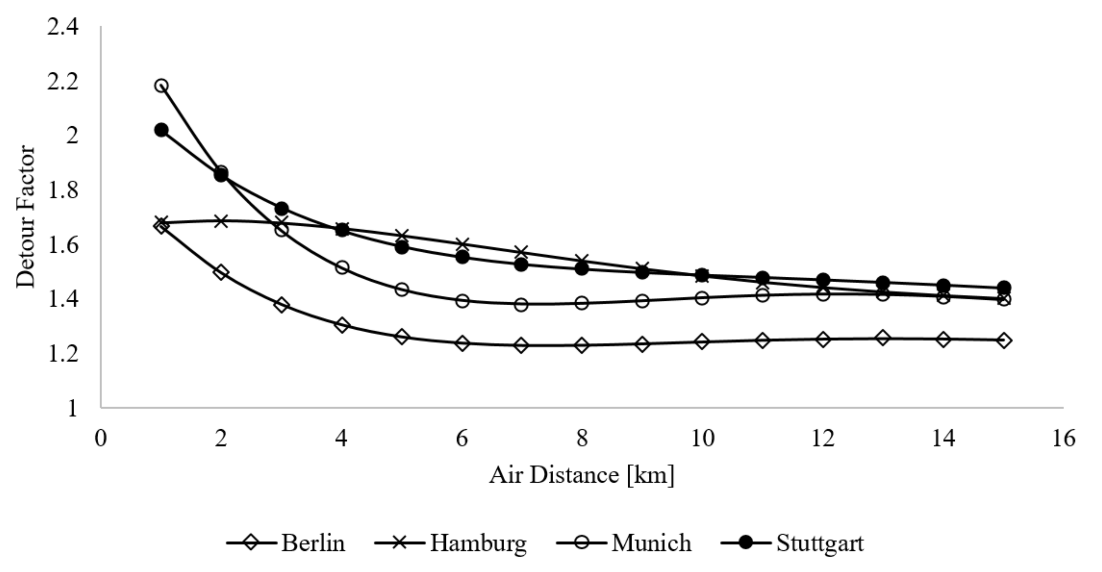
In order to compare four different cities, data on detour factor, travel speed, and costs are determined in free flow and congested states for each city using the previously described methodology. The four selected cities are Berlin, Hamburg, Munich, and Stuttgart as they are ranked among the top six German cities within the 2019 TomTom traffic index ranking. The central starting locations shown in Table 4, mainly based on existing depots by local transportation service providers, were used in this case study:
In the following paragraphs, all results are plotted and interpreted. In the descriptions of the diagrams, the keyword “collected” indicates that the data shown are displayed as it has been retrieved and has not been smoothed or modified in any way. “Calculated” means that the data were estimated by regression and therefore smoothing can occur. The curves of the different cities are always marked identically to allow for easy comparison as shown in Figure 9:

4.1. Detour Factor

The detour factors in Figure 10 describe the interaction between air distance, street network density, and straightforwardness of existing connections. By taking a closer look at the curves of the detour factors, it is noticeable that the detour factors of the three cities Hamburg, Munich, and Stuttgart develop nearly identically, starting at about 11 km air distance and approach a value of 1.4. In addition, the course of the curve for Hamburg is noteworthy, as it is rather constant at the beginning in contrast to the other curves. This indicates a strong deviation from a road network made up of straight connections around the centralized starting point, which is the case in Hamburg due to the river Elbe and its many waterways inside the inner-city area. Only after exiting the inner-city area and gaining motorway access, the detour factor decreases as more direct connections become available. Lastly, Berlin’s detour factor is consistently lower than all other detour factors, which indicates a well-developed road network.

4.2. Travel Times

The travel time curves provide information on how cities position in terms of infrastructure and congestion measurement. Four different charts are generated. The two charts in Figure 11 show the travel distance in relation to the travel time both in free flow and congested states. The next two charts in Figure 12 focus on travel distance loss. The left chart in Figure 12 shows the absolute difference between these curves. The right chart shows the relative loss of travel distance from free flow to congested status.
It is apparent that Stuttgart has the highest travel distances compared to the given travel times in both free flow and congested states. When looking at the relative loss curve for Stuttgart, we notice that it is relatively low compared to the other curves. This means that Stuttgart does not have a major congestion problem and the city has a very good infrastructure.
The counterexample to this is Hamburg. The speed of movement tends to be lowest in Hamburg in free flow and congested states. The relative loss curve for Hamburg is above average. This suggests a poor infrastructure, as the possible travel distances without traffic are already relatively low. The congested state in Hamburg can be classified as slightly above average in comparison.
The most congested cities are Munich and Berlin, with Berlin showing a relatively constant relative loss of around 16 percent (0.16) compared to free flow. Munich, on the other hand, is characterized by an increasing level of relative loss, which is approaching 17 percent (0.17).
Depending on the observation interval, Berlin (up to 10 min of travel time) or Munich (from 10 min of travel time) can be classified as the most congested city in the comparison at 07:00:00 departure time.

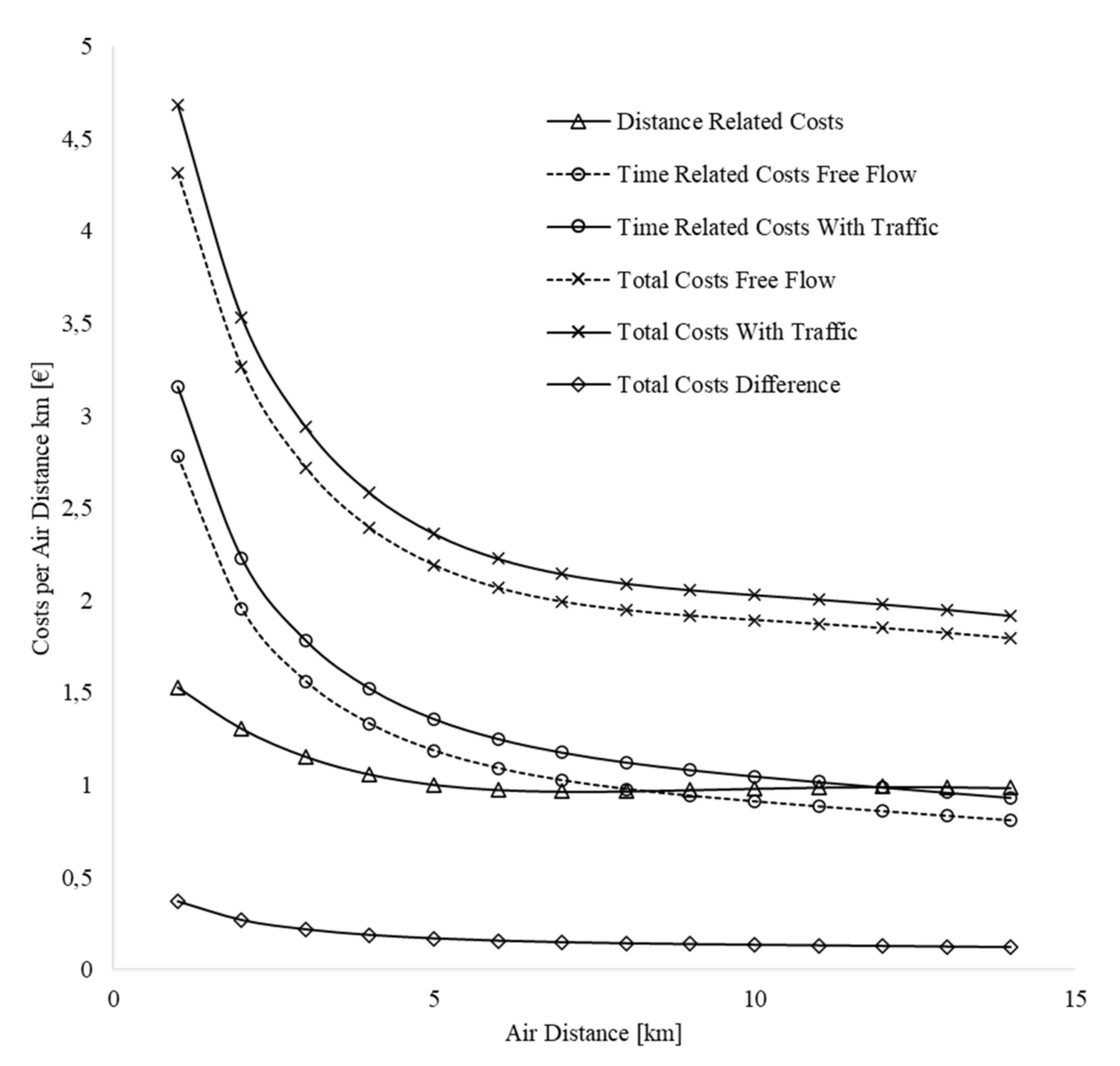
4.3. Transportation Costs

The economical sustainability of infrastructure, congestion and detour factor is reflected in total costs of transport. The cost rates from Section 3 were used for this calculation. The first two curves from left to right shown in Figure 13 represent costs per air distance kilometer for free flow and congested conditions. The right curve in Figure 13 shows the cost difference between congested and free flow.
The costs per kilometer are highest in both free flow and congested conditions in Hamburg. This can be explained by the fact that Hamburg has an average detour factor, a poor infrastructure, and a moderate traffic congestion level. Due to the average detour factor, the driving costs per air distance are also average, whereas the driver and vehicle occupation costs are far above average due to the low absolute speeds.
The graphs for Stuttgart in free flow and congested states are slightly above the curves of Munich and Berlin, which describe a comparable course. The absolute speeds are highest in Stuttgart, which means that the higher costs can only be explained by the higher detour factor of Stuttgart. Stuttgart’s detour curve is always above average and to a large extent the highest amongst all cities.
Munich and Berlin share the lowest costs per air distance kilometer. In Munich, the absolute speed is higher than in Berlin, both in free flow and congested states, with Berlin having a significantly lower detour factor. These two facts cancel each other out, resulting in both cities having an almost identical level of transport cost.
The cost difference curves allow conclusions to be drawn as to how much additional cost per air distance kilometer is incurred depending on the choice of departure time. In Berlin, different departure times cause the highest difference, Stuttgart the least and Hamburg and Munich show almost identical cost difference curves. In addition, the costs induced by congestion can vary between EUR 0.07 and EUR 0.5 per air distance kilometer, depending on the distance and city, which results in a considerable total cost difference for a high number of kilometers travelled.

4.4. City Comparison

When approaching a comparison of two or more regions from a RNP standpoint it is essential to define the scope of comparison. As we can derive from the subsections above it is not enough to know detour/travel speeds to conclude a transport cost related order of different regions. To order regions within the context of RNP, a clear perspective to interpret the data must be set. This perspective consists of the following three characteristics: (1) performance indicator; (2) daytime; and (3) air distance. To begin analyzing our four regions, one of the suggested (1) performance indicators must be chosen. This stems from the fact that analyzing only one regional performance indicator indicates high costs per kilometer but at the same time another performance indicator value compensates the first one and leads to lower costs per kilometer as we would have expected. For example, Stuttgart has a high detour factor, which—considered isolated—would lead to the expectation of high costs per kilometer. Stuttgart’s high travel speeds in contrast lead to low travel times and therefore result in transportation costs per kilometer being only slightly above average. Due to this, the interpretation of the level of different performance indicators must not be mixed up. Following that, a (2) daytime to compare regions must be set. This is of course necessary due to the fact that the level of traffic congestion and thus congested speeds/costs in congested state are highly time dependent as shown in Figure 1. As the peak congestion times are slightly different for specific regions the decision must be made whether different regions are analyzed at different times or whether one daytime for all regions is set. Individual daytimes for every region would allow comparison of peak congestion states whereas an identical starting time for every region increases comparability in cases where departure times are fixed (e.g., due to business and delivery hours/time windows). The last aspect to take care of is the air distance (3). Performance indicator values are dependent on the travelled air distance. Therefore, specific air distance intervals or fixed air distance values should be set to ensure context-specific analysis. To remotely compare regions without any knowledge about locations to be approached from the starting point, an average air distance of potential trips should be estimated. If precise information about locations to be approached is available, the distances between these locations and the starting point should be calculated and used for further analysis.

5. Discussion

The collection method presented in this paper assumes that the free flow condition in a traffic area occurs at midnight. This means that the time of departure influences the volume of traffic and thus the transportation costs incurred. To minimize these costs, the additional costs caused by the traffic volume must be included in scheduling algorithms. These are often offset by penalty costs for delayed deliveries. Scheduling algorithms should therefore not solely minimize the penalty costs but consider the addition of congestion costs and penalty costs.
As previously described in literature [82,101], free flow is characterized by an accepted delay. This means that even in free flow, the maximum speeds allowed will mostly not be reached. On the one hand, this is due to a certain number of road users that are considered acceptable, on the other hand, parts of the infrastructure such as road conditions, traffic lights and traffic routing considerably influence the maximum speed any road user can be expected to reach. Traffic congestion therefore is not defined by a speed lower than the maximum speed, but as the excessive delay above an agreed upon norm.
So far in literature, little attention has been paid to the explanation of the detour factor, its determination, and the investigation of its influencing factors. It has a direct influence on the cost per air distance kilometer. Driving costs are influenced because travel distance is dependent on the air distance and the detour factor. In addition, driver and vehicle occupation costs are influenced, since longer travel distances also increase travel times.
As shown in Section 3, the cost factors detour factor, infrastructure, and traffic change with increasing air distance. This means that describing regions by using only a single value for detour, infrastructure, and traffic would be very imprecise. Therefore, when considering the individual performance indicators, a progressive function should be modelled to ensure accuracy. In addition, when comparing different regions, observation intervals must always be defined (here 15 min travel distance or 15 km air distance) and kept constant across all observations, since the arrangement of the curves can change relative to one another for increasing distances.
The detour factor decreases with increasing air distance in urban areas. This means that the greater the air distance to be covered, the less detour is required. As previously explained, this stems mainly from the fact that motorways or inner-city highways, which usually follow a comparably straight or direct course, can be accessed as air distances increase. Consequently, when calculating costs, transportation companies must take a closer look at short distances, as the costs per kilometer can be many times higher than for longer distances. These short distances occur mainly in distribution between customer locations.
The conducted studies show that the arrangement of the curves can differ considerably from detour, travel speed, and cost per kilometer. The transportation costs per kilometer are always the product of the factors detour, free flow speed, and delay by congestion. A consideration of individual cost drivers such as detour or traffic makes sense from certain interpretation points of view, but to estimate or even compare the transportation costs, an isolated consideration is not enough.
Section 4 shows that significant cost differences can arise between different geographical regions. As transport companies mostly charge prices for distribution regardless of the region, the contribution margin of a single shipment will vary between regions. It is therefore advantageous to carry out the analysis presented prior to choosing a location for a terminal or depot. This will allow managers to compare all available locations and make a final choice dependent on future transportation costs. In addition, single customer locations could be evaluated by selecting a customer’s delivery address as the starting point for the analysis. The results obtained can be used to model or adjust customer-specific tariffs.

6. Limitations and Further Research

The results of our analysis are directly dependent on the choice of starting locations. This means that when comparing regions, care should be taken to ensure that the characteristics of the different starting locations are comparable. During the exemplary case study presented in this paper we have decided on terminals or depots of local transportation service providers. For a comparison that is not dependent on the distribution context, we recommend that the centrality of the location should be considered. Consequently, the most accessible and central point within the region to be investigated should be chosen. However, this is only a rule of thumb. Future research could focus even more intensively on the correct choice of starting location.
Large areas where no passable infrastructure is available can influence the result of the analyses. All corner points of the retrieved polygons necessarily form accessible points and are therefore located directly on existing roads. In case of areas without (accessible) roads, the polygon points directly at the edge of the area and remains constant until a road can be reached. This distorts the result of the detour factor. In most cases, this leads to a higher detour factor since the points bordering the road-free area produce small air distances in relation to the increasing API query’s restriction. After overcoming the road-free area by sufficiently large travel distances (= API restriction), the air distances, which have been constant before, increase dramatically and the error of the detour factor is corrected.
Currently, all polygon corner points are included in equal parts in the air distance’s mean value calculation. However, if there are areas within the region to be investigated that are irrelevant for the analysis or that should not be considered, certain corner points could be excluded from the air distance calculation. The key points could also be weighted in relation to the customer locations. The modification of the point weights to individual business cases offers more room for further research.
The TomTom API always returns a polygon with a maximum of 50 corner points. This means that regardless of the size of the accessible area, a maximum of 50 accessible points relates to straight lines and this polygon is used for further evaluation. However, depending on the restrictions of the query, this number of points may be too low. Fifty points are too few if the result of a query with high restrictions (e.g., 120 min of travel time) is retrieved. In this case, many roads could be accessible, i.e., the polygon would have to show many more corner points. TomTom reduces this large number of accessible points to exactly 50 polygon points and thus distorts the average air distance. The methodology on when and especially how this reduction occurs is a black box as TomTom is not providing any details on the algorithm in use. A remedy could be the usage of the HERE maps API, because the maximum number of corner points is unlimited for this service and grows with the number of reachable points. However, the quality of the traffic data currently does not allow the use of HERE’s API. In the future, researchers could try to combine the two APIs, i.e., the accuracy of HERE’s presentation and the accuracy of TomTom’s traffic data.
To estimate the environmental impact of RNP, our presented method can help to estimate pollution per air distance based on speed and detour. Therefore, we must combine our results with vehicle data such as power and fuel type. This information combined with speed values can be used as input variables to calculate energy consumption per kilometer via COPERT regression functions [103,104]. With the information derived by Deutsches Institut für Normung e.V. (DIN) [105], the energy consumption can easily be converted into pollution per driven kilometer. Based on aerial distance and the offset with detour factors travel distances can be derived. The combination of vehicle data, COPERT regressions, travel distance and speed leads to overall emissions produced by certain road users [106,107]. Following that, our method can be used to analyze the impact of the RNP on emissions of specific user groups and areas.
One impact of RNP on social urban sustainability can be expressed by road noise emissions. A widely used calculation model for road noise is Calculation of Road Noise Emission (CoRTN) [108], which was originally designed by the Great Britain Department of Transport [109] and adapted by different researchers for several regions such as Tehran and the whole of the European Union [110,111]. In addition to the travel speed measurements, this model processes information such as traffic flow and road characteristics, which must be gathered from other resources. Combining all of the needed information to implement the CoRTN model, our method can help to quantify the impact of RNP on urban social sustainability.

7. Conclusions

The contribution of this paper is an efficient methodology of programmatical data retrieval, supplementation and analysis for RNP measurements utilizing publicly available traffic information. We base our methodology on the scarcely researched reachable range concept. Reachable range APIs allow for time and resource-efficient retrieval of area-wide results by outsourcing data processing. Due to this, the problem of defining the sum of all relevant destinations can be overcome by defining a centralized starting location and analyzing the retrieved polygons encompassing all possible, by definition reachable, destinations within a road network.
We have quantified and shown that when examining the impact of road network performance on the economic dimension of sustainability, it is mandatory to consider two types of costs in tandem: distance-based as well as time-based costs. These cost factors are driven by the specific network performance characteristics of detour and travel speed as presented in this paper. Evaluating any of these two factors in isolation, for example by referencing the publicly available TomTom Traffic Index Ranking [112], does therefore not allow for reliable inference of total costs and might lead to wrong business decisions.
Future studies could head in different directions. Considering our methodology, the accuracy can be increased by combining technology from different navigation service providers. Considering the three dimensions of sustainability, our methodology can be used to evaluate the RNP’s environmental and social impacts on urban sustainability with the combination of the retrieved data and a framework such as COPERT or CoRTN.

Author Contributions

Conceptualization, M.B. and J.K.; methodology, M.B. and J.K.; software, M.B. and J.K.; validation, F.K.; writing—original draft preparation, M.B.; writing—review and editing, J.K.; visualization, M.B. and J.K.; supervision, F.K.; project administration, M.B. All authors have read and agreed to the published version of the manuscript.

Funding

This research received no external funding.

Conflicts of Interest

The authors declare no conflict of interest.

References

  1. Cividino, S.; Halbac-Cotoara-Zamfir, R.; Salvati, L. Revisiting the “City Life Cycle”: Global Urbanization and Implications for Regional Development. Sustainability 2020, 12, 1151. [Google Scholar] [CrossRef] [Green Version]
  2. Ameen, R.F.M.; Mourshed, M. Urban sustainability assessment framework development: The ranking and weighting of sustainability indicators using analytic hierarchy process. Sustain. Cities Soc. 2019, 44, 356–366. [Google Scholar] [CrossRef]
  3. Huang, S.-L.; Wong, J.-H.; Chen, T.-C. A framework of indicator system for measuring Taipei’s urban sustainability. Landsc. Urban Plan. 1998, 42, 15–27. [Google Scholar] [CrossRef]
  4. Tang, J.; Zhu, H.-L.; Liu, Z.; Jia, F.; Zheng, X.-X. Urban Sustainability Evaluation under the Modified TOPSIS Based on Grey Relational Analysis. Int. J. Environ. Res. Public Health 2019, 16, 256. [Google Scholar] [CrossRef] [PubMed] [Green Version]
  5. Verma, P.; Raghubanshi, A.S. Urban sustainability indicators: Challenges and opportunities. Ecol. Indic. 2018, 93, 282–291. [Google Scholar] [CrossRef]
  6. Gillis, D.; Semanjski, I.; Lauwers, D. How to Monitor Sustainable Mobility in Cities? Literature Review in the Frame of Creating a Set of Sustainable Mobility Indicators. Sustainability 2016, 8, 29. [Google Scholar] [CrossRef] [Green Version]
  7. Shen, L.-Y.; Jorge Ochoa, J.; Shah, M.N.; Zhang, X. The application of urban sustainability indicators–A comparison between various practices. Habitat Int. 2011, 35, 17–29. [Google Scholar] [CrossRef]
  8. Li, F.; Su, Y.; Xie, J.; Zhu, W.; Wang, Y. The Impact of High-Speed Rail Opening on City Economics along the Silk Road Economic Belt. Sustainability 2020, 12, 3176. [Google Scholar] [CrossRef] [Green Version]
  9. Zhang, X.; Guan, H.; Zhu, H.; Zhu, J. Analysis of Travel Mode Choice Behavior Considering the Indifference Threshold. Sustainability 2019, 11, 5495. [Google Scholar] [CrossRef] [Green Version]
  10. Ortega, J.; Tóth, J.; Péter, T.; Moslem, S. An Integrated Model of Park-And-Ride Facilities for Sustainable Urban Mobility. Sustainability 2020, 12, 4631. [Google Scholar] [CrossRef]
  11. Li, X.-H.; Huang, L.; Li, Q.; Liu, H.-C. Passenger Satisfaction Evaluation of Public Transportation Using Pythagorean Fuzzy MULTIMOORA Method under Large Group Environment. Sustainability 2020, 12, 4996. [Google Scholar] [CrossRef]
  12. Hamurcu, M.; Eren, T. Strategic Planning Based on Sustainability for Urban Transportation: An Application to Decision-Making. Sustainability 2020, 12, 3589. [Google Scholar] [CrossRef]
  13. Gumbo, T.; Moyo, T. Exploring the Interoperability of Public Transport Systems for Sustainable Mobility in Developing Cities: Lessons from Johannesburg Metropolitan City, South Africa. Sustainability 2020, 12, 5875. [Google Scholar] [CrossRef]
  14. Castanho, R.A.; Behradfar, A.; Vulevic, A.; Naranjo Gómez, J.M. Analyzing Transportation Sustainability in the Canary Islands Archipelago. Infrastructures 2020, 5, 58. [Google Scholar] [CrossRef]
  15. Fernandes, P.; Vilaça, M.; Macedo, E.; Sampaio, C.; Bahmankhah, B.; Bandeira, J.M.; Guarnaccia, C.; Rafael, S.; Fernandes, A.P.; Relvas, H.; et al. Integrating road traffic externalities through a sustainability indicator. Sci. Total Environ. 2019, 691, 483–498. [Google Scholar] [CrossRef]
  16. Mahmoudi, R.; Shetab-Boushehri, S.-N.; Hejazi, S.R.; Emrouznejad, A. Determining the relative importance of sustainability evaluation criteria of urban transportation network. Sustain. Cities Soc. 2019, 47, 101493. [Google Scholar] [CrossRef] [Green Version]
  17. Ruiz, A.; Guevara, J. Sustainable Decision-Making in Road Development: Analysis of Road Preservation Policies. Sustainability 2020, 12, 872. [Google Scholar] [CrossRef] [Green Version]
  18. Wang, S.; Yu, D.; Kwan, M.-P.; Zhou, H.; Li, Y.; Miao, H. The Evolution and Growth Patterns of the Road Network in a Medium-Sized Developing City: A Historical Investigation of Changchun, China, from 1912 to 2017. Sustainability 2019, 11, 5307. [Google Scholar] [CrossRef] [Green Version]
  19. Liu, J.; Lu, H.; Chen, M.; Wang, J.; Zhang, Y. Macro Perspective Research on Transportation Safety: An Empirical Analysis of Network Characteristics and Vulnerability. Sustainability 2020, 12, 6267. [Google Scholar] [CrossRef]
  20. Calvo-Poyo, F.; Navarro-Moreno, J.; de Oña, J. Road Investment and Traffic Safety: An International Study. Sustainability 2020, 12, 6332. [Google Scholar] [CrossRef]
  21. Mondschein, A.; Taylor, B.D. Is traffic congestion overrated? Examining the highly variable effects of congestion on travel and accessibility. J. Transp. Geogr. 2017, 64, 65–76. [Google Scholar] [CrossRef]
  22. Figliozzi, M.A. The impacts of congestion on commercial vehicle tour characteristics and costs. Transp. Res. Part E Logist. Transp. Rev. 2010, 46, 496–506. [Google Scholar] [CrossRef]
  23. McKinnon, A. The Effect of Traffic Congestion on the Efficiency of Logistical Operations. Int. J. Logist. Res. Appl. 1999, 2, 111–128. [Google Scholar] [CrossRef]
  24. Dewees, D.N. Estimating the Time Costs of Highway Congestion. Econometrica 1979, 47, 1499. [Google Scholar] [CrossRef]
  25. Weisbrod, G.; Vary, D.; Treyz, G. Measuring Economic Costs of Urban Traffic Congestion to Business. Transp. Res. Rec. 2003, 1839, 98–106. [Google Scholar] [CrossRef] [Green Version]
  26. Konur, D.; Geunes, J. Analysis of traffic congestion costs in a competitive supply chain. Transp. Res. Part E: Logist. Transp. Rev. 2011, 47, 1–17. [Google Scholar] [CrossRef]
  27. Fernie, J.; Pfab, F.; Marchant, C. Retail Grocery Logistics in the UK. Int. J. Logist. Manag. 2000, 11, 83–90. [Google Scholar] [CrossRef]
  28. Golob, T.F.; Regan, A.C. Traffic congestion and trucking managers’ use of automated routing and scheduling. Transp. Res. Part E Logist. Transp. Rev. 2003, 39, 61–78. [Google Scholar] [CrossRef] [Green Version]
  29. McKinnon, A.; Edwards, J.; Piecyk, M.; Palmer, A. Traffic congestion, reliability and logistical performance: A multi-sectoral assessment. Int. J. Logist. Res. Appl. 2009, 12, 331–345. [Google Scholar] [CrossRef]
  30. Blagoiev, M.; Gruicin, I.; Ionascu, M.-E.; Marcu, M. A Study on Correlation Between Air Pollution and Traffic. In Proceedings of the 26th Telecommunications Forum (TELFOR), Belgrade, Serbia, 20–21 November 2018; pp. 420–425. [Google Scholar]
  31. Zhang, K.; Batterman, S. Air pollution and health risks due to vehicle traffic. Sci. Total Environ. 2013, 450–451, 307–316. [Google Scholar] [CrossRef] [Green Version]
  32. Armah, F.; Yawson, D.; Pappoe, A.A.N.M. A Systems Dynamics Approach to Explore Traffic Congestion and Air Pollution Link in the City of Accra, Ghana. Sustainability 2010, 2, 252–265. [Google Scholar] [CrossRef] [Green Version]
  33. Figliozzi, M.A. The impacts of congestion on time-definitive urban freight distribution networks CO2 emission levels: Results from a case study in Portland, Oregon. Transp. Res. Part C: Emerg. Technol. 2011, 19, 766–778. [Google Scholar] [CrossRef]
  34. Barth, M.; Boriboonsomsin, K. Real-World Carbon Dioxide Impacts of Traffic Congestion. Transp. Res. Rec. 2008, 2058, 163–171. [Google Scholar] [CrossRef] [Green Version]
  35. Park, T.; Kim, M.; Jang, C.; Choung, T.; Sim, K.-A.; Seo, D.; Chang, S. The Public Health Impact of Road-Traffic Noise in a Highly-Populated City, Republic of Korea: Annoyance and Sleep Disturbance. Sustainability 2018, 10, 2947. [Google Scholar] [CrossRef] [Green Version]
  36. Sirin, O. State-of-the-Art Review on Sustainable Design and Construction of Quieter Pavements—Part 2: Factors Affecting Tire-Pavement Noise and Prediction Models. Sustainability 2016, 8, 692. [Google Scholar] [CrossRef] [Green Version]
  37. Ohiduzzaman, M.D.; Sirin, O.; Kassem, E.; Rochat, J. State-of-the-Art Review on Sustainable Design and Construction of Quieter Pavements—Part 1: Traffic Noise Measurement and Abatement Techniques. Sustainability 2016, 8, 742. [Google Scholar] [CrossRef] [Green Version]
  38. Casado-Sanz, N.; Guirao, B.; Attard, M. Analysis of the Risk Factors Affecting the Severity of Traffic Accidents on Spanish Crosstown Roads: The Driver’s Perspective. Sustainability 2020, 12, 2237. [Google Scholar] [CrossRef] [Green Version]
  39. Shah, S.A.R.; Ahmad, N. Road Infrastructure Analysis with Reference to Traffic Stream Characteristics and Accidents: An Application of Benchmarking Based Safety Analysis and Sustainable Decision-Making. Appl. Sci. 2019, 9, 2320. [Google Scholar] [CrossRef] [Green Version]
  40. Zhu, L.; Lu, L.; Zhang, W.; Zhao, Y.; Song, M. Analysis of Accident Severity for Curved Roadways Based on Bayesian Networks. Sustainability 2019, 11, 2223. [Google Scholar] [CrossRef] [Green Version]
  41. Chen, A.; Yang, H.; Lo, H.K.; Tang, W.H. Capacity reliability of a road network: An assessment methodology and numerical results. Transp. Res. Part B Methodol. 2002, 36, 225–252. [Google Scholar] [CrossRef]
  42. Fancello, G.; Carta, M.; Fadda, P. A Modeling Tool for Measuring the Performance of Urban Road Networks. Procedia Soc. Behav. Sci. 2014, 111, 559–566. [Google Scholar] [CrossRef] [Green Version]
  43. Jenelius, E.; Mattsson, L.-G. Road network vulnerability analysis of area-covering disruptions: A grid-based approach with case study. Transp. Res. Part A Policy Pract. 2012, 46, 746–760. [Google Scholar] [CrossRef]
  44. Milevich, D.; Melnikov, V.; Karbovskii, V.; Krzhizhanovskaya, V. Simulating an Impact of Road Network Improvements on the Performance of Transportation Systems under Critical Load: Agent-based Approach. Procedia Comput. Sci. 2016, 101, 253–261. [Google Scholar] [CrossRef]
  45. Loder, A.; Ambühl, L.; Menendez, M.; Axhausen, K.W. Understanding traffic capacity of urban networks. Sci. Rep. 2019, 9, 16283. [Google Scholar] [CrossRef] [PubMed] [Green Version]
  46. Afrin, T.; Yodo, N. A Survey of Road Traffic Congestion Measures towards a Sustainable and Resilient Transportation System. Sustainability 2020, 12, 4660. [Google Scholar] [CrossRef]
  47. De Luca, S.; Di Pace, R.; Memoli, S.; Pariota, L. Sustainable Traffic Management in an Urban Area: An Integrated Framework for Real-Time Traffic Control and Route Guidance Design. Sustainability 2020, 12, 726. [Google Scholar] [CrossRef] [Green Version]
  48. Sun, X.; Lin, K.; Jiao, P.; Lu, H. The Dynamical Decision Model of Intersection Congestion Based on Risk Identification. Sustainability 2020, 12, 5923. [Google Scholar] [CrossRef]
  49. Russo, F.; Comi, A. Investigating the Effects of City Logistics Measures on the Economy of the City. Sustainability 2020, 12, 1439. [Google Scholar] [CrossRef] [Green Version]
  50. Baghestani, A.; Tayarani, M.; Allahviranloo, M.; Gao, H.O. Evaluating the Traffic and Emissions Impacts of Congestion Pricing in New York City. Sustainability 2020, 12, 3655. [Google Scholar] [CrossRef]
  51. Borza, S.; Inta, M.; Serbu, R.; Marza, B. Multi-Criteria Analysis of Pollution Caused by Auto Traffic in a Geographical Area Limited to Applicability for an Eco-Economy Environment. Sustainability 2018, 10, 4240. [Google Scholar] [CrossRef] [Green Version]
  52. Zhang, W.; Lu, J.; Xu, P.; Zhang, Y. Moving towards Sustainability: Road Grades and On-Road Emissions of Heavy-Duty Vehicles—A Case Study. Sustainability 2015, 7, 12644–12671. [Google Scholar] [CrossRef] [Green Version]
  53. Kleizienė, R.; Šernas, O.; Vaitkus, A.; Simanavičienė, R. Asphalt Pavement Acoustic Performance Model. Sustainability 2019, 11, 2938. [Google Scholar] [CrossRef] [Green Version]
  54. Astarita, V.; Giofrè, V.P.; Guido, G.; Vitale, A. A review of traffic signal control methods and experiments based on Floating Car Data (FCD). Procedia Comput. Sci. 2020, 175, 745–751. [Google Scholar] [CrossRef]
  55. Creutzig, F.; Franzen, M.; Moeckel, R.; Heinrichs, D.; Nagel, K.; Nieland, S.; Weisz, H. Leveraging digitalization for sustainability in urban transport. Glob. Sustain. 2019, 2. [Google Scholar] [CrossRef] [Green Version]
  56. Kong, L.; Liu, Z.; Wu, J. A systematic review of big data-based urban sustainability research: State-of-the-science and future directions. J. Clean. Prod. 2020, 273, 123142. [Google Scholar] [CrossRef]
  57. Yu, B.; Wang, Z.; Mu, H.; Sun, L.; Hu, F. Identification of Urban Functional Regions Based on Floating Car Track Data and POI Data. Sustainability 2019, 11, 6541. [Google Scholar] [CrossRef] [Green Version]
  58. Sun, D.; Leurent, F.; Xie, X. Floating Car Data mining: Identifying vehicle types on the basis of daily usage patterns. Transp. Res. Procedia 2020, 47, 147–154. [Google Scholar] [CrossRef]
  59. Ranieri, L.; Digiesi, S.; Silvestri, B.; Roccotelli, M. A Review of Last Mile Logistics Innovations in an Externalities Cost Reduction Vision. Sustainability 2018, 10, 782. [Google Scholar] [CrossRef] [Green Version]
  60. Oliveira, C.; Albergaria De Mello Bandeira, R.; Vasconcelos Goes, G.; Schmitz Gonçalves, D.; D’Agosto, M. Sustainable Vehicles-Based Alternatives in Last Mile Distribution of Urban Freight Transport: A Systematic Literature Review. Sustainability 2017, 9, 1324. [Google Scholar] [CrossRef] [Green Version]
  61. Wang, S.; Yu, D.; Ma, X.; Xing, X. Analyzing urban traffic demand distribution and the correlation between traffic flow and the built environment based on detector data and POIs. Eur. Transp. Res. Rev. 2018, 10. [Google Scholar] [CrossRef]
  62. Wang, S.; Yu, D.; Kwan, M.-P.; Zheng, L.; Miao, H.; Li, Y. The impacts of road network density on motor vehicle travel: An empirical study of Chinese cities based on network theory. Transp. Res. Part A Policy Pract. 2020, 132, 144–156. [Google Scholar] [CrossRef]
  63. Saedi, R.; Saeedmanesh, M.; Zockaie, A.; Saberi, M.; Geroliminis, N.; Mahmassani, H.S. Estimating network travel time reliability with network partitioning. Transp. Res. Part C Emerg. Technol. 2020, 112, 46–61. [Google Scholar] [CrossRef]
  64. Serper, E.Z.; Alumur, S.A. The design of capacitated intermodal hub networks with different vehicle types. Transp. Res. Part B Methodol. 2016, 86, 51–65. [Google Scholar] [CrossRef]
  65. Lagarda-Leyva, E.A.; Bueno-Solano, A.; Vea-Valdez, H.P.; Machado, D.O. Dynamic Model and Graphical User Interface: A Solution for the Distribution Process of Regional Products. Appl. Sci. 2020, 10, 4481. [Google Scholar] [CrossRef]
  66. Leung, A.; Burke, M.; Cui, J.; Perl, A. Fuel price changes and their impacts on urban transport—A literature review using bibliometric and content analysis techniques, 1972–2017. Transp. Rev. 2019, 39, 463–484. [Google Scholar] [CrossRef] [Green Version]
  67. Santosa, W.; Joewono, T.B. An evaluation of road network performance in Indonesia. In Proceedings of the Eastern Asia Society for Transportation Studies, Bangkok, Thailand, 21–24 September 2005; pp. 2418–2433. [Google Scholar]
  68. Berens, W. The suitability of the weighted lp-norm in estimating actual road distances. Eur. J. Oper. Res. 1988, 34, 39–43. [Google Scholar] [CrossRef]
  69. Chowdhury, S.; Ceder, A.; Velty, B. Measuring Public-Transport Network Connectivity Using Google Transit with Comparison across Cities. JPT 2014, 17, 76–92. [Google Scholar] [CrossRef] [Green Version]
  70. He, F.; Yan, X.; Liu, Y.; Ma, L. A Traffic Congestion Assessment Method for Urban Road Networks Based on Speed Performance Index. Procedia Eng. 2016, 137, 425–433. [Google Scholar] [CrossRef] [Green Version]
  71. Mohan Rao, A.; Ramachandra Rao, K. Measuring Urban Traffic Congestion—A Review. IJTTE 2012, 2, 286–305. [Google Scholar] [CrossRef] [Green Version]
  72. Altintasi, O.; Tuydes-Yaman, H.; Tuncay, K. Detection of urban traffic patterns from Floating Car Data (FCD). Transp. Res. Procedia 2017, 22, 382–391. [Google Scholar] [CrossRef]
  73. Chen, B.Y.; Lam, W.H.K.; Sumalee, A.; Li, Q.; Shao, H.; Fang, Z. Finding Reliable Shortest Paths in Road Networks Under Uncertainty. Netw. Spat. Econ. 2013, 13, 123–148. [Google Scholar] [CrossRef]
  74. Thoen, S.; Tavasszy, L.; de Bok, M.; Correia, G.; van Duin, R. Descriptive modeling of freight tour formation: A shipment-based approach. Transp. Res. Part E Logist. Transp. Rev. 2020, 140, 101989. [Google Scholar] [CrossRef]
  75. De Moraes Ramos, G.; Mai, T.; Daamen, W.; Frejinger, E.; Hoogendoorn, S.P. Route choice behaviour and travel information in a congested network: Static and dynamic recursive models. Transp. Res. Part C Emerg. Technol. 2020, 114, 681–693. [Google Scholar] [CrossRef]
  76. Ciscal-Terry, W.; Dell’Amico, M.; Hadjidimitriou, N.S.; Iori, M. An analysis of drivers route choice behaviour using GPS data and optimal alternatives. J. Transp. Geogr. 2016, 51, 119–129. [Google Scholar] [CrossRef]
  77. Kellner, F.; Otto, A.; Brabänder, C. Bringing infrastructure into pricing in road freight transportation—A measuring concept based on navigation service data. Transp. Res. Procedia 2017, 25, 794–805. [Google Scholar] [CrossRef]
  78. Romano Alho, A.; Sakai, T.; Chua, M.H.; Jeong, K.; Jing, P.; Ben-Akiva, M. Exploring Algorithms for Revealing Freight Vehicle Tours, Tour-Types, and Tour-Chain-Types from GPS Vehicle Traces and Stop Activity Data. J. Big Data Anal. Transp. 2019, 1, 175–190. [Google Scholar] [CrossRef] [Green Version]
  79. Shao, H.; Lam, W.H.K.; Sumalee, A.; Chen, A. Journey time estimator for assessment of road network performance under demand uncertainty. Transp. Res. Part C Emerg. Technol. 2013, 35, 244–262. [Google Scholar] [CrossRef]
  80. Greenwood, I.D.; Dunn, R.C.; Raine, R.R. Estimating the Effects of Traffic Congestion on Fuel Consumption and Vehicle Emissions Based on Acceleration Noise. J. Transp. Eng. 2007, 133, 96–104. [Google Scholar] [CrossRef]
  81. Thurgood, G.S. Development of A Freeway Congestion Index Using An Instrumented Vehicle. Transp. Res. Rec. 1995, 21–29. [Google Scholar]
  82. Hansen, I. Determination and Evaluation of Traffic Congestion Costs. Eur. J. Transp. Infrastruct. Res. 2001, 1, 61–72. [Google Scholar] [CrossRef]
  83. Sun, D.J.; Liu, X.; Ni, A.; Peng, C. Traffic Congestion Evaluation Method for Urban Arterials. Transp. Res. Rec. 2014, 2461, 9–15. [Google Scholar] [CrossRef]
  84. Cohn, N. Real-Time Traffic Information and Navigation. Transp. Res. Rec. 2009, 2129, 129–135. [Google Scholar] [CrossRef]
  85. Sun, D.; Zhang, C.; Zhang, L.; Chen, F.; Peng, Z.-R. Urban travel behavior analyses and route prediction based on floating car data. Transp. Lett. 2014, 6, 118–125. [Google Scholar] [CrossRef]
  86. Zhang, Y.-C.; Zuo, X.-Q.; Zhang, L.-T.; Chen, Z.-T. Traffic Congestion Detection Based on GPS Floating-Car Data. Procedia Eng. 2011, 15, 5541–5546. [Google Scholar] [CrossRef] [Green Version]
  87. Zhao, N.; Yu, L.; Zhao, H.; Guo, J.; Wen, H. Analysis of Traffic Flow Characteristics on Ring Road Expressways in Beijing. Transp. Res. Rec. 2009, 2124, 178–185. [Google Scholar] [CrossRef]
  88. Wang, X.; Liu, H.; Yu, R.; Deng, B.; Chen, X.; Wu, B. Exploring Operating Speeds on Urban Arterials Using Floating Car Data: Case Study in Shanghai. J. Transp. Eng. 2014, 140, 4014044. [Google Scholar] [CrossRef]
  89. Kong, X.; Xu, Z.; Shen, G.; Wang, J.; Yang, Q.; Zhang, B. Urban traffic congestion estimation and prediction based on floating car trajectory data. Future Gener. Comput. Syst. 2016, 61, 97–107. [Google Scholar] [CrossRef]
  90. Rempe, F.; Franeck, P.; Fastenrath, U.; Bogenberger, K. A phase-based smoothing method for accurate traffic speed estimation with floating car data. Transp. Res. Part C Emerg. Technol. 2017, 85, 644–663. [Google Scholar] [CrossRef]
  91. Xu, L.; Yue, Y.; Li, Q. Identifying Urban Traffic Congestion Pattern from Historical Floating Car Data. Procedia Soc. Behav. Sci. 2013, 96, 2084–2095. [Google Scholar] [CrossRef] [Green Version]
  92. Kellner, F. Insights into the effect of traffic congestion on distribution network characteristics—A numerical analysis based on navigation service data. Int. J. Logist. Res. Appl. 2016, 19, 395–423. [Google Scholar] [CrossRef]
  93. Zhang, D.; Shou, Y.; Xu, J. The modeling of big traffic data processing based on cloud computing. In Proceedings of the 12th World Congress on Intelligent Control and Automation (WCICA), IEEE, Piscataway, NJ, USA, 12–15 June 2016; pp. 2394–2399. [Google Scholar]
  94. Gong, Y.; Rimba, P.; Sinnott, R. A Big Data Architecture for Near Real-time Traffic Analytics. In Companion Proceedings of the10th International Conference on Utility and Cloud Computing; Anjum, A., Ed.; ACM: New York, NY, USA, 2017; pp. 157–162. [Google Scholar]
  95. Hirako, K.; Kani, S.; Morisaki, Y.; Fujiu, M.; Nishino, T.; Takayama, J. Estimations of Bus Stop Territories using Reachable Area Analysis Focusing on Travel Behavior of Elderly to Medical Facilities. Int. J. Eng. Res. Technol. 2020, 9, 516–522. [Google Scholar]
  96. Phan, T.-K.; Jung, H.; Kim, U.-M. An efficient algorithm for maximizing range sum queries in a road network. Sci. J. 2014, 541602. [Google Scholar] [CrossRef] [PubMed] [Green Version]
  97. Williams, M.J.; Musolesi, M. Spatio-temporal networks: Reachability, centrality and robustness. R. Soc. Open Sci. 2016, 3, 160196. [Google Scholar] [CrossRef] [Green Version]
  98. Casadei, G.; Bertrand, V.; Gouin, B.; Canudas-de-Wit, C. Aggregation and travel time calculation over large scale traffic networks: An empiric study on the Grenoble City. Transp. Res. Part C Emerg. Technol. 2018, 95, 713–730. [Google Scholar] [CrossRef] [Green Version]
  99. Nuzzolo, A.; Comi, A.; Polimeni, A. Urban Freight Vehicle Flows: An Analysis of Freight Delivery Patterns through Floating Car Data. Transp. Res. Procedia 2020, 47, 409–416. [Google Scholar] [CrossRef]
  100. Sofwan, A.; Soetrisno, Y.A.A.; Ramadhani, N.P.; Rahmayani, A.; Handoyo, E.; Arfan, M. Vehicle Distance Measurement Tuning using Haversine and Micro-Segmentation. In Proceedings of the 2019 International Seminar on Intelligent Technology and Its Applications (ISITIA), IEEE, Surabaya, Indonesia, 28–29 August 2019; pp. 239–243. [Google Scholar]
  101. Levinson, H.S.; Lomax, T.J. Developing a Travel Time Congestion Index. Transp. Res. Rec. 1996, 1564, 1–10. [Google Scholar] [CrossRef]
  102. Brabänder, C.; Braun, M. Bringing economies of integration into the costing of groupage freight. J. Revenue Pricing Manag. 2020, 12, 191. [Google Scholar] [CrossRef]
  103. European Environment Agency. EMEP/EEA Air Pollutant Emission Inventory Guidebook; European Environment Agency: København K, Denmark, 2019. [Google Scholar]
  104. Kellner, F. Exploring the impact of traffic congestion on CO2 emissions in freight distribution networks. Logist. Res. 2016, 9. [Google Scholar] [CrossRef] [Green Version]
  105. DIN Deutsches Institut für Normung e.V. DIN EN 16258:2012: Methodology for Calculation and Declaration of Energy Consumption and GHG Emissions of Transport Services (Freight and Passengers). 2013. Available online: https://www.en-standard.eu/csn-en-16258-methodology-for-calculation-and-declaration-of-energy-consumption-and-ghg-emissions-of-transport-services-freight-and-passengers/ (accessed on 21 September 2020).
  106. Lejri, D.; Can, A.; Schiper, N.; Leclercq, L. Accounting for traffic speed dynamics when calculating COPERT and PHEM pollutant emissions at the urban scale. Transp. Res. Part D Transp. Environ. 2018, 63, 588–603. [Google Scholar] [CrossRef] [Green Version]
  107. O’Driscoll, R.; ApSimon, H.M.; Oxley, T.; Molden, N.; Stettler, M.E.J.; Thiyagarajah, A. A Portable Emissions Measurement System (PEMS) study of NOx and primary NO2 emissions from Euro 6 diesel passenger cars and comparison with COPERT emission factors. Atmos. Environ. 2016, 145, 81–91. [Google Scholar] [CrossRef]
  108. De Lisle, S. Comparison of Road Traffic Noise Prediction Models: CoRTN, TNM, NMPB, ASJ RTN. Acoust. Aust. 2016, 44, 409–413. [Google Scholar] [CrossRef]
  109. Great Britain Department of Transport, Welsh Office. Calculation of Road Traffic Noise; H.M.S.O: London, UK, 1988.
  110. Givargis, S.; Mahmoodi, M. Converting the UK calculation of road traffic noise (CORTN) to a model capable of calculating LAeq,1h for the Tehran’s roads. Appl. Acoust. 2008, 69, 1108–1113. [Google Scholar] [CrossRef]
  111. O’Malley, V.; King, E.; Kenny, L.; Dilworth, C. Assessing methodologies for calculating road traffic noise levels in Ireland—Converting CRTN indicators to the EU indicators (Lden, Lnight). Appl. Acoust. 2009, 70, 284–296. [Google Scholar] [CrossRef]
  112. TomTom International BV Traffic Index 2019. Available online: https://www.tomtom.com/en_gb/traffic-index/ranking/ (accessed on 21 September 2020).
Figure 1. Time-delay dependency.
Sustainability 12 08145 g001
Figure 2. Result of a TomTom reachable range request with a 30 km travel distance restriction.
Sustainability 12 08145 g002
Figure 3. Detour factor for Munich, Germany.
Sustainability 12 08145 g003
Figure 4. Distance covered during free flow for Munich, Germany.
Sustainability 12 08145 g004
Figure 5. Distance covered including traffic for Munich, Germany.
Sustainability 12 08145 g005
Figure 6. Speed profile comparison for Munich, Germany.
Sustainability 12 08145 g006
Figure 7. Travel time comparison for Munich, Germany.
Sustainability 12 08145 g007
Figure 8. Costs per air distance for Munich, Germany.
Sustainability 12 08145 g008
Figure 9. General graph legend.
Sustainability 12 08145 g009
Figure 10. City comparison: detour factors (collected).
Sustainability 12 08145 g010
Figure 11. City comparison: travel distances (collected).
Sustainability 12 08145 g011
Figure 12. City comparison: absolute travel distance difference (collected) and relative travel distance loss (calculated).
Sustainability 12 08145 g012
Figure 13. City comparison: costs per air distance km (calculated).
Sustainability 12 08145 g013
Table 1. TomTom reachable range application programming interface (API) parameters.
ParameterUnit/FormatDescription
OriginLatitude, LongitudeOrigin describes the starting point of the request.
Time BudgetSecondsTime restriction that limits the maximum travel time.
Distance BudgetMetersDistance restriction that restricts the maximum travel distance.
Route TypeFastest; Shortest; EcoDescribes the routing mode. Fastest optimizes travel times, shortest travel distance, eco finds a compromise.
Depart AtDate in the RFC 3339 FormatStart time of all fictitious routes. Must be in the future.
Travel ModeVan/Truck/CarHistorical speed profiles that are used depending on the vehicle type.
Table 2. Variables and descriptions.
Variable.DescriptionExplanation
d t Travel distanceThe road distance from a start point to an end point
d a Air distanceAir distance with d a = 1 n i = 1 n d i where d i is the air distance between the polygon’s corner point i and the request’s origin and n is the number of polygon corner points (in our case 50).
t t Travel timeThe time needed to travel from a start point to an end point
d f d a Detour Factor regressionContinuous Detour Factor regression based on discrete measures
v f d a Free flow velocity regressionContinuous free flow velocity regression based on discrete measures
v c d a Congested velocity regressionContinuous congested velocity regression based on discrete measures
Table 3. Data collection overview.
Calculation Step1: Detour Factor2: Infrastructure/Free Flow3: Traffic Congestion
API Restriction d t t t . t t
API ResultPolygon to estimate average reachable d a
Deduced information d t d a = d f d a
Polynomial regression d f d a
d a d f d a = d t
d t t t = v f d a
Power Regression v f d a
d a d f d a = d t
d t t t = v c d a
Power Regression v c d a
Table 4. Selected cities’ starting locations.
CityLatitudeLongitudeStreet-Level Address
Berlin52.51905113.408583Berliner Innenstadt, 10178 Berlin
Hamburg53.5511819.992416Alter Wall, 20095 Hamburg
Munich48.11636311.556560Schäftlarnstraße, 81371 Munich
Stuttgart48.7762489.180116Dorotheenstraße, 70173 Stuttgart

