Electricity Theft Detection Using Supervised Learning Techniques on Smart Meter Data

 , and
, and
Abstract
:1. Introduction
1.1. Background and Motivation
1.2. Literature Review
Positioning of Our Work in the Literature
- Conventional ETD includes the manual methods, i.e., humanly checking the meter readings and examining the direct hooking of power transmission lines. However, these methods require the additional cost for hiring the inspection teams.
- The game theory based solutions have a low detection rate and high False Positive Rate (FPR) [26].
- The state based solution is expensive because it requires an additional cost for hardware implementation [27].
- The major problem in ETD using machine learning techniques is handling the unbalanced data. In traditional models, this problem is left untreated. Some authors (as mentioned in Table 2) use the RUS and SMOTE methods, which cause the loss of information and overfitting problem, respectively.
- In most cases, the available data contain erroneous values, which reduce the classification accuracy [28].
- The traditional machine learning techniques like Logistic regression (LR) and Support Vector Machine (SVM) have poor classification performance for massive data [28].
1.3. Contributions
- The proposed approach provides the solution for the problem present in the power sector, such as to wastage of electrical power due to electricity theft.
- This model can efficiently be applied by the utility companies using the real electricity consumption data to identify the electricity thieves and reduce the energy wastage.
- The proposed approach can be used against the all types of consumers who steal the electricity.
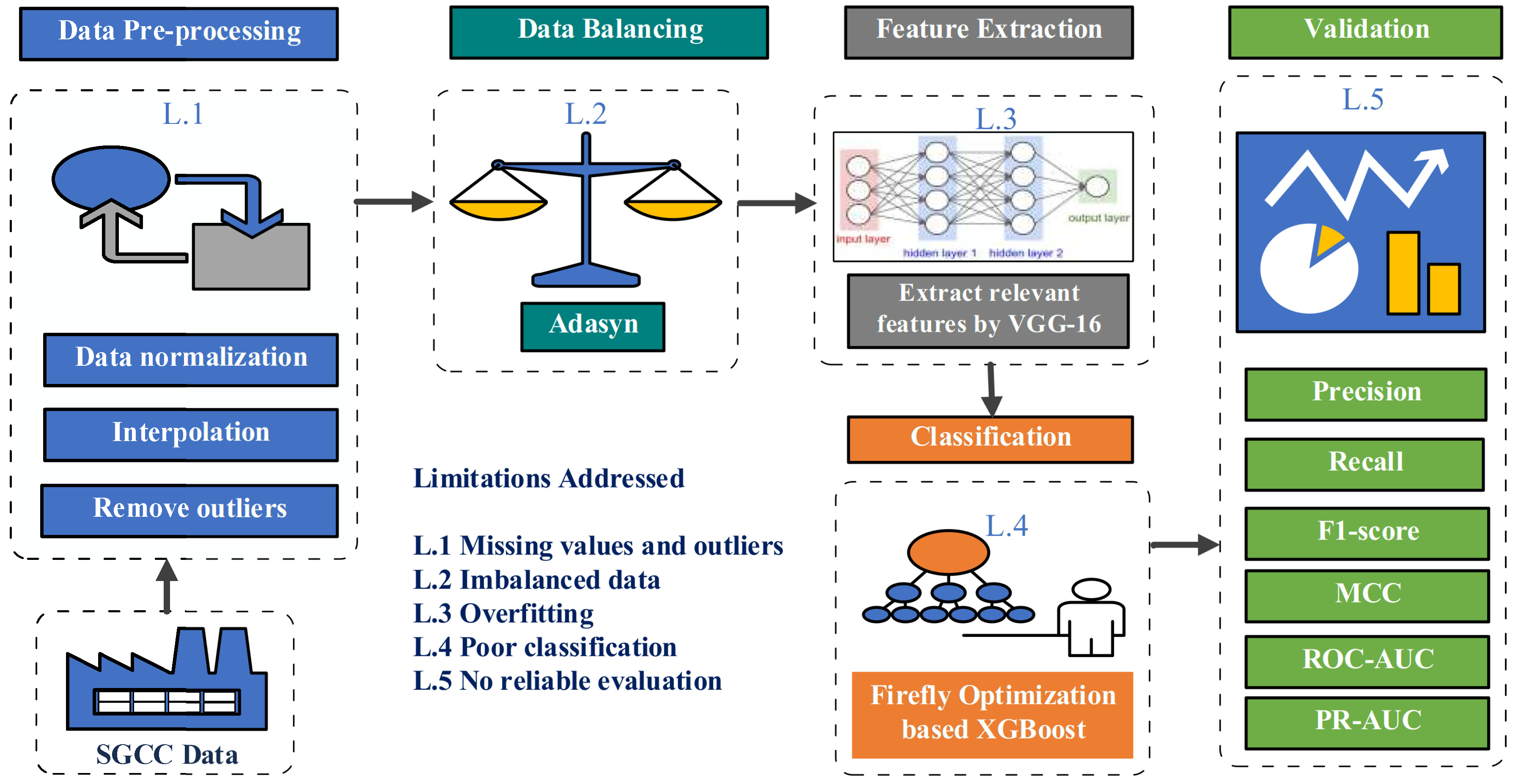
- A comprehensive data pre-processing is performed using interpolation, three sigma rule, and normalization methods to deal with missing values and outliers in the dataset. The data pre-processing step gives the refined input, which improves the performance of the classifier.
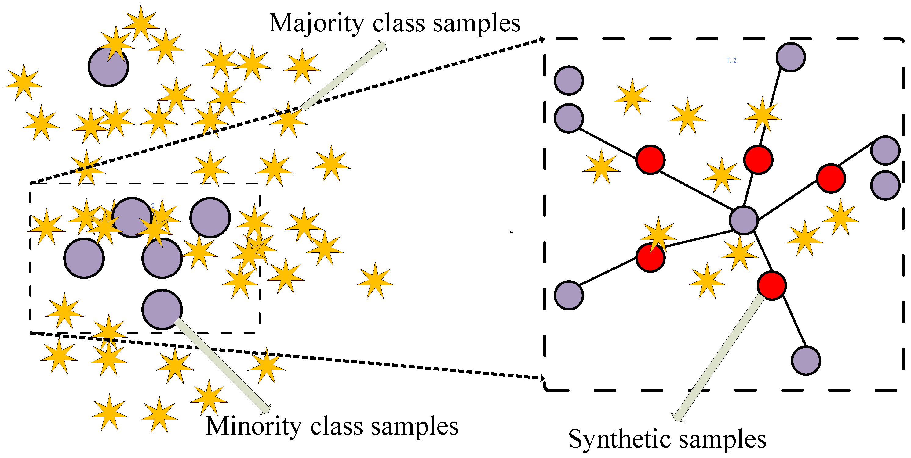
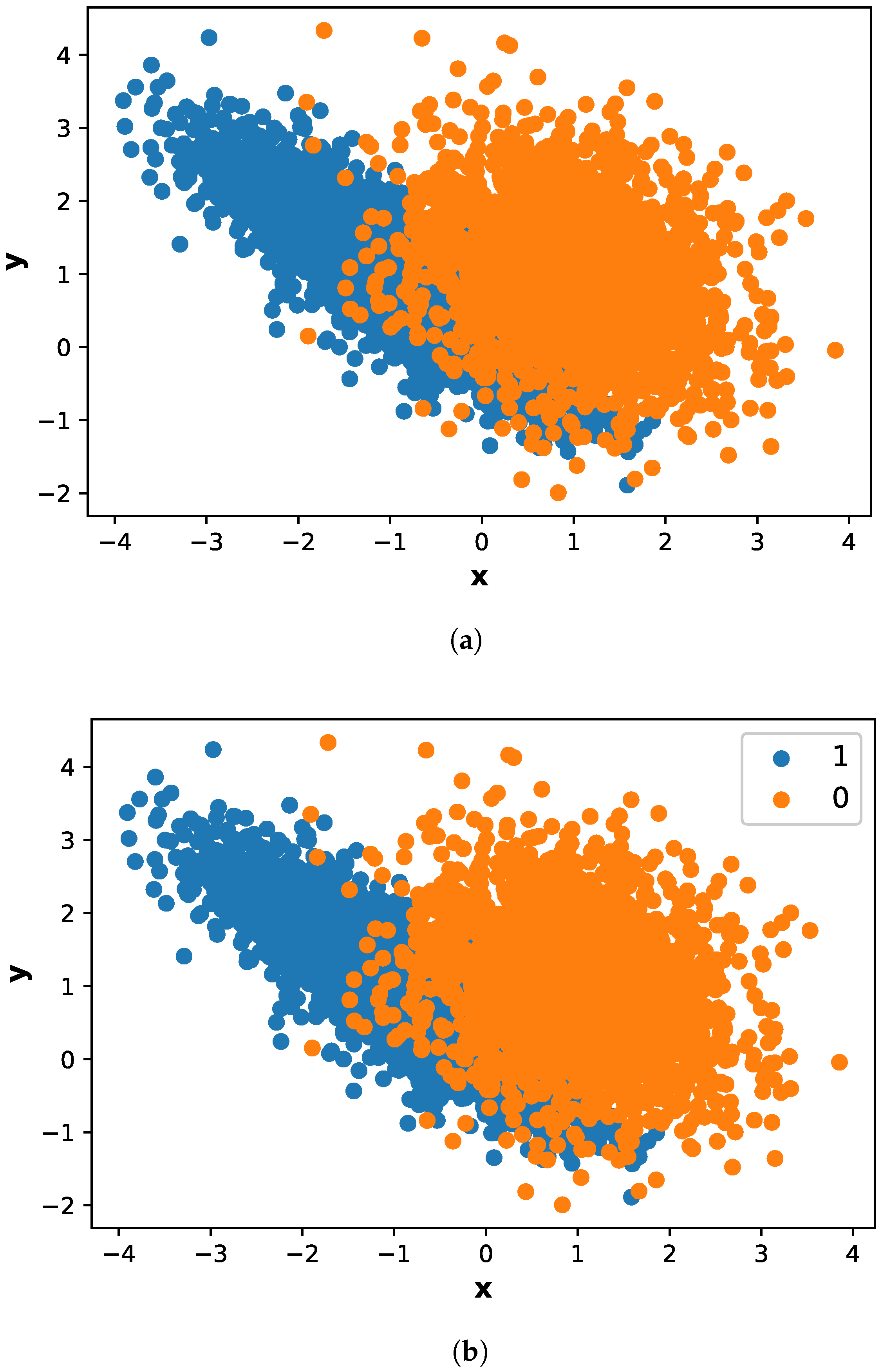
- A class balancing technique, Adasyn, is proposed to address the problem of imbalance data. The benefit of using Adasyn is two-fold. Firstly, it improves the learning performance of classifier to be more focused on theft cases that are harder to learn. Secondly, it prevents the model from being biased.
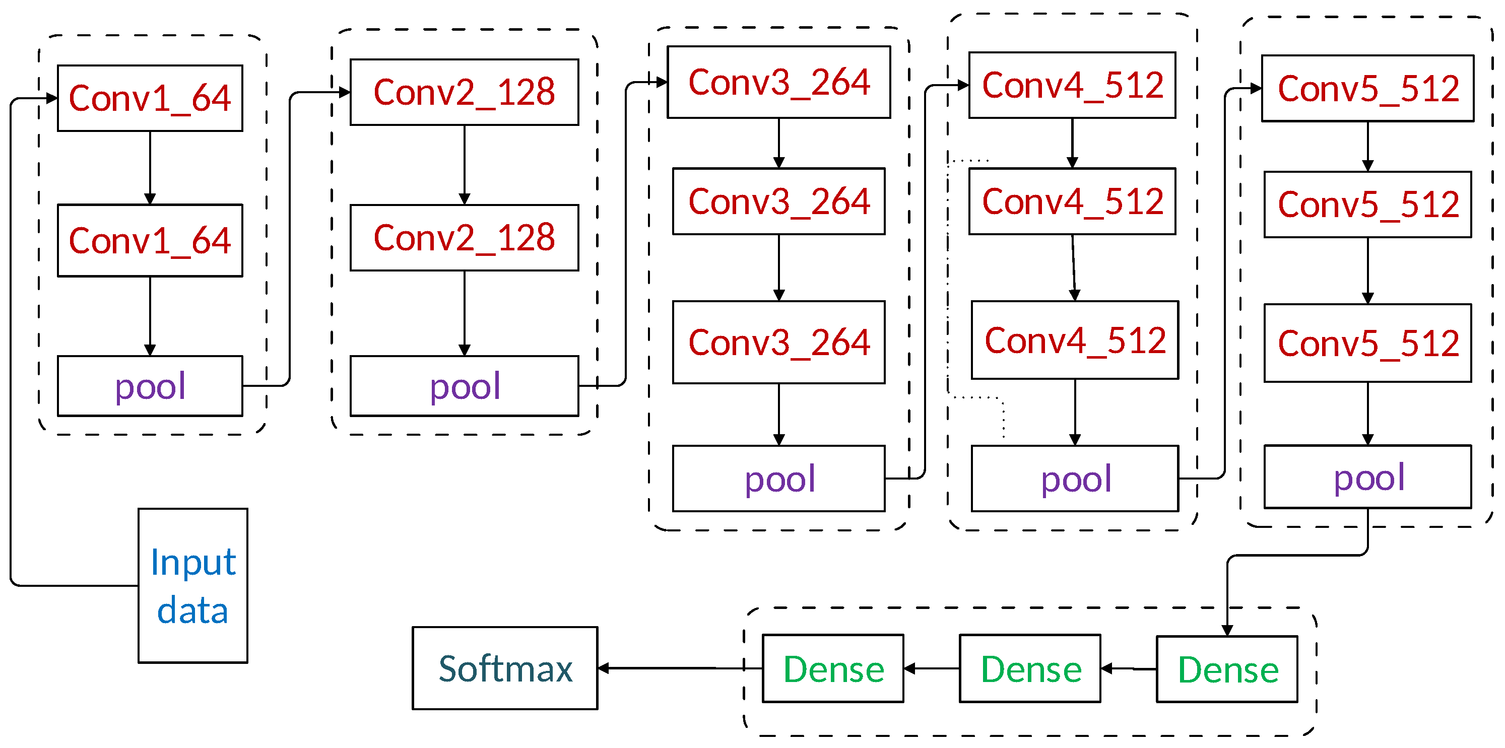
- We have introduced a new technique VGG-16 to solve the problem of overfitting to improve the classification performance. This technique is never being used before in ETD domain, and it has improved the accuracy of the classification model. The VGG-16 efficiently extracts useful information from data to truly represent electricity theft cases.
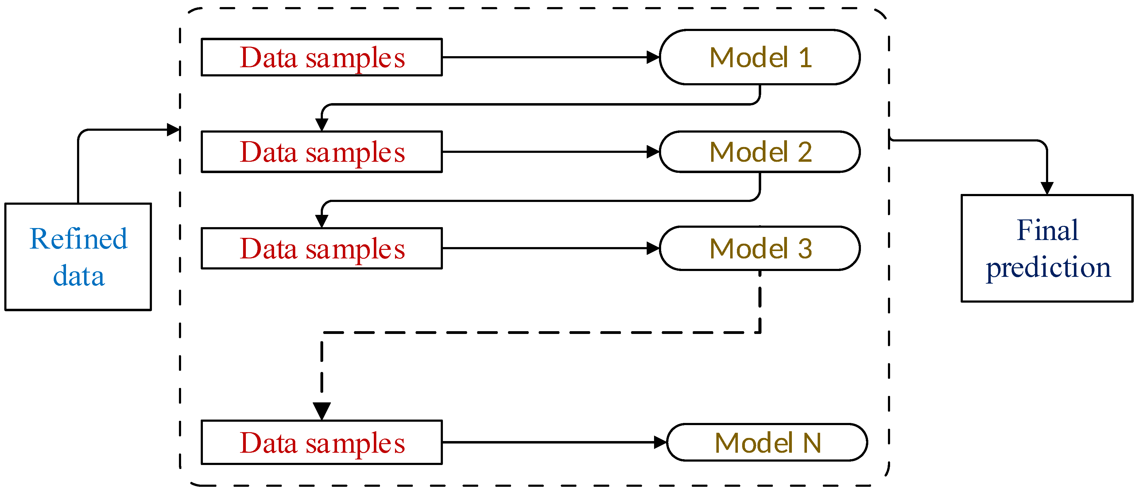
- XGBoost is applied to predict final classification, which improves the performance by combining multiple weak learners to make a strong learner.
- Along with XGBoost, an optimization technique, the Firefly Algorithm (FA) is utilized for efficient parameter optimization of the classifier.
- We conduct extensive simulations on real electricity consumption data set and for comparative analysis, precision, recall, F1-score, Matthews Correlation Coefficient (MCC), Receiving Operating Characteristics Area Under Curve (ROC-AUC), and Precision Recall Area Under Curve (PR-AUC) are used as performance metrics.
1.4. Organization of Paper
2. Proposed System Model
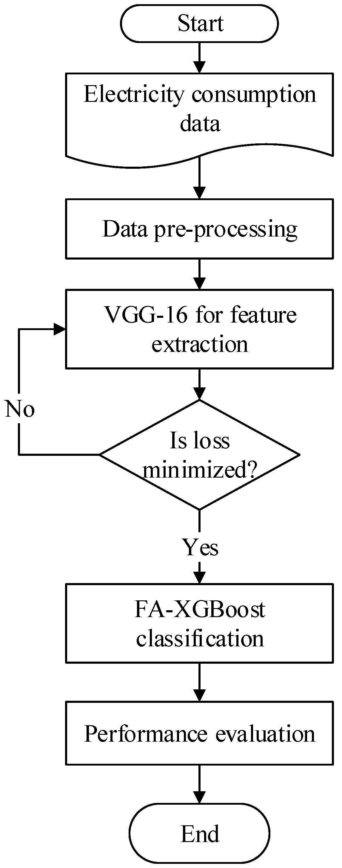
2.1. Overview of Proposed Methodology
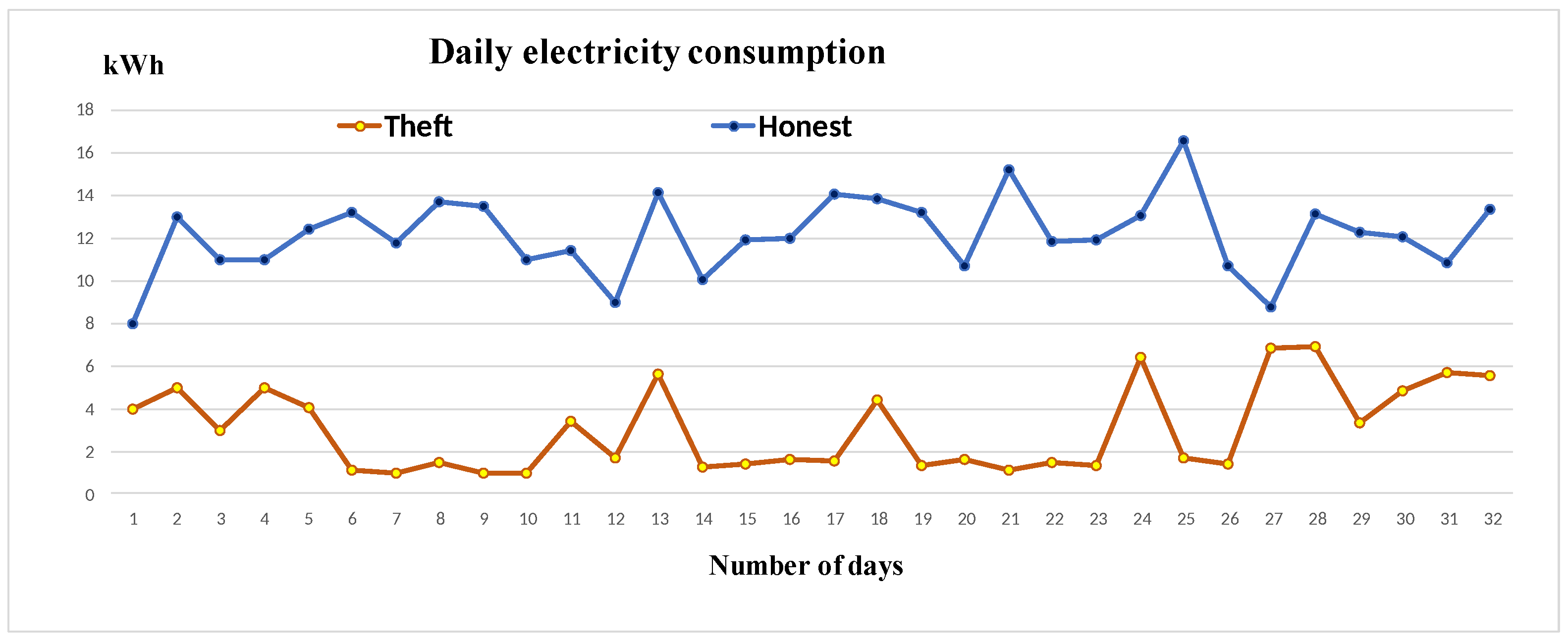
2.1.1. Information of Collected Data
2.1.2. Data Pre-Processing
2.1.3. Data Balancing
| Algorithm 1: Adasyn Algorithm |
| Input: Initial dataset X and desired balanced level Output: Synthetic dataset Initialize as minority class samples Initialize as majority class samples Synthesized total samples as for each do find the K nearest neighbors of end for for each do select the synthetic samples end for return |
2.1.4. Feature Extraction Using VGG-16
2.1.5. FA-XGBoost Based Classification
- Fireflies are uni-sexual in nature, so one firefly will be attracted to another regardless of whether the Firefly is male or female.
- The attractiveness is proportional to light intensity of each firefly; thus, for any two flashing fireflies, the less bright firefly will be attracted by the brightest firefly. Attractiveness is calculated using Equation (11), which is mentioned in [49] as:In the above equation, shows the attractiveness as a function of distance r, while represents attractiveness at zero distance. is the value of rate of light absorption in the air.
- As distance between fireflies increases, the attractiveness decreases. The distance between two fireflies i and j can be calculated using Euclidean distance as:where and are the components of the position of fireflies i and j, respectively, while d is the number of dimensions. If no firefly is found brighter in the initialized population, then it moves in a random direction. The random movement towards the most brighter firefly is calculated using Equation (13), which is mentioned in [49] as:In the above equation, rand represents the random number, t is the number of iterations, while controls the size of random walk.
| Algorithm 2: FA-XGBoost |
| 1: Set the objective function by y = (1,2,3 ... n) 2: Initialize the population of Fireflies by (i = 1,2,3 ... n) 3: Define as the rate of light absorption in the air 4: Define I as the light intensity of a firefly 5: Maximum number of iteration is m and t is current iteration 6: while (t < m) 7: for i = 1: 8: for j = 1: 9: if > then 10: Move Firefly i towards j 11: end if; 12: Attractiveness varies with distance r as given in Equation (8) 13: Adjust the light intensity I to find new solutions 14: Choose the best solution by random fly 15: end for j 16: end for i 17: Rank the Fireflies on the basis of minimum cost function 18: Choose the current best solution 19: end while 20: Return the best values of performance metrics |
3. Experiments and Results
3.1. Loss Function
3.2. Model Evaluation Metrics
- True positive (TP), the dishonest consumers accurately predicted as dishonest.
- True Negative (TN), the honest consumers accurately predicted as honest.
- False Positive (FP), the honest consumers predicted as thieves.
- False Negative (FN), the dishonest consumers predicted as honest consumers.
3.3. Benchmark Models and Their Configuration
3.3.1. SVM Model
3.3.2. LR Model
3.3.3. RUSBoost Model
3.3.4. CNN Model
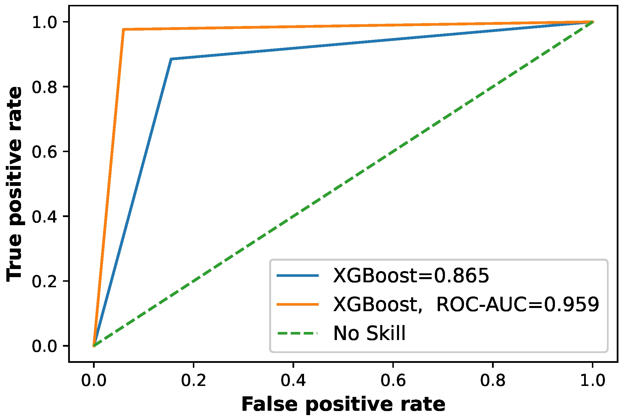
3.4. Proposed Model Results
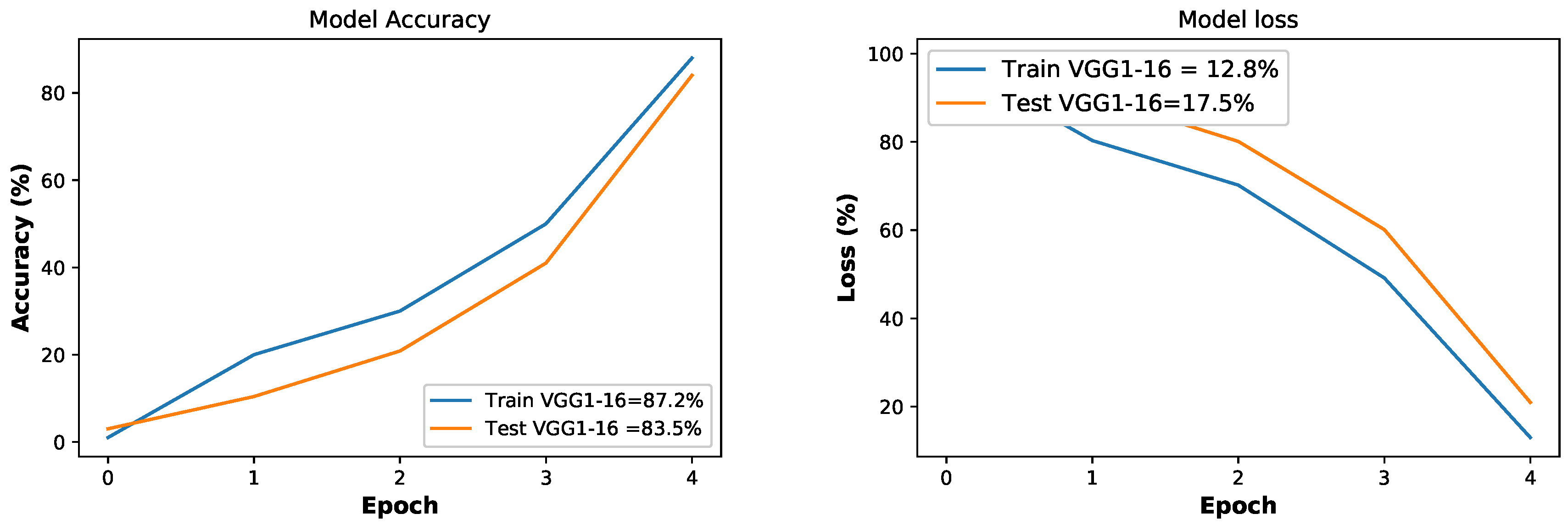
3.5. Convergence Analysis
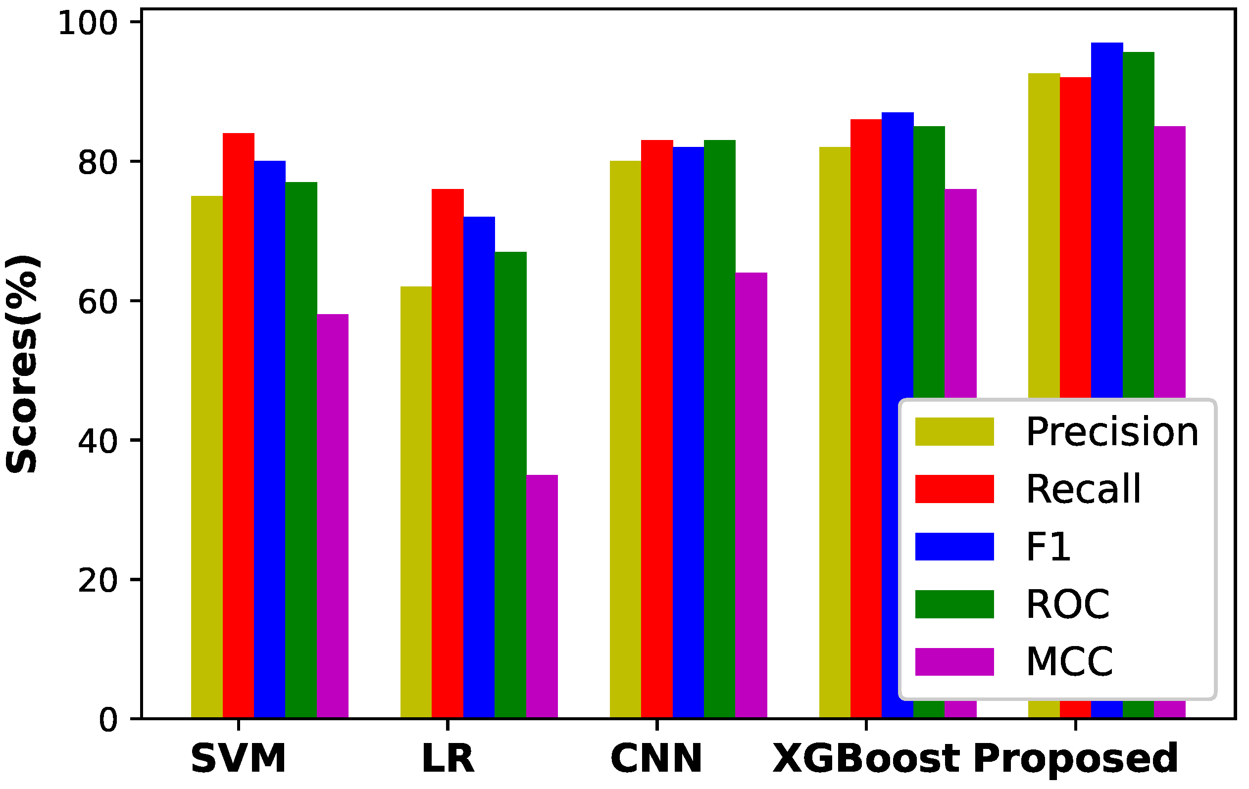
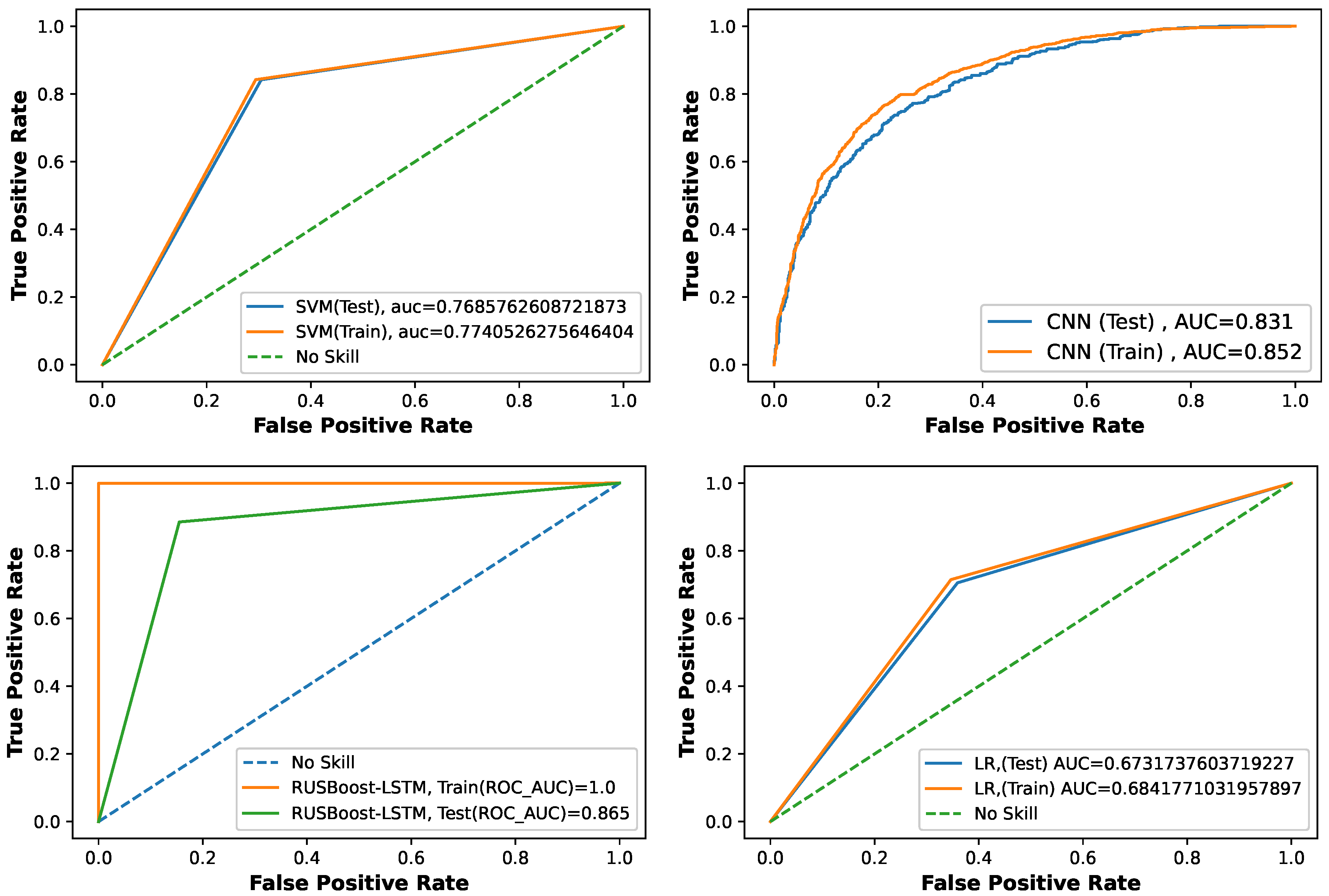
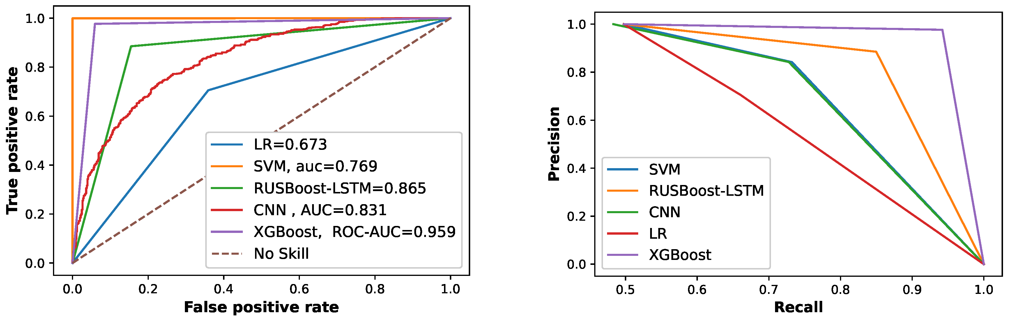
3.6. Comparison with Benchmark Models

4. Conclusions and Future Work
Author Contributions
Funding
Conflicts of Interest
References
- Gul, H.; Javaid, N.; Ullah, I.; Qamar, A.M.; Afzal, M.K.; Joshi, G.P. Detection of Non-Technical Losses using SOSTLink and Bidirectional Gated Recurrent Unit to Secure Smart Meters. Appl. Sci. 2020, 10, 3151. [Google Scholar] [CrossRef]
- Adil, M.; Javaid, N.; Qasim, U.; Ullah, I.; Shafiq, M.; Choi, J.-G. LSTM and Bat-Based RUSBoost Approach for Electricity Theft Detection. Appl. Sci. 2020, 10, 1–21. [Google Scholar]
- Mujeeb, S.; Javaid, N. ESAENARX and DE-RELM: Novel schemes for big data predictive analytics of electricity load and price. Sustain. Cities Soc. 2019, 51, 101642. [Google Scholar] [CrossRef]
- Nazari-Heris, M.; Mirzaei, M.A.; Mohammadi-Ivatloo, B.; Marzb, M.; Asadi, S. Economic-environmental effect of power to gas technology in coupled electricity and gas systems with price-responsive shiftable loads. J. Clean. Prod. 2020, 244, 118769. [Google Scholar] [CrossRef]
- Marzb, M.; Azarinejadian, F.; Savaghebi, M.; Pouresmaeil, E.; Guerrero, J.M.; Lightbody, G. Smart transactive energy framework in grid-connected multiple home microgrids under independent and coalition operations. Renew. Energy 2018, 126, 95–106. [Google Scholar]
- Jadidbonab, M.; Mohammadi-Ivatloo, B.; Marzb, M.; Siano, P. Short-term Self-Scheduling of Virtual Energy Hub Plant within Thermal Energy Market. IEEE Trans. Ind. Electron. 2020. accepted. [Google Scholar] [CrossRef] [Green Version]
- Gholinejad, H.R.; Loni, A.; Adabi, J.; Marzb, M. A hierarchical energy management system for multiple home energy hubs in neighborhood grids. J. Build. Eng. 2020, 28, 101028. [Google Scholar] [CrossRef]
- Mirzaei, M.A.; Sadeghi-Yazdankhah, A.; Mohammadi-Ivatloo, B.; Marzb, M.; Shafie-khah, M.; Catalão, J.P. Integration of emerging resources in IGDT-based robust scheduling of combined power and natural gas systems considering flexible ramping products. Energy 2019, 189, 116195. [Google Scholar] [CrossRef]
- Biswas, P.P.; Cai, H.; Zhou, B.; Chen, B.; Mashima, D.; Zheng, V.W. Electricity Theft Pinpointing through Correlation Analysis of Master and Individual Meter Readings. IEEE Trans. Smart Grid 2019, 11, 3031–3042. [Google Scholar] [CrossRef]
- Lydia, M.; Kumar, G.E.P.; Levron, Y. Detection of Electricity Theft based on Compressed Sensing. In Proceedings of the 2019 5th International Conference on Advanced Computing and Communication Systems (ICACCS) IEEE, Coimbatore, India, 15–16 March 2019; pp. 995–1000. [Google Scholar]
- Razavi, R.; Gharipour, A.; Fleury, M.; Akpan, I.J. A practical feature-engineering framework for electricity theft detection in smart grids. Appl. Energy 2019, 238, 481–494. [Google Scholar] [CrossRef]
- Depuru, S.S.S.R.; Wang, L.; Devabhaktuni, V. Support vector machine based data classification for detection of electricity theft. In Proceedings of the 2011 IEEE/PES Power Systems Conference and Exposition, Phoenix, AZ, USA, 20–23 March 2011; pp. 1–8. [Google Scholar]
- Saeed, M.S.; Mustafa, M.W.; Sheikh, U.U.; Jumani, T.A.; Mirjat, N.H. Ensemble Bagged Tree Based Classification for Reducing Non-Technical Losses in Multan Electric Power Company of Pakistan. Electronics 2019, 8, 860. [Google Scholar] [CrossRef] [Green Version]
- Razavi, R.; Fleury, M. Socio-economic predictors of electricity theft in developing countries: An Indian case study. Energy Sustain. Dev. 2019, 49, 1–10. [Google Scholar] [CrossRef]
- McDaniel, P.; McLaughlin, S. Security and privacy challenges in the smart grid. IEEE Secur. Priv. 2009, 7, 75–77. [Google Scholar] [CrossRef]
- Buzau, M.M.; Tejedor-Aguilera, J.; Cruz-Romero, P.; Gomez-Exposito, A. Hybrid deep neural networks for detection of non-technical losses in electricity smart meters. IEEE Trans. Power Syst. 2019, 35, 1254–1263. [Google Scholar] [CrossRef]
- Jamil, A.; Alghamdi, T.A.; Khan, Z.A.; Javaid, S.; Haseeb, A.; Wadud, Z.; Javaid, N. An Innovative Home Energy Management Model with Coordination among Appliances using Game Theory. Sustainability 2019, 11, 6287. [Google Scholar] [CrossRef]
- Buzau, M.M.; Tejedor-Aguilera, J.; Cruz-Romero, P.; Gómez-Expósito, A. Detection of non-technical losses using smart meter data and supervised learning. IEEE Trans. Smart Grid 2018, 10, 2661–2670. [Google Scholar] [CrossRef]
- Hasan, M.; Toma, R.N.; Nahid, A.A.; Islam, M.M.; Kim, J.M. Electricity Theft Detection in Smart Grid Systems: A CNN-LSTM Based Approach. Energies 2019, 12, 3310. [Google Scholar] [CrossRef] [Green Version]
- Avila, N.F.; Figueroa, G.; Chu, C.C. NTL detection in electric distribution systems using the maximal overlap discrete wavelet-packet transform and random under sampling boosting. IEEE Trans. Power Syst. 2018, 33, 7171–7180. [Google Scholar]
- Ramos, C.C.; Rodrigues, D.; de Souza, A.N.; Papa, J.P. On the study of commercial losses in Brazil: A binary black hole algorithm for theft characterization. IEEE Trans. Smart Grid 2016, 9, 676–683. [Google Scholar] [CrossRef]
- Zheng, K.; Chen, Q.; Wang, Y.; Kang, C.; Xia, Q. A novel combined data-driven approach for electricity theft detection. IEEE Trans. Ind. Inform. 2019, 15, 1809–1819. [Google Scholar] [CrossRef]
- Ding, N.; Ma, H.; Gao, H.; Ma, Y.; Tan, G. Real-time anomaly detection based on long short-Term memory and Gaussian Mixture Model. Comput. Electr. Eng. 2019, 70, 106458. [Google Scholar] [CrossRef]
- Li, S.; Han, Y.; Yao, X.; Yingchen, S.; Wang, J.; Zhao, Q. Electricity Theft Detection in Power Grids with Deep Learning and Random Forests. J. Electr. Comput. Eng. 2019, 2019, 1–12. [Google Scholar] [CrossRef]
- Punmiya, R.; Choe, S. Energy theft detection using gradient boosting theft detector with feature engineering-based preprocessing. IEEE Trans. Smart Grid 2019, 10, 2326–2329. [Google Scholar] [CrossRef]
- Amin, S.; Schwartz, G.A.; Cardenas, A.A.; Sastry, S.S. Gametheoretic models of electricity theft detection in smart utility networks: Providing new capabilities with advanced metering infrastructure. IEEE Control. Syst. Mag. 2015, 35, 66–81. [Google Scholar]
- Leite, J.B.; Mantovani, J.R.S. Detecting and locating non-technical losses in modern distribution networks. IEEE Trans. Smart Grid 2016, 9, 1023–1032. [Google Scholar] [CrossRef] [Green Version]
- Wang, S.; Chen, H. A novel deep learning method for the classification of power quality disturbances using deep convolutional neural network. Appl. Energy 2019, 235, 1126–1140. [Google Scholar] [CrossRef]
- State Grid Corporation of China. Available online: https://www.sgcc.com.cn (accessed on 22 February 2020).
- Zheng, Z.; Yang, Y.; Niu, X.; Dai, H.N.; Zhou, Y. Wide and deep convolutional neural networks for electricity-theft detection to secure smart grids. IEEE Trans. Ind. Informat. 2017, 14, 1606–1615. [Google Scholar] [CrossRef]
- Chola, V.; Banerjee, A.; Kumar, V. Anomaly detection: A survey. Acm Comput. Surv. (Csur) 2009, 41, 1–58. [Google Scholar]
- Nam, H.; Kim, H.E. Batch-instance normalization for adaptively style-invariant neural networks. In Advances in Neural Information Processing Systems; The MIT Press: Cambridge, MA, USA, 2018; pp. 2558–2567. [Google Scholar]
- Pandey, A.; Jain, A. Comparative analysis of KNN algorithm using various normalization techniques. Int. J. Comput. Netw. Inf. Secur. 2017, 9, 36–42. [Google Scholar] [CrossRef] [Green Version]
- Figueroa, G.; Chen, Y.S.; Avila, N.; Chu, C.C. Improved practices in machine learning algorithm for NTL detection with imbalanced data. In Proceedings of the 2017 IEEE Power Energy Society General Meeting, Chicago, IL, USA, 16–20 July 2017; pp. 1–5. [Google Scholar]
- Hasanin, T.; Khoshgoftaar, T. The effects of random under sampling with simulated class imbalance for big data. In Proceedings of the 2018 IEEE International Conference on Information Reuse and Integration (IRI), Salt Lake City, UT, USA, 6–9 July 2018; pp. 70–79. [Google Scholar]
- Qin, H.; Zhou, H.; Cao, J. Imbalanced Learning Algorithm based Intelligent Abnormal Electricity Consumption Detection. Neurocomputing 2020, 402, 112–123. [Google Scholar]
- Qu, Z.; Li, H.; Wang, Y.; Zhang, J.; Abu-Siada, A.; Yao, Y. Detection of Electricity Theft Behavior Based on Improved Synthetic Minority Oversampling Technique and Random Forest Classifier. Energies 2020, 13, 2039. [Google Scholar] [CrossRef]
- Pelayo, L.; Dick, S. Synthetic minority oversampling for function approximation problems. Int. J. Intell. Syst. 2019, 34, 2741–2768. [Google Scholar] [CrossRef]
- He, H.; Bai, Y.; Garcia, E.A.; Li, S. ADASYN: Adaptive synthetic sampling approach for imbalanced learning. In Proceedings of the 2008 IEEE International Joint Conference on Neural Networks (IEEE world Congress on Computational Intelligence), Hong Kong, China, 1–8 June 2008. [Google Scholar]
- Xiang, Y. Polarity Classification of Imbalanced Microblog Texts; AIST: Tsukuba, Ibaraki, Japan, 2019; pp. 1–61. [Google Scholar]
- Simonyan, K.; Zisserman, A. Very Deep Convolutional Networks for Large-Scale Image Recognition. arXiv 2014, arXiv:1409.1556. [Google Scholar]
- Yu, W.; Yang, K.; Bai, Y.; Xiao, T.; Yao, H.; Rui, Y. Visualizing and comparing AlexNet and VGG using deconvolutional layers. In Proceedings of the 33rd International Conference on Machine Learning, New York City, NY, USA, 19–24 June 2016; pp. 1–7. [Google Scholar]
- Dixon, J.; Rahman, M. Modality Detection and Classification of Biomedical Images with Deep Transfer Learning and Feature Extraction. In Proceedings of the International Conference on Image Processing, Computer Vision, and Pattern Recognition (IPCV) The Steering Committee of The World Congress in Computer Science, Computer Engineering and Applied Computing (WorldComp), Las Vegas, NV, USA, 29 July–1 August 2019; pp. 55–58. [Google Scholar]
- Cıbuk, M.; Budak, U.; Guo, Y.; Ince, M.C.; Sengur, A. Efficient deep features selections and classification for flower species recognition. Measurement 2019, 137, 7–13. [Google Scholar] [CrossRef]
- Chen, T.; Guestrin, C. XGBoost: A scalable tree boosting system. In Proceedings of the 22nd ACM SIGKDD Conference on Knowledge Discovery and Data Mining, San Francisco, CA, USA, 13–17 August 2016; pp. 785–794. [Google Scholar]
- Zahid, M.; Ahmed, F.; Javaid, N.; Abid Abbasi, R.; Zainab Kazmi, H.S.; Javaid, A.; Bilal, M.; Akbar, M.; Ilahi, M. Electricity Price and Load Forecasting using Enhanced Convolutional Neural Network and Enhanced Support Vector Regression in Smart Grids. Electronics 2019, 8, 122. [Google Scholar] [CrossRef] [Green Version]
- Yang, X.-S. Firefly Algorithm, Stochastic Test Functions and Design Optimization. Int. Bio-Inspired Comput. 2010, 2, 78–84. [Google Scholar] [CrossRef]
- Yang, X.S. Chaos-enhanced firefly algorithm with automatic parameter tuning. In Recent Algorithms and Applications in Swarm Intelligence Research; Information Science Reference (IGI Global): Hershey, PA, USA, 2013; pp. 125–136. [Google Scholar]
- Chen, K.; Zhou, Y.; Zhang, Z.; Dai, M.; Chao, Y.; Shi, J. Multilevel image segmentation based on an improved firefly algorithm. Math. Probl. Eng. 2016, 2016, 1–12. [Google Scholar] [CrossRef]
- Janocha, K.; Czarnecki, W.M. On loss functions for deep neural networks in classification. arXiv 2017, arXiv:1702.05659. [Google Scholar] [CrossRef]
- Zhu, W.; Zeng, N.; Wang, N. Sensitivity, specificity, accuracy, associated confidence interval and ROC analysis with practical SAS implementations. Nesug Proc. Health Care Life Sci. Balt. Md. 2010, 19, 67. [Google Scholar]


| Methods | Contributions | Limitations |
|---|---|---|
| Hardware based [16] | Its focus is on designing specific hardware devices in order to detect electricity theft | High cost of hardware installation |
| Game theory [17] | There is a game between the electricity thieves and the utility. The outcome of a game can be derived from the difference between the electricity consumption behavior of electricity thieves and benign users | This method needs to define a utility function for all the players in a game, which is quite challenging. |
| Machine learning [18,19,20,21,22,23,24,25] | It uses the smart meter data to effectively detect anomalous consumption behavior of dishonest consumers | Performance is poor on highly imbalanced data |
| Dataset | Supervised Techniques | Data Balancing | Contributions | Limitations |
|---|---|---|---|---|
| SGCC [19] | LSTM, CNN | SMOTE | The CNN is utilized for feature extraction, while LSTM uses the refined features to classify the data into honest consumers and electricity thieves. | The overfitting problem is not considered, which is caused by the addition of duplicate information through SMOTE |
| Endesa [16] | MLP and LSTM | Not handled | Detect the NTL by combining the auxiliary data through MLP and electricity consumption data through LSTM | The imbalanced data are not balanced before classification |
| Honduras [20] | MODWPT, RUSBoost | National grid of Brazil | The MODWPT gives the refined input and RUSBoost method balances the labels in the data before classification | The random under sampling technique reduces the data size and results in underfitting the model |
| Brazilian utility [21] | BBHA | Not handled | Use of binary black hole optimization technique to identify the NTL | No reliable evaluation is performed to validate the performance of the system |
| Endesa [18] | SVM, XGBoost | RUS | The XGBoost is utilized that operates as an ensemble method and boosts the classification performance | The data pre-processing is not considered to refine the input data |
| Irish data [22] | MIC, FSFD | Not handled | The refined data are achieved by MIC method, while FSFDP is used for classification. | This model has a high cost of hardware installation |
| NAB [23] | LSTM-GMM | Not handled | The authors enhanced the internal structure of LSTM to solve the gradient vanishing problem | The model is complex and its execution time is high |
| EISA [24] | CNN, RF | SMOTE | The generalized performance is achieved by using the decision trees along with CNN | The SMOTE generate synthetic data, which causes overfitting issues |
| Limitation Number | Limitation Identified | Solution Number | Proposed Solution |
|---|---|---|---|
| L.1 | Missing values and outliers | S.1 | Pre-processing |
| L.2 | Imbalanced data | S.2 | Adasyn |
| L.3 | Overfitting | S.3 | VGG-16 |
| L.4 | Weak classification | S.4 | FA-XGBoost |
| L.5 | Reliable Evaluation | S.5 | Precision, Recall, F1-Score, |
| MCC, ROC-AUC, PR-AUC |
| Description | Values |
|---|---|
| Duration of collected data | 2014–2016 |
| Data type | Time series |
| Dimension | 1034 |
| Samples | 42,372 |
| Resolution | High resolution real time smart meter data |
| Number of fraudulent consumers | 3800 |
| Number of honest consumers | 38,530 |
| Total consumers | 42,372 |
| Hyper-Parameters | Values | Description |
|---|---|---|
| Batch size | 130 | It is training samples in each iteration |
| Leaning rate | 0.001 | It is a tuning parameter |
| Dropout | 0.01 | To avoid overfitting problem in neural networks. |
| Optimizer | Adam | It is adaptive learning rate. |
| Epochs | 10 | It is the number of iterations for training the algorithm |
| Hyper-Parameters | Range of Values | Selected Value |
|---|---|---|
| 1, 3, 5 | 3 | |
| C | 0.001, 0.01, | 0.01 |
| Hyper-Parameters | Range of Values | Selected Value |
|---|---|---|
| R | 0.001, 0.01, 0.1 | 0.001 |
| C | l1 norm, l2 norm | l2 norm |
| Hyper-Parameters | Range of Values | Selected Value |
|---|---|---|
| Learning rate | 0.2, 0.5, 1 | 1 |
| Estimator | 150, 200, 300 | 200 |
| Hyper-Parameters | Range of Values | Selected Value |
|---|---|---|
| Epochs | 10, 15, 30 | 10 |
| Batch size | 50, 80, 130 | 50 |
| Dropout | 0.01, 0.1, 0.2 | 0.2 |
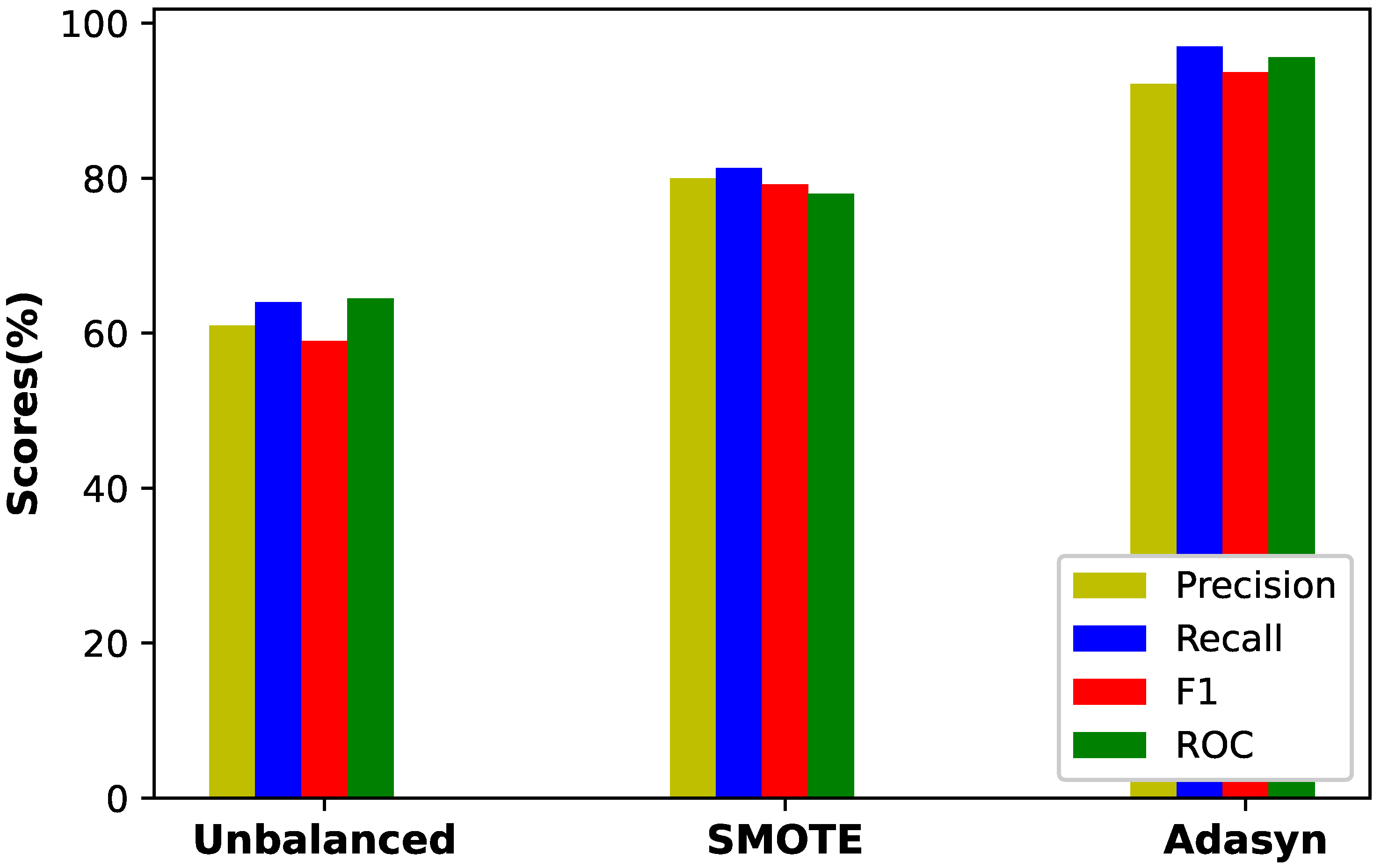
| Performance Metrics | Imbalaced Data | SMOTE | Adasyn |
|---|---|---|---|
| Precision | 60 | 79.1 | 93 |
| Recall | 62.1 | 80 | 97 |
| F1-score | 59.01 | 78.7 | 93.7 |
| ROC-AUC | 63.2 | 78 | 95.9 |
| Confusion Matrix | Predicted No | Predicted Yes |
|---|---|---|
| Actual No | TN = 9306 | FP = 1296 |
| Actual Yes | FN = 948 | TP= 8996 |
| Limitation Number | Limitation Identified | Solution Number | Validation Results |
|---|---|---|---|
| L.1 | Missing values and outliers | S.1 | No direct validation |
| L.2 | Imbalanced data | S.2 | Adasyn algorithm effectively |
| handles imbalance data as | |||
| shown in Figure 8 | |||
| L.3 | Overfitting | S.3 | Figure 10 shows a |
| generalized performance of our | |||
| proposed model | |||
| L.4 | Poor classification | S.4 | Firefly based XGBoost classifier |
| achieved excellent results in | |||
| terms of all performance metrics | |||
| as mentioned in Figure 9 | |||
| L.5 | No reliable Evaluation | S.5 | Figure 11 shows the performance |
| of our proposed model in terms | |||
| of several performance metrics |
| Models | Accuracy | Precision | Recall | F1-Score | ROC | MCC |
|---|---|---|---|---|---|---|
| CNN | 0.812 | 0.805 | 0.862 | 0.845 | 0.813 | 61.5 |
| SVM | 0.772 | 0.765 | 0.883 | 0.819 | 0.769 | 56.3 |
| LR | 0.676 | 0.645 | 0.772 | 0.701 | 0.673 | 35.6 |
| RUSBoost | 0.869 | 0.85 | 0.896 | 0.871 | 0.865 | 77.8 |
| Proposed Model | 0.95 | 0.930 | 0.9700 | 0.937 | 0.959 | 85.6 |
© 2020 by the authors. Licensee MDPI, Basel, Switzerland. This article is an open access article distributed under the terms and conditions of the Creative Commons Attribution (CC BY) license (http://creativecommons.org/licenses/by/4.0/).
Share and Cite
Khan, Z.A.; Adil, M.; Javaid, N.; Saqib, M.N.; Shafiq, M.; Choi, J.-G. Electricity Theft Detection Using Supervised Learning Techniques on Smart Meter Data. Sustainability 2020, 12, 8023. https://doi.org/10.3390/su12198023
Khan ZA, Adil M, Javaid N, Saqib MN, Shafiq M, Choi J-G. Electricity Theft Detection Using Supervised Learning Techniques on Smart Meter Data. Sustainability. 2020; 12(19):8023. https://doi.org/10.3390/su12198023
Chicago/Turabian StyleKhan, Zahoor Ali, Muhammad Adil, Nadeem Javaid, Malik Najmus Saqib, Muhammad Shafiq, and Jin-Ghoo Choi. 2020. "Electricity Theft Detection Using Supervised Learning Techniques on Smart Meter Data" Sustainability 12, no. 19: 8023. https://doi.org/10.3390/su12198023