A Novel Command-Filtered Adaptive Backstepping Control Strategy with Prescribed Performance for Photovoltaic Grid-Connected Systems

Abstract

With the aim of solving the power fluctuation and bus voltage instability problems caused by external environment variations in the photovoltaic grid-connected system, a prescribed performance-based adaptive backstepping controller is proposed for the system to regulate the bus voltage and the inverter current. First, the mathematical model of the grid-connected inverter is established, in which the uncertain system parameters are estimated via a designed projection-based adaptive law. Then, the command-filtered backstepping sliding mode control method is applied to the system for power regulation. In order to achieve favorable tracking performance, the prescribed performance technique is introduced in the voltage regulation strategy by constraining the compensated voltage tracking error within a certain range from a novel point of view. Finally, the simulation is carried out considering the variations of environmental situations, and the obtained results demonstrate the sound performance of the prescribed performance-based control strategy with respect to the photovoltaic grid-connected system.

1. Introduction

With the depletion of fossil fuels and the call for environmental protection, more and more green power generation modes are being integrated into the power grid to supply power, among which the photovoltaic (PV) power generation is widely used with large-scale installed capacity for its high income, simple operation, and maintenance, as well as reasonable resource allocation [1,2,3]. However, the increasing share of these intermittent renewable electricity generations bring about great challenges to grid-balancing and power supply security [4,5,6]. Besides, considering the uncertain variations of the external environment containing the solar irradiation and temperature which results in the power fluctuation problem, it is essential to draft some measures to ensure the stability of the system [6].

There exist many investigations on the stabilization of the PV grid-connected system by researchers around the world [7,8,9,10,11]. From the point of view of the model of the PV grid-connected system, the Reference [7] studies the influence of nonlinearities like dead time and the phase-locked loop with regard to power quality and stability via the generalized Nyquist stability criterion, and verifies the theory with a simulation and experiment. In [8], a feedback linearization technique was introduced for the partial linearization of the three-phase PV grid-connected system, which promotes the design process of the controller, and the zero dynamic stability of the system was acquired under the designed controller, which helps transport the grid power. In terms of the control method with respect to the grid-connected system, a $H_{\infty }$ control method was brought to the grid-connected inverter in [9] to achieve the stable operation of the system when the grid impedance possibly varies, and the control performance proved better than conventional PID control. In [10], an adaptive sliding mode control method was used for the inverter of a single-phase PV grid-connected system for bus voltage stabilization, and the fuzzy neural network was employed for the estimation of system uncertainties. In [11], a command-filtered backstepping control (CBC) method was proposed to solve the voltage tracking and power fluctuation problems in the grid-connected system, and possessed better performance than PID. However, the concrete numerical control objectives are absent in [11] and the bus voltage is regulated indirectly by adjusting active power, which results in the lack of voltage tracking precision, and the simulation situations are set from the theoretical level without considering the actual conditions. Thus, the existed problems motivate us to continue research based on the backstepping control method to seek better performance.

The backstepping control method was first proposed by Farrell et al. in [12] to solve the tracking control problem in nonlinear systems, and the command filter was introduced to avoid the differential expansion problem. The corresponding controller design process was provided with certain procedures based on the Lyapunov stability criterion, which is much simpler than other advanced control approaches and attracts much attention. The theory of backstepping control has been studied widely, including several aspects like finite time, input saturation, and distributed control [13,14,15,16]. In terms of its applications, many advanced control strategies have been integrated with backstepping control to obtain better control performance and achieve a higher control objective in various fields, such as with the robot [17], ship [18], wind turbine [19], unmanned aerial vehicle [20,21]. On the other hand, the prescribed performance control (PPC) technique was introduced by Bechlioulis et al. in [22], which focuses on the tracking control accuracy and boundedness. The output tracking error is constrained within the prescribed range upon when the design process begins, and then converts to an equivalent error, which turns the restriction problem into an unrestricted one. On account of its boundedness with respect to the tracking error, the prescribed performance control gained extensive investigations [23,24,25,26,27]. According to the above investigation, the backstepping control integrated with prescribed performance control was selected for the PV grid-connected system for the voltage stabilization and power fluctuation reduction.

In general, the command-filtered adaptive backstepping sliding mode control approach was designed accompanied by the prescribed performance technique for the stable operation of the PV grid-connected system. The control objectives contain some aspects, namely, how the active power fluctuation shall be reduced, and the DC bus voltage shall be maintained stable around the reference with adequate tracking precision. Besides, the three-phase voltage of the inverter shall be kept stable and the harmonics reduced. The main contributions and innovations of this paper are listed in the following.

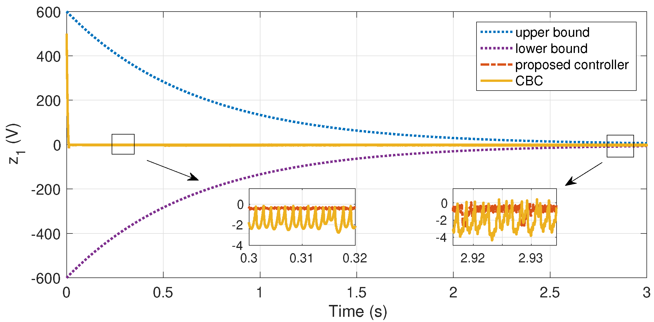
• The prescribed performance technique is introduced in the command-filtered backstepping sliding mode controller to constrain the voltage tracking error within the preset range, namely, enable the DC bus voltage which possesses the prescribed performance, which constitutes to the stable operation of the PV grid-connected system.
• The integral sliding mode control method is considered in the controller design process to improve the robustness of the system, and the stability of the prescribed performance-based control strategy is proved via the Lyapunov stability criterion.
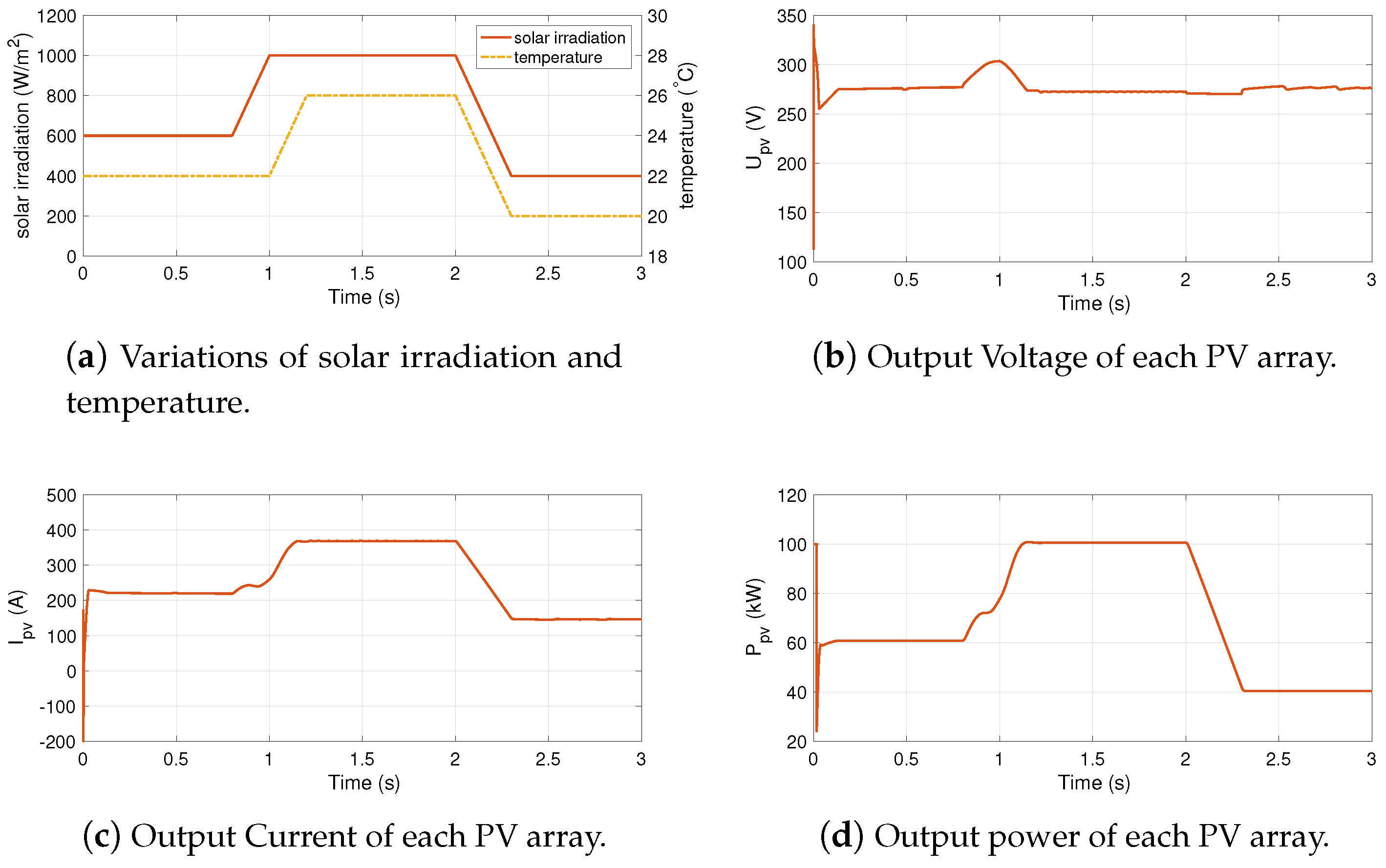
• The environmental variations of PV arrays, including solar irradiation and temperature, are reasonably considered in the system to test the stability of the control system.

The rest of the paper is organized as follows: Section 2 provides the preliminaries, including the mathematical modeling of the PV grid-connected system and basic knowledge of prescribed performance control. Based on the model, the controller is designed with the prescribed performance technique and the stability proof is offered. In Section 3, the simulation is carried out on the PV grid-connected system with the battery energy storage system (BESS), and the results are discussed to test the effectiveness of the proposed controller. Ultimately, some conclusions are drawn in Section 4.

2. Materials and Methods

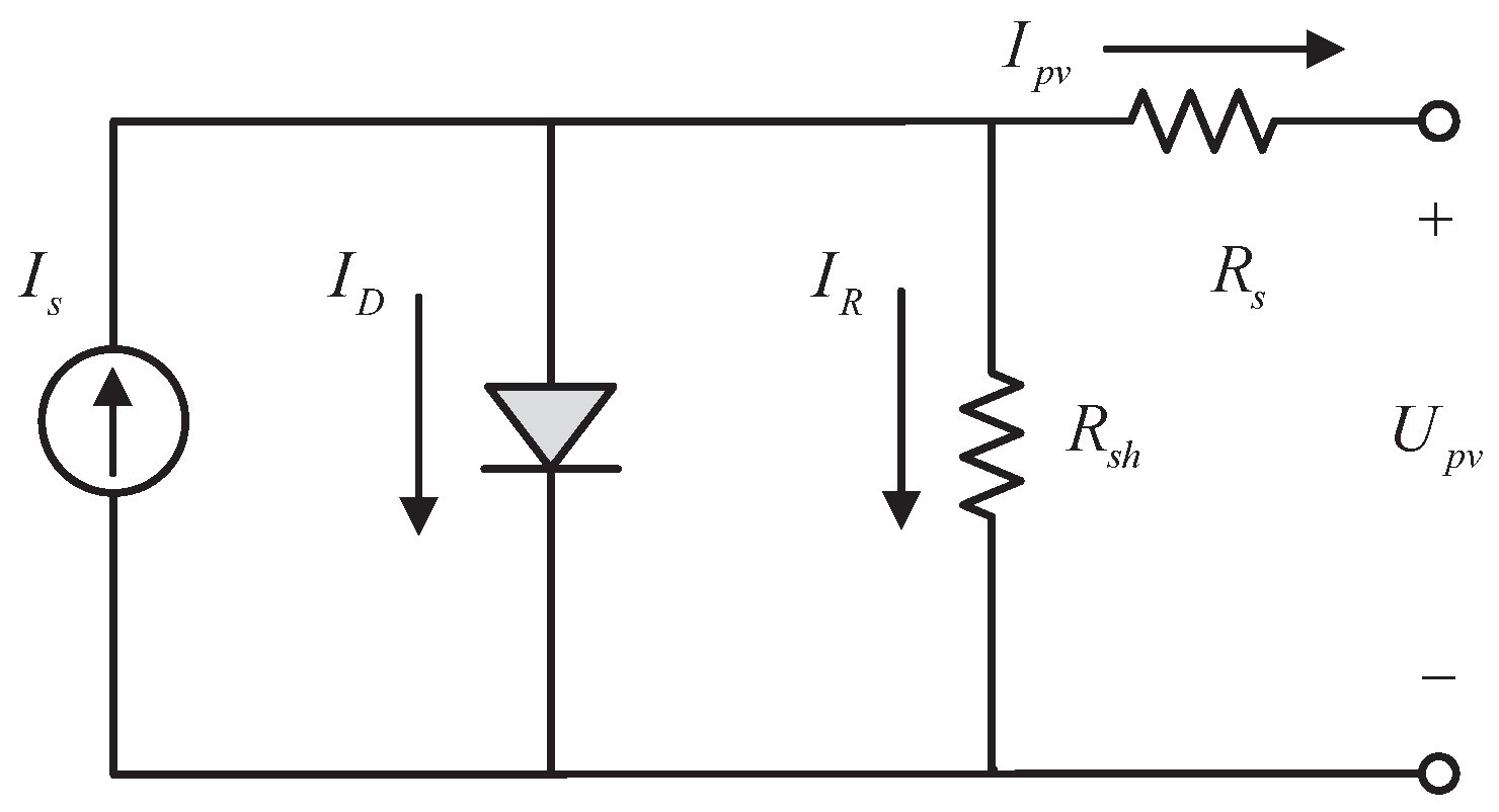
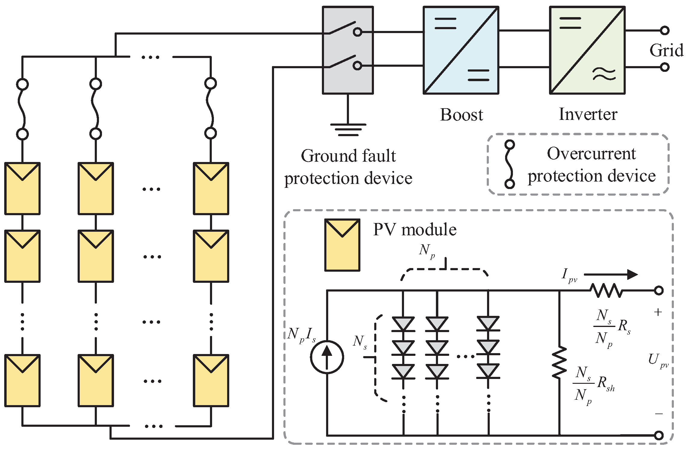
2.1. PV Arrays Modeling

The circuit topology of the PV cell is shown in Figure 1. The parameters in Figure 1 are explained as follows: $I_s$ is the photocurrent, $I_D$ the diode current, $R_{sh}$ is the shunt resistance, and $I_R$ is the corresponding current, $R_s$ is the series resistance, $I_{pv}$ is the output current of the cell, and $U_{pv}$ is the output voltage. First, the diode current $I_D$ can be expressed as [11,28]:

$$I_D=I_0\left(exp\left(\frac{q\left(U_{pv}+R_s{I}_{pv}\right)}{AkT}\right)-1\right),$$

(1)

where $I_0$ is the reverse saturation current, A is the dimensionless coefficient, q is the elementary charge ($q=1.6\times {10}^{-19}C$), k is the Boltzmann constant, and T is the temperature of the cell, which is counted in the Kelvin scale.

Referred to as Kirchhoff’s Current Law, the output current $I_{pv}$ generated by the PV cell in Figure 1 is represented as

$$I_{pv}=I_s-I_0\left(exp\left(\frac{q\left(U_{pv}+R_s{I}_{pv}\right)}{AkT{N}_s}\right)-1\right)-\frac{U_{pv}+R_s{I}_{pv}}{R_{sh}},$$

(2)

and its photocurrent $I_s$ can be represented as

$$I_s=\left(I_{sc}+k_i\left(T-T_n\right)\right)\frac{R_0}{R_n},$$

(3)

where $I_{sc}$ means the short-circuit current, $k_i$ denotes the thermal coefficient of the current, $T_n$ expresses the reference temperature of the PV cell, $R_0$ represents the solar irradiation, and $R_n$ describes the reference solar irradiation. Meanwhile, the saturation current $I_0$ affected by the temperature is presented as

$$I_0=I_{RS}{\left(\frac{T}{T_n}\right)}^{3}exp\left[\frac{q{E}_g}{Ak}\left(\frac{1}{T_n}-\frac{1}{T}\right)\right],$$

(4)

where $E_g$ represents the band-gap power of the semiconductor, and $I_{RS}$ denotes the reverse saturation current when operating under the reference environment.

By and large, PV modules consist of multiple PV cells which are linked together in series and parallel, and multiple PV modules constitute the PV array in series and parallel as well, so that the power of the grid can be supplied. Figure 2 denotes the structure of a PV system, including the structure of a PV array and the circuit topology of a PV module, where $N_s$ and $N_p$ are the number of PV cells in the series in and a parallel way, respectively [11,29]. Then, the output current $I_{pv}$ can be rewritten as below:

$$\begin{array}{c}\hfill I_{pv}=N_p{I}_s-N_p{I}_0\left(exp\left(\frac{q\left(U_{pv}+R_s{I}_{pv}\right)}{AkT{N}_s}\right)-1\right)-N_p\frac{U_{pv}+R_s{I}_{pv}}{N_s{R}_{sh}}.\end{array}$$

(5)

The basic parameters of each PV module are provided in

Table 1. The basic parameters of a PV module.

Definition	Parameter	Value
Maximum output power	$P_p$	315.072 W
Open-circuit voltage	$V_{oc}$	64.6 V
Short-circuit current	$I_{sc}$	6.14 A
Voltage at maximum power point	$V_{mp}$	54.7 V
Current at maximum power point	$I_{mp}$	5.76 A

. Moreover, 64 parallel strings are arranged in a PV array with five series-connected modules per string, which illustrates how the total power of each PV array is $5·64·0.315072\mathrm{kW}\approx 100.8\mathrm{kW}$.

According to [11], the maximum power point varies in the light of the external environment, and the maximum power point tracking (MPPT) approach was employed to control the power converter switch so that the maximum output power of the PV array can be obtained. Here, the incremental conductance algorithm is utilized as one of the MPPT control approaches. Besides, the output power P, the current I, and the voltage U of the PV array satisfies the basic equation, which is described as

$$P=UI.$$

(6)

Notice that the slope at the maximum power point would be zero under the steady solar irradiance and temperature, namely,

$$\frac{dP}{dU}=I+U\frac{dI}{dU}=0.$$

(7)

It can be further expressed as

$$\frac{dI}{dU}=-\frac{I}{U}.$$

(8)

According to (8), the PV array would operate at the maximum power point if the derivative of the current with respect to voltage gets equal to the negative conductance, which only relies on the voltage and current data of PV arrays. Besides, considering the irregularly variable environment, the power fluctuation of the grid-connected system tends to be inevitable. Hence, the BESS is integrated to the DC bus to compensate for the acquired power of the grid.

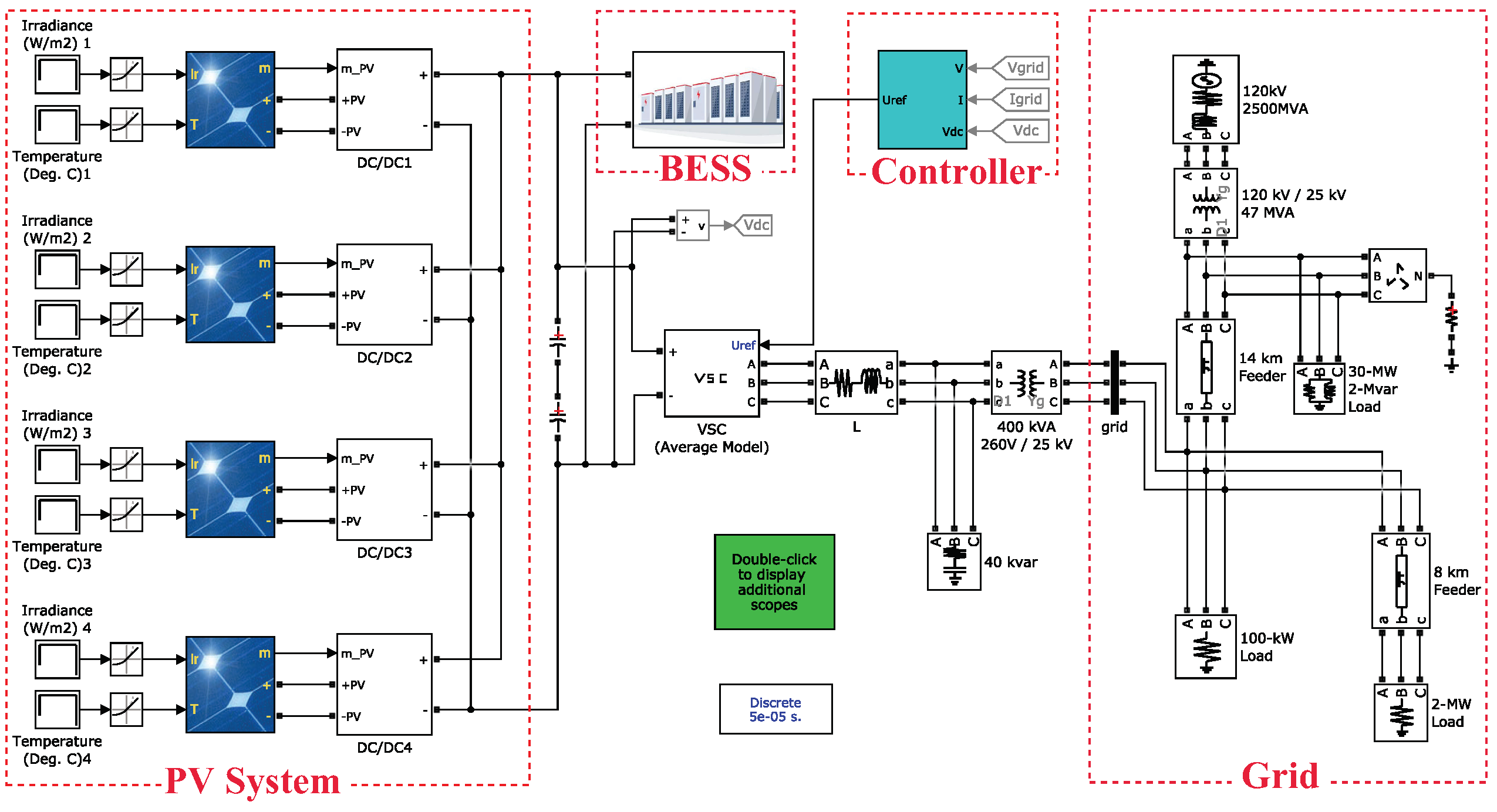
2.2. Mathematical Modeling of PV Grid-Connected Systems

The PV grid-connected system consists of four PV arrays, filter capacitors, R-L filters, inverters, and a three-phase grid. Then, the mathematical model of the grid-connected inverter is presented as below [11]:

$$\begin{array}{cc}\hfill \frac{d{i}_d}{dt}& =-\frac{R}{L}{i}_d+\omega i_q-\frac{E_d}{L}+\frac{u_{dc}}{L}{k}_d\hfill \\ \hfill \frac{d{i}_q}{dt}& =-\frac{R}{L}{i}_q-\omega i_d-\frac{E_d}{L}+\frac{u_{dc}}{L}{k}_q,\hfill \end{array}$$

(9)

where $E_d$, $E_q$, $i_d$, and $i_q$ denote the grid voltages and currents in the d-q axis, respectively; and R, L, and C represent the resistance, inductance, and capacitance of the system, respectively. $k_d$ and $k_q$ denote the switching function in the d-q axis.

On the other hand, it is acquired referring to the Kirchhoff’s Voltage and Current Laws that

$$C\frac{d{u}_{dc}}{dt}=i_0-i_{dc},$$

(10)

where $u_{dc}$ denotes the DC bus voltage, $i_0$ represents the output current of the boost circuit, and $i_{dc}$ expresses the input current of the inverter. Besides, regardless of the power loss of inverters, the following equation is provided to achieve power balance as

$$u_{dc}{i}_0=\frac{3}{2}\left(E_d{i}_d+E_q{i}_q\right),$$

(11)

where $E_q$ is considered as 0 when the system is operating at a steady state. Then, substituting (11) to (10), it can be derived further as follows:

$$\frac{d{u}_{dc}}{dt}=\frac{3E_d{i}_d}{2C{u}_{dc}}-\frac{i_{dc}}{C}.$$

(12)

To summarize, the complete mathematical model of the grid-connected inverter is described as follows [11]:

$$\begin{array}{cc}\hfill \frac{d{u}_{dc}}{dt}& =\frac{3E_d{i}_d}{2C{u}_{dc}}-\frac{i_{dc}}{C}\hfill \\ \hfill \frac{d{i}_d}{dt}& =-\frac{R}{L}{i}_d+\omega i_q-\frac{E_d}{L}+\frac{u_d}{L}\hfill \\ \hfill \frac{d{i}_q}{dt}& =-\frac{R}{L}{i}_q-\omega i_d-\frac{E_q}{L}+\frac{u_q}{L}.\hfill \end{array}$$

(13)

Since it is tough to measure the value of the system parameter accurately, the parameters could be considered uncertain during the controller design process, which is described as

$${\eta }_1=\frac{1}{C},{\eta }_2=\frac{R}{L},{\eta }_3=\frac{1}{L}.$$

(14)

Taking (14) into account, the mathematical model (13) can be rewritten as [11]

$$\begin{array}{cc}\hfill \frac{d{u}_{dc}}{dt}& ={\eta }_1\left(\frac{3E_d{i}_d}{2u_{dc}}-i_{dc}\right)\hfill \\ \hfill \frac{d{i}_d}{dt}& =-{\eta }_2{i}_d+\omega i_q-{\eta }_3{E}_d+{\eta }_3{u}_d\hfill \\ \hfill \frac{d{i}_q}{dt}& =-{\eta }_2{i}_{\mathrm{q}}-\omega i_d-{\eta }_3{E}_q+{\eta }_3{u}_q.\hfill \end{array}$$

(15)

2.3. Basic Principle of Prescribed Performance Control

In order to obtain the desired performance with high accuracy, the PPC technique is adopted in this paper by pre-setting a range for the tracking error to achieve the prescribed performance.

First, a smooth function $p\left(t\right)$: $R^{+}\to R^{+}$ is introduced to constrain the tracking error, which should be positive and monotonically decreasing and satisfy ${\lim }_{t\to \infty }p\left(t\right)=p_{\infty }>0$ [30]. Here, we choose the following function which satisfies the aforementioned conditions, namely,

$$p\left(t\right)=\left(p_0-p_{\infty }\right)e^{-lt}+p_{\infty },$$

(16)

where $p_0$, $p_{\infty }$, and l are all positive constants. Then, the defined tracking error ${\overline{z}}_1$ can be constrained within the following prescribed range as

$$-p\left(t\right)<{\overline{z}}_1\left(t\right)<p\left(t\right).$$

(17)

Considering the smooth function (16) and the error constraint (17), the amplitude and convergence rate of tracking error ${\overline{z}}_1$ will be determined by the smooth function $p\left(t\right)$ if the initial value of the defined tracking error ${\overline{z}}_1$ satisfies $0\le \left|{\overline{z}}_1\left(0\right)\right|\le p_0$.

Furthermore, when it comes to the controller design process, it is necessary to convert the constrained problem into an equivalent unconstrained one. Hence, the constrained tracking error is represented by the combination of smooth function $p\left(t\right)$ and transformation function $\zeta \left(t\right)$, that is,

$${\overline{z}}_1\left(t\right)=p\left(t\right)\zeta \left(\epsilon \left(t\right)\right),$$

(18)

where $\epsilon \left(t\right)$ is the transformation error and $\zeta \left(\epsilon \right(t\left)\right)$ should be equipped with the smooth, monotonically increasing, and reversible characteristics [30]. Notice that $\zeta \left(\epsilon \right(t\left)\right)$ is rewritten as $\zeta \left(\epsilon \right)$ for simplicity in the following contents. Apart from the above characteristics, $\zeta \left(\epsilon \right)$ ought to satisfy another two conditions, that is,

$$-1<\zeta \left(\epsilon \right)<1$$

(19)

$$\left\{\begin{array}{cc}\hfill \underset{\epsilon \to -\infty }{lim}\zeta \left(\epsilon \right)& =-1\hfill \\ \hfill \underset{\epsilon \to \infty }{lim}\zeta \left(\epsilon \right)& =1\hfill \end{array}\right.$$

(20)

Based on the above description, $\zeta \left(\epsilon \right)$ is chosen as

$$\zeta \left(\epsilon \right)=\frac{e^{\epsilon }-e^{-\epsilon }}{e^{\epsilon }+e^{-\epsilon }}.$$

(21)

Thus, the transformed error $\epsilon \left(t\right)$ is described in the following form as

$$\epsilon \left(t\right)={\zeta }^{-1}\left(\frac{{\overline{z}}_1\left(t\right)}{p\left(t\right)}\right)=\frac{1}{2}\ln \frac{{\overline{z}}_1\left(t\right)+p\left(t\right)}{p\left(t\right)-{\overline{z}}_1\left(t\right)}.$$

(22)

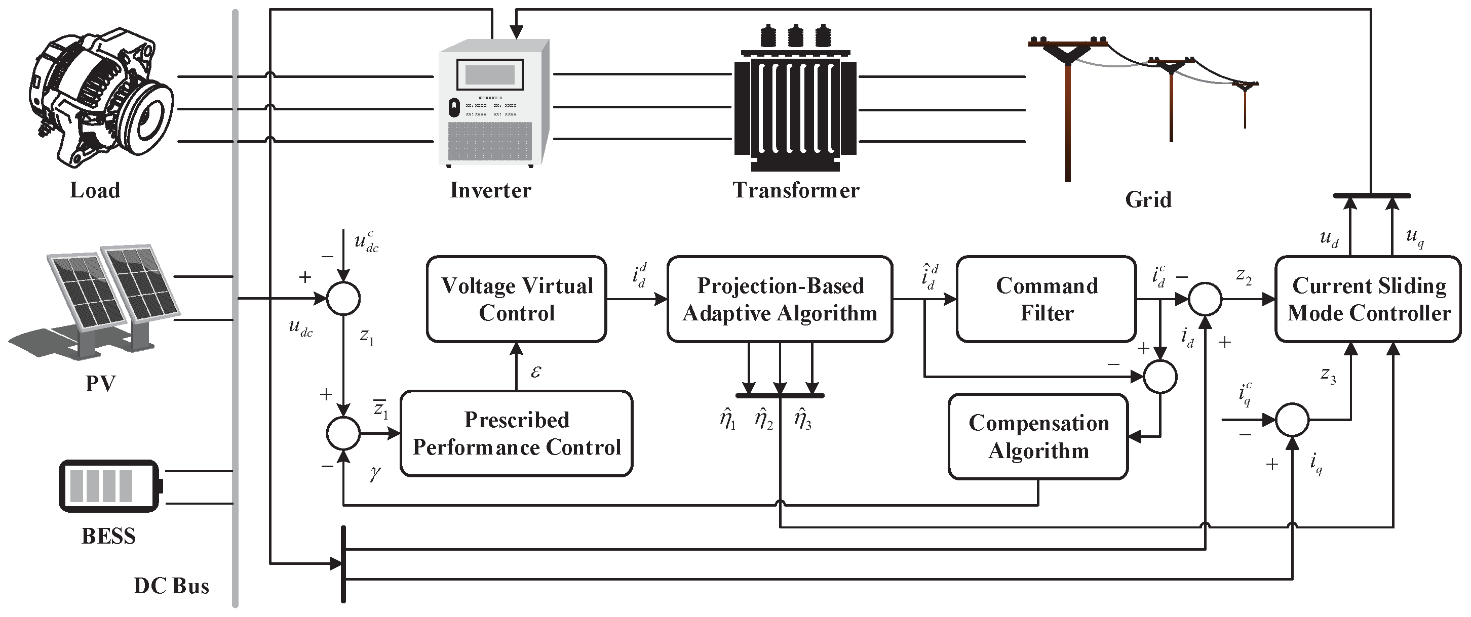
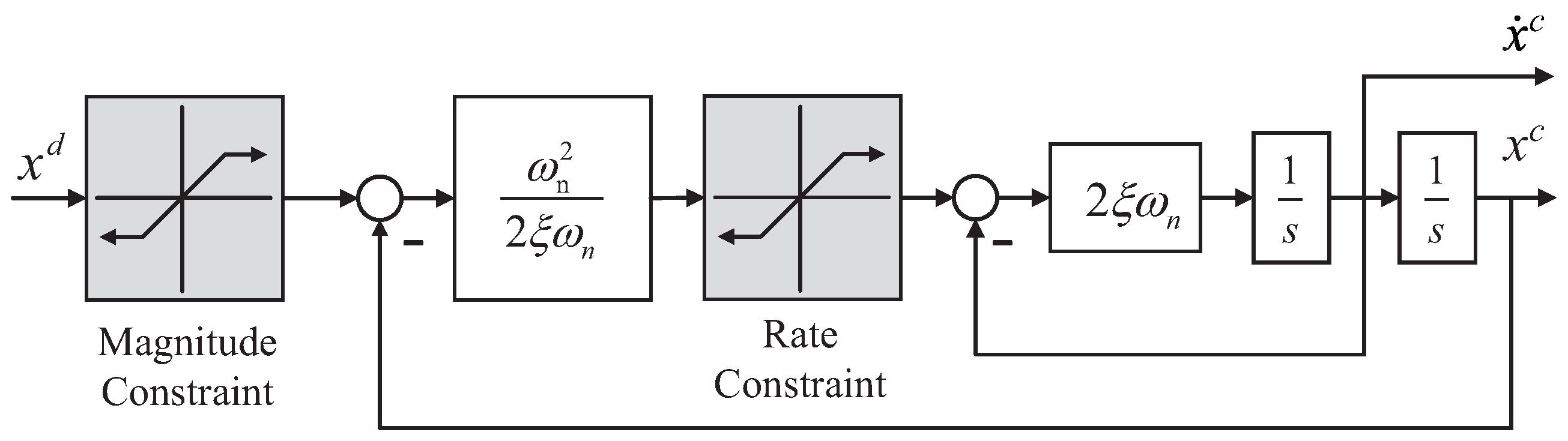
2.4. Proposed Controller Design for Grid-Connected Inverter and Stability Proof

In this section, the proposed prescribed performance-based command-filtered backstepping adaptive sliding mode controller is established to gain the stable DC-link voltage and expected power demanded by the PV grid-connected system. More specifically, the control law $u_d$ and $u_q$ are both established to track the reference current, so that the control objective can be achieved. The block of the whole control system is depicted in Figure 3 and the concrete design process is described in the following.

A series of tracking errors are defined first as follows.

$$z_1=u_{dc}-u_{dc}^c$$

(23)

$$z_2=i_d-i_d^c$$

(24)

$$z_3=i_q-i_q^c.$$

(25)

Considering that the numerous differential processes are inevitable in the controller design process due to the existence of the derivatives of virtual control signals, the command filter is employed in order to avoid the potential differential expansion, whose structure diagram is drawn in Figure 4 and dynamics are given as follows [11,22,31].

$$\left[\begin{array}{c}\hfill {\dot{q}}_1\\ \hfill {\dot{q}}_2\end{array}\right]=\left[\begin{array}{c}{q}_2\hfill \\ 2\xi {\omega }_n\left[S_R\left(\frac{{\omega }_n^2}{2\xi {\omega }_n}\left(S_A\left(u\right)-q_1\right)\right)-q_2\right],\hfill \end{array}\right]$$

(26)

where

$$\begin{array}{c}\hfill \left[\begin{array}{c}{q}_1\hfill \\ q_2\hfill \end{array}\right]=\left[\begin{array}{c}{x}^c\\ {\dot{x}}^c\end{array}\right],u=x^d,\end{array}$$

(27)

and other parameters are defined as follows: ${\omega }_n$ and $\xi$ are the bandwidth and damping of the command filter; and $S_A(.)$ and $S_R(.)$ are the amplitude and magnitude constraint, respectively.

Since the filter error is inevitable during the filtering process, a corresponding compensated tracking error is defined as

$${\overline{z}}_1=z_1-{\gamma }_1,$$

(28)

where ${\gamma }_1$ denotes the compensation signal with respect to the filter error, and has the following form:

$${\dot{\gamma }}_1=-\beta {\gamma }_1+\frac{3E_d{\eta }_1}{2u_{dc}}\left(i_d^c-i_d^d\right),$$

(29)

where $\beta >0$ is the compensation coefficient. Combining (15), (28) and (29), we can achieve the further representation of ${\dot{\overline{z}}}_1$ as follows.

$${\dot{\overline{z}}}_1=\frac{3E_d{i}_d{\eta }_1}{2u_{dc}}-{\eta }_1{i}_{dc}-{\dot{u}}_{dc}^c+\beta {\gamma }_1-\frac{3E_d{\eta }_1}{2u_{dc}}{i}_d^c+\frac{3E_d{\eta }_1}{2u_{dc}}{i}_d^d.$$

(30)

Meanwhile, according to (22), the derivative of the transformed error $\epsilon$ is obtained as

$$\dot{\epsilon }=\frac{\partial {\zeta }^{-1}}{\partial \left({\overline{z}}_1/p\right)}\frac{1}{p}\left({\dot{\overline{z}}}_1-\frac{\dot{p}{\overline{z}}_1}{p}\right)=r({\dot{\overline{z}}}_1-\upsilon ),$$

(31)

where $r=\frac{p}{p^2-{\overline{z}}_1^2}$ and $\upsilon =\frac{\dot{p}{\overline{z}}_1}{p}$ is defined for simplicity. Referring to the characteristics of the smooth function $p\left(t\right)$ and transformation function $\zeta \left(t\right)$, it can be deduced that $r>0$.

Then, the first Lyapunov function is given as

$$V_1=\frac{1}{2}{\epsilon }^2.$$

(32)

Taking (30) and (31) into account, the further relationship can be obtained as follows.

$${\dot{V}}_1=\epsilon r\left(\frac{3E_d{i}_d{\eta }_1}{2u_{dc}}-{\eta }_1{i}_{dc}-{\dot{u}}_{dc}^c+\beta {\gamma }_1-\frac{3E_d{\eta }_1}{2u_{dc}}{i}_d^c+\frac{3E_d{\eta }_1}{2u_{dc}}{i}_d^d-\upsilon \right),$$

(33)

and the virtual control law is selected as follows:

$$i_d^d=\frac{2u_{dc}}{3E_d{\eta }_1}\left({\eta }_1{i}_{dc}+{\dot{u}}_{dc}^c-\beta {\gamma }_1+\upsilon -k_1\epsilon \right),$$

(34)

where $k_1$ is a positive constant. Substituting the virtual controller (34) into (33), it is derived as

$${\dot{V}}_1=-k_{1}r{\epsilon }^2+\frac{3E_d{\eta }_1}{2u_{dc}}\epsilon r{z}_2.$$

(35)

Notice that the parameter ${\eta }_1$ is unknown, and an estimation value ${\widehat{\eta }}_1$ is used here, whose adaptive algorithm would be given thereinafter, and the virtual controller and compensation signal are rewritten as follows, respectively.

$${\widehat{i}}_d^d=\frac{2u_{dc}}{3E_d{\widehat{\eta }}_1}\left({\widehat{\eta }}_1{i}_{dc}+{\dot{u}}_{dc}^c-\beta {\gamma }_1+\upsilon -k_1\epsilon \right);$$

(36)

$${\dot{\gamma }}_1=-k_1{\gamma }_1+\frac{3E_d{\widehat{\eta }}_1}{2u_{dc}}\left(i_d^c-{\widehat{i}}_d^d\right).$$

(37)

Considering the robustness of the sliding mode control (SMC) method with respect to the disturbance and unknown parameters, SMC is employed in this paper for current control. Moreover, the integral SMC can eliminate the arrival phase by adjusting the reasonable initial state of the integrator so that the robustness can be improved. Thus, the integral sliding surfaces are defined based on the current tracking errors of d-q axis, as follows [11].

$$S_2=z_2+{\tau }_2{\int }_0^t{z}_{2}dt$$

(38)

$$S_3=z_3+{\tau }_3{\int }_0^t{z}_{3}dt,$$

(39)

where ${\tau }_2$ and ${\tau }_3$ are both positive coefficients of the integral sliding surface.

Then, another Lyapunov function composed of the transformation error, sliding surfaces, and adaptive parameters is defined as

$$V_2=V_1+\frac{1}{2}\left({S_2}^2+{S_3}^2+\frac{{\tilde{\eta }}_1^2}{{\lambda }_1}+\frac{{\tilde{\eta }}_2^2}{{\lambda }_2}+\frac{{\tilde{\eta }}_3^2}{{\lambda }_3}\right),$$

(40)

where ${\lambda }_1$, ${\lambda }_2$, and ${\lambda }_3$ are the adaptive gains; ${\tilde{\eta }}_1={\eta }_1-{\widehat{\eta }}_1$, ${\tilde{\eta }}_2={\eta }_2-{\widehat{\eta }}_2$ and ${\tilde{\eta }}_3={\eta }_3-{\widehat{\eta }}_3$ are the estimation errors of unknown parameters. In light of (35), the derivation of $V_2$ is obtained as follows:

$${\dot{V}}_2=-k_{1}r{\epsilon }^2+\frac{3E_d{\eta }_1}{2u_{dc}}\epsilon r{z}_2+S_2{\dot{S}}_2+S_3{\dot{S}}_3-\frac{{\tilde{\eta }}_1}{{\lambda }_1}{\dot{\widehat{\eta }}}_1-\frac{{\tilde{\eta }}_2}{{\lambda }_2}{\dot{\widehat{\eta }}}_2-\frac{{\tilde{\eta }}_3}{{\lambda }_3}{\dot{\widehat{\eta }}}_3,$$

(41)

where ${\dot{S}}_2$ is derived based on (15), (24) and (38) as

$$\begin{array}{cc}\hfill {\dot{S}}_2& ={\dot{z}}_2+{\tau }_2{z}_2\hfill \\ \hfill & =-{\eta }_2{i}_d+\omega i_q+{\eta }_3\left(u_d-E_d\right)-{\dot{i}}_d^c+{\tau }_2{z}_2\hfill \\ \hfill & =-{\widehat{\eta }}_2{i}_d-{\tilde{\eta }}_2{i}_d+\omega i_q+{\widehat{\eta }}_3\left(u_d-E_d\right)+{\tilde{\eta }}_3\left(u_d-E_d\right)-{\dot{i}}_d^c+{\tau }_2{z}_2,\hfill \end{array}$$

(42)

and ${\dot{S}}_3$ is derived based on (15), (25) and (39) as

$$\begin{array}{cc}\hfill {\dot{S}}_3& ={\dot{z}}_3+{\tau }_3{z}_3\hfill \\ \hfill & =-{\eta }_2{i}_q-\omega i_d+{\eta }_3\left(u_q-E_q\right)-{\dot{i}}_q^c+{\tau }_3{z}_3\hfill \\ \hfill & =-{\widehat{\eta }}_2{i}_q-{\tilde{\eta }}_2{i}_q-\omega i_d+{\widehat{\eta }}_3\left(u_q-E_q\right)+{\tilde{\eta }}_3\left(u_q-E_q\right)-{\dot{i}}_q^c+{\tau }_3{z}_3.\hfill \end{array}$$

(43)

Through substitution and simplification, the results can be figured out as follows:

$$\begin{array}{cc}\hfill {\dot{V}}_2=& -k_{1}r{\epsilon }^2+S_2\left(\frac{3E_d{\widehat{\eta }}_1\epsilon r{z}_2}{2u_{dc}{S}_2}-{\widehat{\eta }}_2{i}_d+\omega i_q+{\widehat{\eta }}_3\left(u_d-E_d\right)-{\dot{i}}_d^c+{\tau }_2{z}_2\right)\hfill \\ \hfill & +S_3\left(-{\widehat{\eta }}_2{i}_q-\omega i_d+{\widehat{\eta }}_3\left(u_q-E_q\right)-{\dot{i}}_q^c+{\tau }_3{z}_3\right)\hfill \\ \hfill & +{\tilde{\eta }}_1\left(\frac{3E_d\epsilon r{z}_2}{2u_{dc}}-\frac{{\dot{\widehat{\eta }}}_1}{{\lambda }_1}\right)+{\tilde{\eta }}_2\left(-\frac{{\dot{\widehat{\eta }}}_2}{{\lambda }_2}-S_2{i}_d-S_3{i}_q\right)\hfill \\ \hfill & +{\tilde{\eta }}_3\left(-\frac{{\dot{\widehat{\eta }}}_3}{{\lambda }_3}+S_2\left(u_d-E_d\right)+S_3\left(u_q-E_q\right)\right).\hfill \end{array}$$

(44)

In order to achieve the asymptotical stability of the system, the projection-based adaptive law is established to eliminate the influence of ${\eta }_1$, ${\eta }_2$, and ${\eta }_3$, which is represented as

$$\begin{array}{cc}\hfill {\dot{\widehat{\eta }}}_1& ={\lambda }_1\mathrm{Proj}\left({\widehat{\eta }}_1,\frac{3E_d\epsilon r{z}_2}{2u_{dc}}\right)\hfill \\ \hfill {\dot{\widehat{\eta }}}_2& ={\lambda }_2\mathrm{Proj}\left({\widehat{\eta }}_2,-S_2{i}_d-S_3{i}_q\right)\hfill \\ \hfill {\dot{\widehat{\eta }}}_3& ={\lambda }_3\mathrm{Proj}\left({\widehat{\eta }}_3,S_2\left(u_d-E_d\right)+S_3\left(u_q-E_q\right)\right),\hfill \end{array}$$

(45)

where Proj ($·,·$) represents the projection operator [32]. The projection-based adaptive algorithm is employed here to ensure the boundedness of the estimated parameters, and the following relationship can be obtained as

$$\begin{array}{c}{\tilde{\eta }}_1\left[\frac{3E_d\epsilon r{z}_2}{2u_{dc}}-\mathrm{Proj}\left({\widehat{\eta }}_1,\frac{3E_d\epsilon r{z}_2}{2u_{dc}}\right)\right]\le 0\\ {\tilde{\eta }}_2\left[-S_2{i}_d-S_3{i}_q-\mathrm{Proj}\left({\widehat{\eta }}_2,-S_2{i}_d-S_3{i}_q\right)\right]\le 0\\ {\tilde{\eta }}_3\left[S_2\left(u_d-E_d\right)+S_3\left(u_q-E_q\right)-\mathrm{Proj}\left({\widehat{\eta }}_3,S_2\left(u_d-E_d\right)+S_3\left(u_q-E_q\right)\right)\right]\le 0.\end{array}$$

Hence, we can get the following inequality related to ${\dot{V}}_2$ as

$$\begin{array}{cc}\hfill {\dot{V}}_2\le & -k_{1}r{\epsilon }^2+S_2\left(\frac{3E_d{\widehat{\eta }}_1\epsilon r{z}_2}{2u_{dc}{S}_2}-{\widehat{\eta }}_2{i}_d+\omega i_q+{\widehat{\eta }}_3\left(u_d-E_d\right)-{\dot{i}}_d^c+{\tau }_2{z}_2\right)\hfill \\ \hfill & +S_3\left(-{\widehat{\eta }}_2{i}_q-\omega i_d+{\widehat{\eta }}_3\left(u_q-E_q\right)-{\dot{i}}_q^c+{\tau }_3{z}_3\right).\hfill \end{array}$$

(46)

With the aim of guaranteeing the asymptotical stability of the system, ${\dot{V}}_2$ ought to remain non-positive, that is, ${\dot{V}}_2\le 0$. As a result, the following saturation function is used here for stability.

$$\begin{array}{cc}\hfill -k_2\mathrm{Sat}\left(S_2\right)& =\frac{3E_d{\widehat{\eta }}_1\epsilon r{z}_2}{2u_{dc}{S}_2}-{\widehat{\eta }}_2{i}_d+\omega i_q+{\widehat{\eta }}_3\left(u_d-E_d\right)-{\dot{i}}_d^c+{\tau }_2{z}_2\hfill \\ \hfill -k_3\mathrm{Sat}\left(S_3\right)& =-{\widehat{\eta }}_2{i}_q-\omega i_d+{\widehat{\eta }}_3\left(u_q-E_q\right)-{\dot{i}}_q^c+{\tau }_3{z}_3,\hfill \end{array}$$

(47)

where $k_2$ and $k_3$ are both positive constants, and $\mathrm{Sat}(·)$ denotes the saturation function, which is given as follows.

$$\begin{array}{c}\hfill \mathrm{Sat}\left(x\right)=\left\{\begin{array}{c}1,x>\phi \hfill \\ x/\phi ,\left|x\right|\le \phi \hfill \\ -1,x<-\phi \hfill \end{array}\right.\end{array}$$

(48)

where $\phi \in (0,0.5]$ is the sliding layer. In conclusion, the control law $u_d$ and $u_q$ can be obtained in the following.

$$\begin{array}{cc}\hfill u_d& =-\frac{1}{{\widehat{\eta }}_3}\left(\frac{3E_d{\widehat{\eta }}_1\epsilon r{z}_2}{2u_{dc}{S}_2}-{\widehat{\eta }}_2{i}_d+\omega i_q-{\widehat{\eta }}_3{E}_d-{\dot{i}}_d^c+{\tau }_2{z}_2+k_2\mathrm{Sat}\left(S_2\right)\right)\hfill \\ \hfill u_q& =-\frac{1}{{\widehat{\eta }}_3}\left(-{\widehat{\eta }}_2{i}_q-\omega i_d-{\widehat{\eta }}_3{E}_q-{\dot{i}}_q^c+{\tau }_3{z}_3+k_3\mathrm{Sat}\left(S_3\right)\right).\hfill \end{array}$$

(49)

Under the proposed control law (49), the inequality (46) can be further described as

$${\dot{V}}_2\le -k_{1}r{\epsilon }^2-k_2{S}_2\mathrm{Sat}\left(S_2\right)-k_3{S}_3\mathrm{Sat}\left(S_3\right)\le 0.$$

(50)

Obviously, ${\dot{V}}_2=0$ holds only if $\left[\epsilon ,S_2,S_3\right]=[0,0,0]$. Considering the variation of the environmental situation, the output power generated by PV fluctuates constantly, which leads to the fluctuation of the DC bus voltage. That is to say, the voltage tracking error and sliding mode surfaces would not always be zero, which indicates that ${\dot{V}}_2$ would not always be zero. Therefore, the system is proved asymptotically stable based on the Lyapunov stability criterion and LaSalle’s invariance principle.

3. Results and Discussion

In this section, the performance of the designed controller is simulated in the MATLAB/Simulink environment and the simulation model is shown in Figure 5. Considering that the environment varies constantly, including solar irradiance and temperature, which would have an influence on the stable operation of the PV grid-connected system and lead to the power fluctuation, the distributed PV arrays under variable conditions are integrated for power generation. it is worth noting that four photovoltaic arrays, which are not far away from each other share the same set of environmental parameters including the solar irradiation and temperature, which are both shown in Figure 6a, and the external characteristics of each PV array, including output voltage, current, and power are shown in Figure 6b–d, respectively. Under the environment, the proposed controller is applied to the system for stable operation. The corresponding parameters of the PV grid-connected system and controller are both shown in

Table 2. The parameters of the control system.

Classification	Parameter	Value	Parameter	Value	Parameter	Value
	R	1 m$\Omega$	$R_1,R_2,R_3,R_4$	5 m$\Omega$	$P_g$	400 kW
PV grid-connected system	L	45 $\mathsf{\mu }$H	$L_1,L_2,L_3,L_4$	5 mH	f	60 Hz
	C	50 mF	$C_1,C_2,C_3,C_4$	0.1 mF	$u_{dc}$	500 V
	$p_0$	250	$p_{\infty }$	5	l	1.5
	$k_1$	8000	$k_2$	60,000	$k_3$	80,000
Proposed controller	${\lambda }_1$	0.1	${\lambda }_2$	0.1	${\lambda }_3$	0.1
	${\tau }_2$	3	${\tau }_3$	3	$\beta$	0.9
	$\varphi$	0.5	${\omega }_n$	300	$\xi$	0.1

.

As to the parameter adjustment of the proposed control strategy, the prescribed performance parameters rank first owing to their strong constraint on the tracking error. The initial value of the performance function $p_0$ exhibits great importance at the beginning of the system operation. Considering the inevitable response time in initial stage of the controller operation, $p_0$ shall be set relatively large, yet a too-large $p_0$ would lead to large initial overshoot. Besides, l regulates the convergence rate of the tracking error to some extent, and $p_{\infty }$ shows its effectiveness on the tracking error at the stable state. Hence, an appropriate performance function would be beneficial to the control performance. In terms of other parameters, they shall be adjusted according to the tracking error variation and some certain performance variation; for instance, the adaptive coefficient shall be adjusted in view of the estimation error of the adaptive parameters. Based on the adjusted parameters, the simulation results are given and the concrete analysis is provided as follows.

The concrete objectives of the control performance are listed as follows: The tracking error shall be constrained within ±2% and the power fluctuation shall be limited no more than ±5% at the stable state. The power demanded by grid was 400 kW, yet the maximum output power of all the PV arrays is less than 400 kW at the beginning, which brings about 30% power fluctuation. Therefore, in order to maintain power balance, the BESS needs to be taken into account and introduced in 0.5 s. The power transmission performance of each module in the power grid is shown in Figure 7. As is seen, there exists about 30% power fluctuation when the BESS is absent from the grid-connected system before 0.5 s, and the introduction of BESS compensates for the power difference since 0.5s, which contributes to the relatively stable and smooth power delivered to the grid with no more than 5% fluctuation. Besides, the output power under the proposed controller is free of overshoot and provided with a quick response.

Moreover, the DC bus voltage tracking performance is given in Figure 8. It can be found that the bus voltage under the proposed controller arrives at 510 V and converges to the reference within nearly 0.01 s at the beginning. Then, the voltage is maintained at 500.5 V under the control of the proposed strategy, while the one under CBC fluctuates at 502 V. Besides, the performance difference can be more clearly observed when BESS is introduced, namely, the fluctuation caused by BESS under the proposed controller appears little, while the one of CBC reaches 4 V, which indicates the bus voltage under the proposed controller has little fluctuation, higher convergence speed, and more precise tracking performance than the one under CBC. In order to show the effect more intuitively, the voltage tracking error is depicted in Figure 9. It indicates that the introduction of BESS brings about little overshoot under the proposed controller, yet causes large overshoot under CBC. Furthermore, the voltage error with the proposed controller holds within the performance range owing to the prescribed performance technique, which further validates the advantages of the proposed controller.

Figure 10 presents the estimation performance of the adaptive parameters. It can be found that the adaptive parameters own slow-varying curves, which correspond with their characteristics. Besides, Figure 11 shows the performance of a three-phase voltage and current at the grid side with the partial enlarged drawing. It is vividly seen that the output voltage and current of the inverter own smooth variation curves with little distortion, which indicates how the designed controller can still inject a great sinusoidal current into the grid. In addition, Figure 11c also presents the total harmonic distortion (THD) of the grid current under the proposed controller with the value of 1.88%. In contrast, the grid current is more harmonic when CBC is utilized, as shown in Figure 11d. In this case, the THD value is 2.38%. Consequently, it can proved that the proposed controller is effective for the PV grid-connected system and possesses better performance with little overshoot, a quicker response, higher accuracy, and being less harmonic than CBC.

4. Conclusions

In this paper, a novel command-filtered adaptive backstepping control strategy with a prescribed performance technique was proposed to control the active power of the PV grid-connected system. The concrete conclusions could be further drawn according to the results as follows.

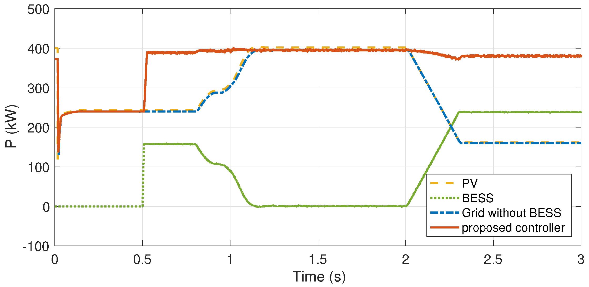
• The proposed control strategy exhibits great performance for power and voltage control of the PV grid-connected system with unknown system parameters and constantly variable environmental conditions.
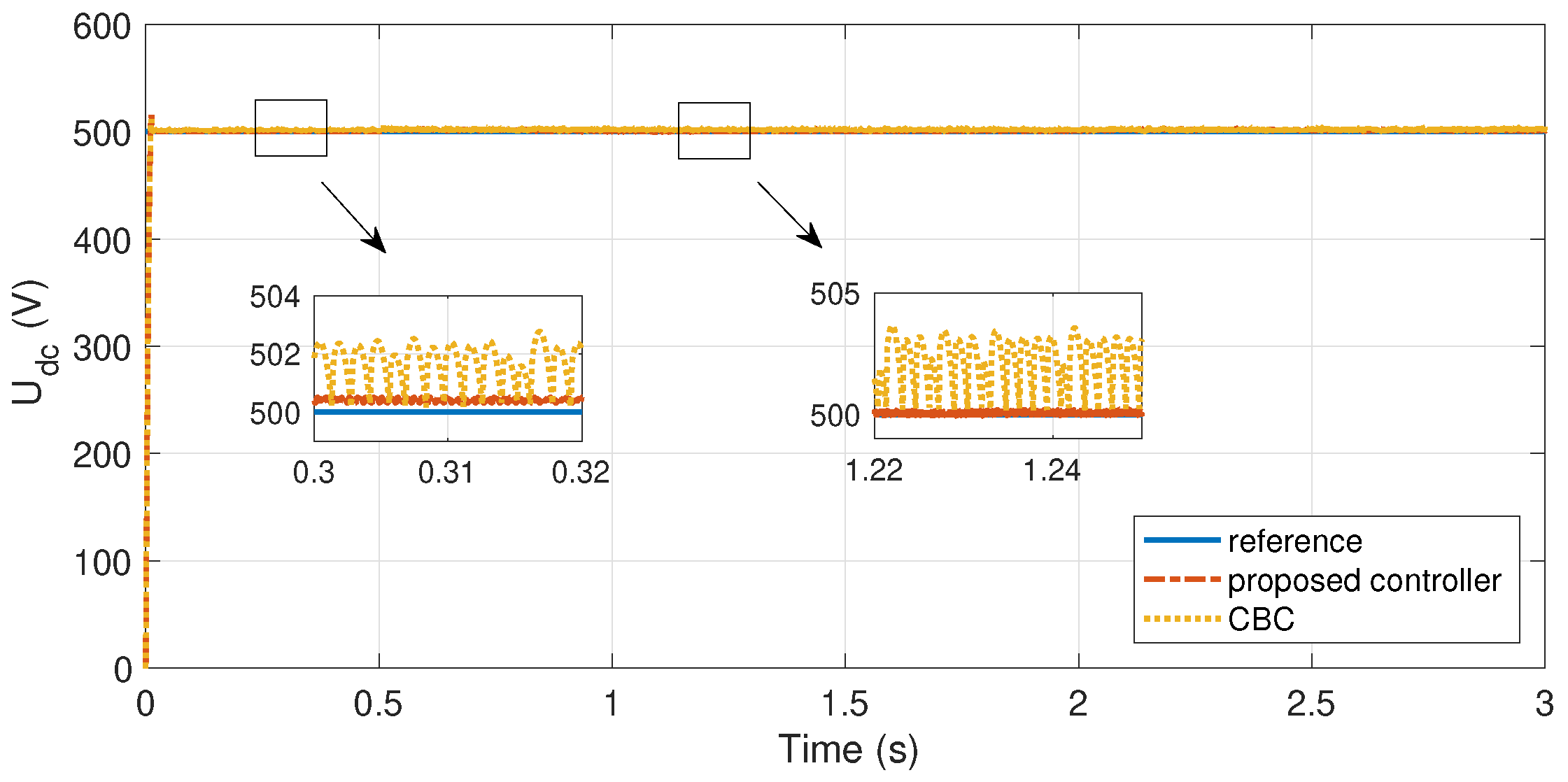
• The DC bus voltage tracking error is constrained within the preset range owing to the introduction of prescribed performance technique, which guarantees high tracking precision and constitutes to the stable operation of the system.
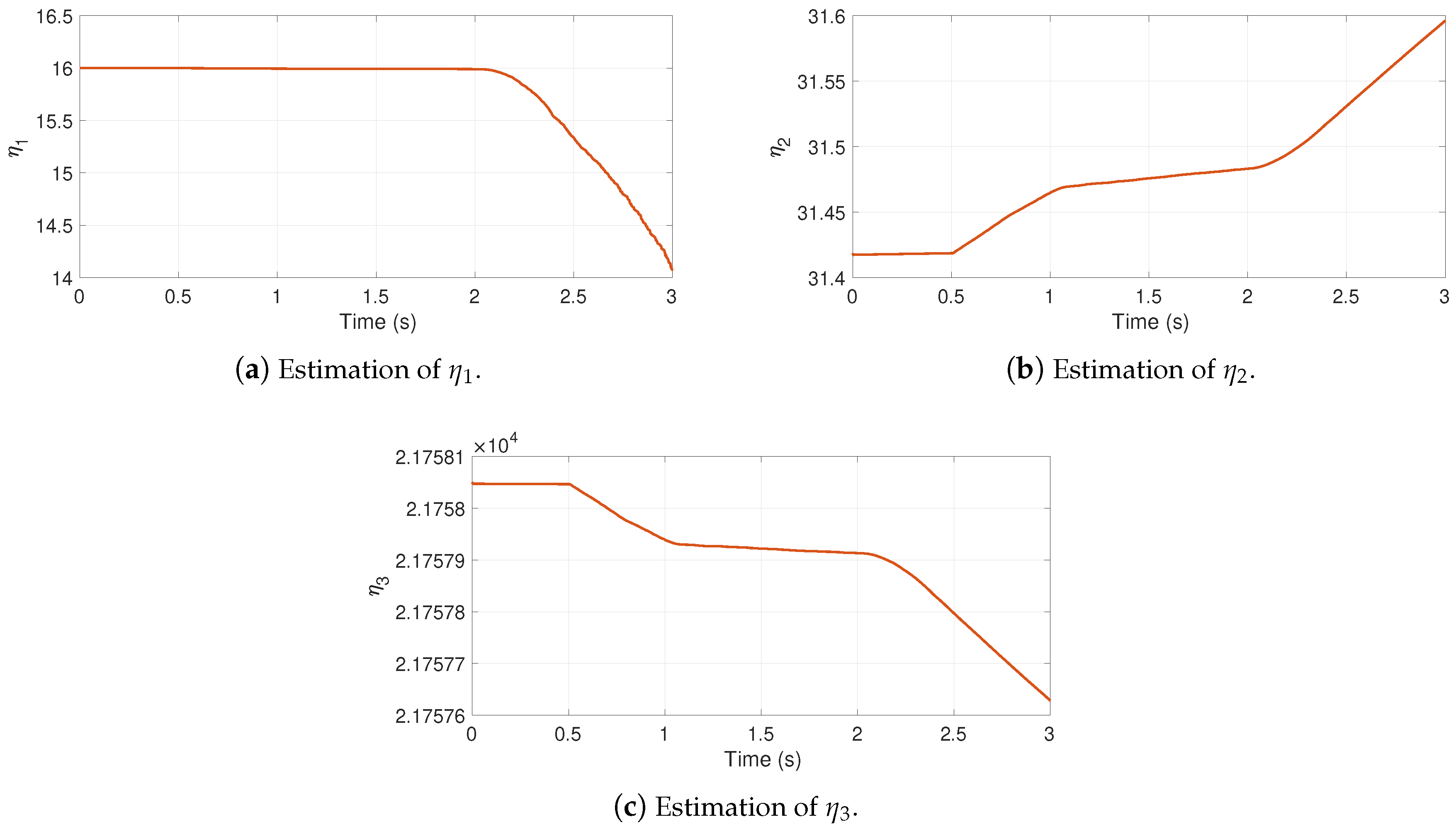
• The introduced projection-based adaptive law provides accurate estimation for system parameters, which is more in line with the actual system.
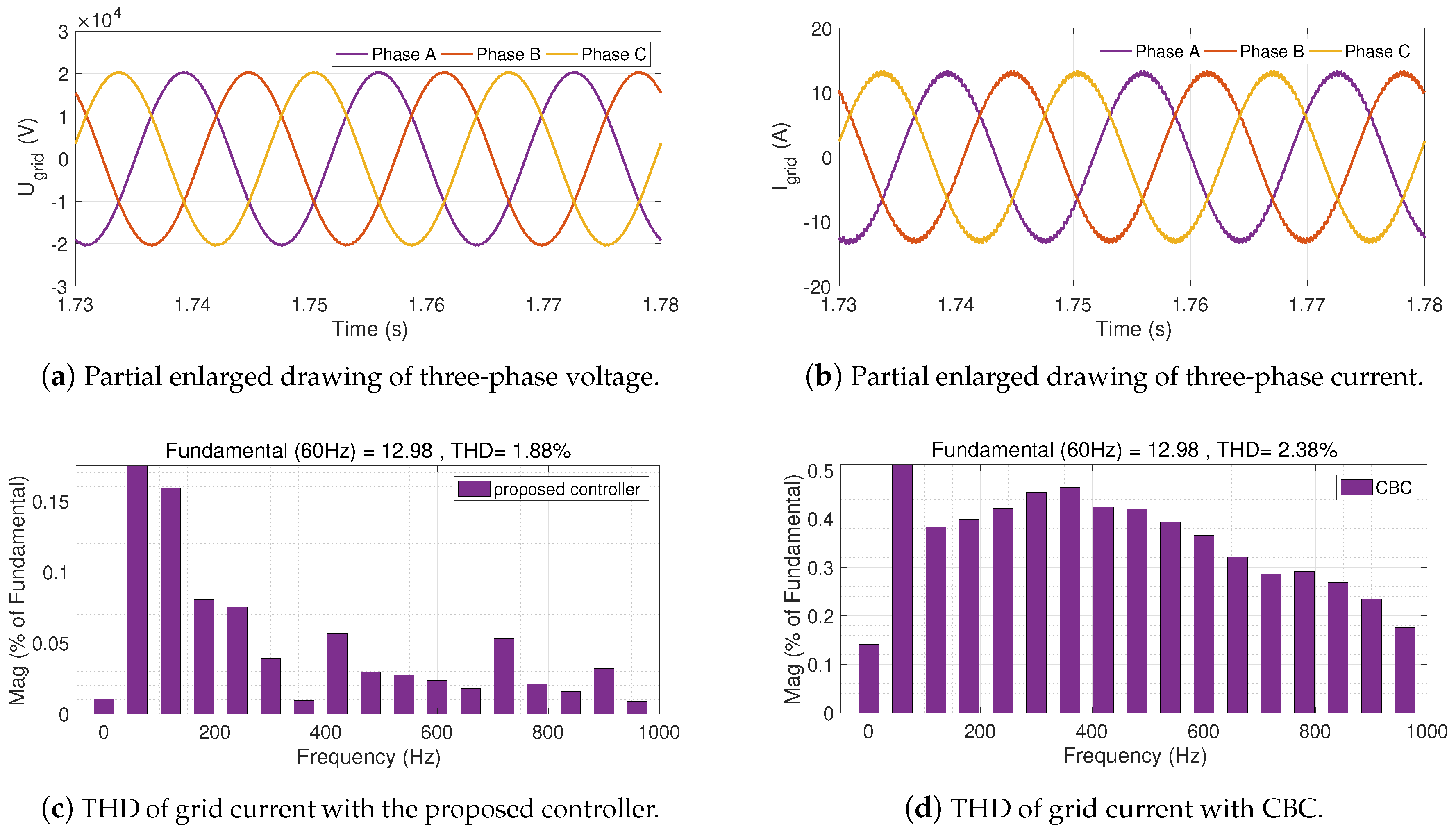
• Comparing with CBC, the prescribed performance-based control strategy owns more stable power delivery and voltage with little fluctuation, which shows better static and dynamic performance of the proposed controller.

In the future, the semi-physical experiment platform of a small-scale PV grid-connected system shall be established to further validate the effectiveness and practicability of the proposed controller.

References

1. Kouro, S.; Leon, J.I.; Vinnikov, D.; Franquelo, L.G. Grid-connected photovoltaic systems: An overview of recent research and emerging PV converter technology. IEEE Ind. Electron. Mag. 2015, 9, 47–61. [Google Scholar] [CrossRef]
2. Eltawil, M.A.; Zhao, Z. Grid-connected photovoltaic power systems: Technical and potential problems—A review. Renew. Sustain. Energy Rev. 2010, 14, 112–129. [Google Scholar] [CrossRef]
3. Yang, B.; Li, W.; Zhao, Y.; He, X. Design and analysis of a grid-connected photovoltaic power system. IEEE Trans. Power Electron. 2010, 25, 992–1000. [Google Scholar] [CrossRef]
4. Li, S.; Wei, Z.; Ma, Y. Fuzzy load-shedding strategy considering photovoltaic output fluctuation characteristics and static voltage stability. Energies 2018, 11, 779. [Google Scholar] [CrossRef] [Green Version]
5. Liserre, M.; Teodorescu, R.; Blaabjerg, F. Stability of photovoltaic and wind turbine grid-connected inverters for a large set of grid impedance values. IEEE Trans. Power Electron. 2006, 21, 263–272. [Google Scholar] [CrossRef]
6. Li, Y.; Ishikawa, M. An efficient reactive power control method for power network systems with solar photovoltaic generators using sparse optimization. Energies 2017, 10, 696. [Google Scholar] [CrossRef] [Green Version]
7. Zhang, Q.; Zhou, L.; Mao, M.; Xie, B.; Zheng, C. Power quality and stability analysis of large-scale grid-connected photovoltaic system considering non-linear effects. IET Power Electron. 2018, 11, 1739–1747. [Google Scholar] [CrossRef]
8. Mahmud, M.A.; Pota, H.; Hossain, M. Dynamic stability of three-phase grid-connected photovoltaic system using zero dynamic design approach. IEEE J. Photovoltaics 2012, 2, 564–571. [Google Scholar] [CrossRef]
9. Yıldıran, N.; Tacer, E. A new approach to H-infinity control for grid-connected inverters in photovoltaic generation systems. Electr. Power Components Syst. 2019, 47, 1413–1422. [Google Scholar] [CrossRef]
10. Zhu, Y.; Fei, J. Adaptive global fast terminal sliding mode control of grid-connected photovoltaic system using fuzzy neural network approach. IEEE Access 2017, 5, 9476–9484. [Google Scholar] [CrossRef]
11. Xu, D.; Wang, G.; Yan, W.; Yan, X. A novel adaptive command-filtered backstepping sliding mode control for PV grid-connected system with energy storage. Sol. Energy 2019, 178, 222–230. [Google Scholar] [CrossRef] [Green Version]
12. Farrell, J.A.; Polycarpou, M.; Sharma, M.; Dong, W. Command filtered backstepping. IEEE Trans. Autom. Control 2009, 54, 1391–1395. [Google Scholar] [CrossRef]
13. Yu, J.; Shi, P.; Zhao, L. Finite-time command filtered backstepping control for a class of nonlinear systems. Automatica 2018, 92, 173–180. [Google Scholar] [CrossRef]
14. Shen, Q.; Shi, P. Distributed command filtered backstepping consensus tracking control of nonlinear multiple-agent systems in strict-feedback form. Automatica 2015, 53, 120–124. [Google Scholar] [CrossRef]
15. Cui, G.; Xu, S.; Lewis, F.L.; Zhang, B.; Ma, Q. Distributed consensus tracking for non-linear multi-agent systems with input saturation: A command filtered backstepping approach. IET Control Theory Appl. 2016, 10, 509–516. [Google Scholar] [CrossRef]
16. Yu, J.; Zhao, L.; Yu, H.; Lin, C.; Dong, W. Fuzzy finite-time command filtered control of nonlinear systems with input saturation. IEEE Trans. Cybern. 2017, 48, 2378–2387. [Google Scholar]
17. Pan, Y.; Wang, H.; Li, X.; Yu, H. Adaptive command-filtered backstepping control of robot arms with compliant actuators. IEEE Trans. Control Syst. Technol. 2017, 26, 1149–1156. [Google Scholar] [CrossRef]
18. Jin, Z.; Zhang, W.; Liu, S.; Gu, M. Command-filtered backstepping integral sliding mode control with prescribed performance for ship roll stabilization. Appl. Sci. 2019, 9, 4288. [Google Scholar] [CrossRef] [Green Version]
19. Ren, H.; Deng, G.; Hou, B.; Wang, S.; Zhou, G. Finite-time command filtered backstepping algorithm-based pitch angle tracking control for wind turbine hydraulic pitch systems. IEEE Access 2019, 7, 135514–135524. [Google Scholar] [CrossRef]
20. Choi, I.H.; Bang, H.C. Adaptive command filtered backstepping tracking controller design for quadrotor unmanned aerial vehicle. Proc. Inst. Mech. Eng. Part J. Aerosp. Eng. 2012, 226, 483–497. [Google Scholar] [CrossRef]
21. Zhao, S.; Dong, W.; Farrell, J.A. Quaternion-based trajectory tracking control of VTOL-UAVs using command filtered backstepping. In Proceedings of the 2013 American Control Conference, Washington, DC, USA, 17–19 June 2013; IEEE: Piscataway, NJ, USA, 2013; pp. 1018–1023. [Google Scholar]
22. Bechlioulis, C.P.; Rovithakis, G.A. Robust adaptive control of feedback linearizable MIMO nonlinear systems with prescribed performance. IEEE Trans. Autom. Control 2008, 53, 2090–2099. [Google Scholar] [CrossRef]
23. Na, J.; Chen, Q.; Ren, X.; Guo, Y. Adaptive prescribed performance motion control of servo mechanisms with friction compensation. IEEE Trans. Ind. Electron. 2013, 61, 486–494. [Google Scholar] [CrossRef]
24. Huang, Y.; Na, J.; Wu, X.; Liu, X.; Guo, Y. Adaptive control of nonlinear uncertain active suspension systems with prescribed performance. ISA Trans. 2015, 54, 145–155. [Google Scholar] [CrossRef]
25. Kostarigka, A.K.; Doulgeri, Z.; Rovithakis, G.A. Prescribed performance tracking for flexible joint robots with unknown dynamics and variable elasticity. Automatica 2013, 49, 1137–1147. [Google Scholar] [CrossRef]
26. Zhou, Q.; Li, H.; Wang, L.; Lu, R. Prescribed performance observer-based adaptive fuzzy control for nonstrict-feedback stochastic nonlinear systems. IEEE Trans. Syst. Man Cybern. Syst. 2017, 48, 1747–1758. [Google Scholar] [CrossRef]
27. Qiu, J.; Sun, K.; Wang, T.; Gao, H. Observer-based fuzzy adaptive event-triggered control for pure-feedback nonlinear systems with prescribed performance. IEEE Trans. Fuzzy Syst. 2019, 27, 2152–2162. [Google Scholar] [CrossRef]
28. Belhachat, F.; Larbes, C. Modeling, analysis and comparison of solar photovoltaic array configurations under partial shading conditions. Sol. Energy 2015, 120, 399–418. [Google Scholar] [CrossRef]
29. Dhoke, A.; Sharma, R.; Saha, T.K. An approach for fault detection and location in solar PV systems. Sol. Energy 2019, 194, 197–208. [Google Scholar] [CrossRef]
30. Liu, D.; Yang, G.H. Data-driven adaptive sliding mode control of nonlinear discrete-time systems with prescribed performance. IEEE Trans. Syst. Man Cybern. Syst.s 2019, 49, 2598–2604. [Google Scholar] [CrossRef]
31. Jiang, B.; Xu, D.; Shi, P.; Lim, C.C. Adaptive neural observer-based backstepping fault tolerant control for near space vehicle under control effector damage. IET Control Theory Appl. 2014, 8, 658–666. [Google Scholar] [CrossRef]
32. Chen, H.; Wang, H. Numerical simulation for conservative fractional diffusion equations by an expanded mixed formulation. J. Comput. Appl. Math. 2016, 296, 480–498. [Google Scholar] [CrossRef]
Figure 1. Circuit topology of a PV cell.
Sustainability 12 07429 g001
Figure 2. Configuration of the PV system.
Sustainability 12 07429 g002
Figure 3. Control block of the proposed controller in the PV grid-connected system.
Sustainability 12 07429 g003
Figure 4. Control structure of the constrained command filter.
Sustainability 12 07429 g004
Figure 5. Simulation model of the PV grid-connected system with BESS.
Sustainability 12 07429 g005
Figure 6. External characteristics of each PV array.
Sustainability 12 07429 g006
Figure 7. Power transmission performance of each module in power grid.
Sustainability 12 07429 g007
Figure 8. Bus voltage tracking performance between the proposed controller and conventional CBC.
Sustainability 12 07429 g008
Figure 9. Bus voltage tracking error between the proposed controller and CBC.
Sustainability 12 07429 g009
Figure 10. Estimation curves of the adaptive parameters.
Sustainability 12 07429 g010
Figure 11. Three-phase voltage and current performance at grid side.
Sustainability 12 07429 g011