Dynamic-Area-Based Shortest-Path Algorithm for Intelligent Charging Guidance of Electric Vehicles

Abstract

With the increasing popularization and competition of electric vehicles (EVs), EV users often have anxiety on their trip to find better charging stations with less travel distance. An intelligent charging guidance strategy and two algorithms were proposed to alleviate this problem. First, based on the next destination of EV users’ trip, the strategy established a dynamic-area model to match charging stations with users’ travel demand intelligently. In the dynamic area, the Dijkstra algorithm is used to find the charging station with the shortest trip. Then, the area extension algorithm and the charging station attribution algorithm were developed to improve the robustness of the dynamic area. The two algorithms can automatically adjust the area size according to the number of charging stations in the dynamic area to reduce the number of nodes traversed by the Dijkstra algorithm. Finally, simulation examples were used to verify the effectiveness of the proposed model and algorithms. The results showed that the proposed intelligent charging guidance strategy can meet the travel demand of users. It is a promising technique in smart cities to find better travel trips with less travel distance and less computed time.

1. Introduction

In urban travel, using electric vehicles (EVs) as a means of transportation can protect the environment and save energy, and it has been vigorously promoted by various countries. Due to the limited battery capacity of EVs and the inadequate infrastructure construction of charging stations, it is easy to cause the driving range anxiety of EV users during their trips [1,2], then hinder the penetration of EVs and prevent their large-scale application [3,4]. To alleviate the anxiety of users, the battery technology and the charging station infrastructure for EVs are critical. However, it is difficult to achieve a breakthrough in battery cell technology in a short time. Furthermore, the planning and construction of a perfect charging infrastructure can’t be completed overnight. The research on EV charging guidance has become the most practical solution at present and the key to solving the problem of large-scale EV charging in the future. Due to the limited accessibility of the private charging piles, the users need a public charging station to charge the battery when the remaining mileage is not enough to reach the destination [5]. A critical problem solved by an EV charging guidance strategy is how to find a better public charging station when the users initiate a charging request.

The existing charging guidance strategies of EVs have been mainly studied from the grid system and the users. The research from the grid system mainly focuses on the aspects of the power grid load balance [6,7,8] and efficient energy flow management [9,10] when vehicles connect to the power grid system. With the goals of optimizing the power grid load and energy balance, the users’ charging requests are reasonably scheduled to achieve peak load shifting and load balance of the power grid. The proposed charging guidance strategies lack the embodiment of the self-interest of EV users, leading to a reduction in users’ participation in the charging guidance process [11]. The essence of the users’ charging demand is derived from the users’ travel demand, that is, the users initiate the charging request because the remaining mileage of the EV is not enough to reach the destination smoothly. Thus, the research on EV charging guidance from the users’ side is more in line with the users’ actual charging demand. Considering the users’ charging demand and even the travel demand will improve the flexibility of the charging guidance strategy. The flexibility is manifested in matching users’ different travel demand. Wang et al. [12] designed a geometric charging guidance algorithm to study the users’ travel demand. Moreover, the algorithm can guide the users to the charging station corresponding to their travel destination. With the accumulation of relevant data of the user’s charging behavior, the further analysis of the user’s behavior through a data-driven method is conducive to the diversification of charging strategies. Jin et al. [5] and Moritz et al. [13] combined users’ data on charging behavior, which can improve the users’ economic charging benefits and be of great significance to the promotion of the EV market. It is necessary to consider the travel demand of EV users as a priority factor to optimize the management and guidance of users’ charging behavior uniformly. Yang et al. [14] thought it should use some other ways to stimulate users to participate in system optimization services. Based on the users’ charging demand, Schwenk et al. [15] proposed a calendar-based charging strategy to stimulate users’ charging behavior to realize reasonable guidance of users’ charging. To some extent, matching users’ travel demand can also improve the market penetration of EVs. Hoog et al. [16] allowed EV users to bid on the electricity price according to the demand and formulate the charging power to meet the charging demand. Wang et al. [17] comprehensively considered the travel time and charging cost of the users to establish an optimized objective function and obtain a low-cost charging guidance strategy by solving the multi-objective model through a genetic algorithm.

From the user’s side, users’ participation is increased in the process of charging guidance, which can improve users’ travel satisfaction. Due to the low utilization rate of data related to EV charging guidance, the amount and types of data that can be analyzed are relatively few [18]. The data-driven methods have a particularly negative impact on the accuracy of users’ travel demand analysis and the practical application of a charging guidance strategy. To avoid this negative impact, the formulation of charging electricity prices [16,19] and the calculation of guiding distance [20,21,22] have been conducted to select charging stations for users’ travel demand. However, the analysis process of these studies was too complicated, and the established models had high complexity. Moreover, the nonlinear models are even used to solve the users’ travel demand, resulting in too much time and space to calculate. In fact, the users’ travel demand can be simplified as the study of the next destination. Users are more inclined to choose charging stations where the locations are closest to their travel destinations [17]. The current construction of charging stations is not perfect [1], and it cannot guarantee that EV users will find charging stations nearest the destination to complete charging. This paper takes the next destination of the users’ trip as the research target of travel demand and establishes a simple model to solve the charging station guidance that meets the target well. It is not necessary to spend too much effort to analyze and calculate the travel demand of users. Instead, providing the trip destination according to the users’ demand not only improves the users’ participation in the charging guidance but also enables the proposed strategy to meet the users’ actual demand. The main contributions of this paper are as follows:

(1)

Based on the charging request point and the users’ next destination, a dynamic-area model is proposed. The area extension algorithm (AEA) and the charging station attribution algorithm (CAA) are added to ensure validity and scalability of the model. The constructed model can intelligently match the charging station area in accordance with the direction of users’ destination and provide charging guidance.

(2)

The Dijkstra algorithm is improved based on the dynamic-area model by limiting the node searching area. The improved shortest-path algorithm divides the charging guidance problem into three steps. It not only guarantees the users-oriented shortest-path planning but also effectively reduces time complexity.

The structure of this paper is as follows: Section 2 describes the principle and process of dynamic-area modeling. Section 3 describes the modeling process of an intelligent charging guidance strategy. In Section 4, the validity of the model is verified by simulating the road network model. The last section summarizes the work of this paper and puts forward the improvement work in the future.

2. The Dynamic-Area Model

Faced with the popularity of EVs, a significant contradiction is to plan an optimal network of charging stations for users to serve users’ charging demand and charging costs well [5]. Different from [5], this section builds a dynamic area included the charging station network. The dynamic-area model conforms to the users’ travel plan and achieves the dynamic extension of the charging station network. It is divided into two steps, including the restricted area initialization and dynamic-area construction.

2.1. Restricted Area Initialization

Many researchers have studied traffic trips and vehicle navigation based on road network maps [23,24,25]. The square grids and radiant line graphs running through the surroundings are the primary forms of transportation routes in urban areas [26,27]. Thus, the algorithms are constructed based on the road topology network area ABCD, as shown in Figure 1. Area ABCD includes charging station nodes, ordinary road nodes, users’ charging request nodes, users’ next destination nodes, and weight edges between nodes. Circle S and Circle P are constructed by the users’ charging request point S and the corresponding next destination point P as two circle center points, using the distance between the two points as a radius. The intersections of the two circles are a curved area HPES, named the restricted area.

To initialize the restricted area, it is necessary to obtain the coordinates of the four points of the curved area HPSE which represents the four boundary points. The initialization process of the restricted area is as follows.

From the starting point S($X_S$,$Y_S$) to the ending point P($X_P$,$Y_P$), a two-point formula is constructed to obtain the distance between the two points. The distance is equal to the radius R, as shown in Equation (1).

$$R=\sqrt[2]{{\left|X_S-X_P\right|}^2+{\left|Y_S-Y_P\right|}^2}$$

(1)

The formula of Circle S and Circle P is shown in Equation (2).

$$\{\begin{array}{c}{\left(X-X_S\right)}^2+{\left(Y-Y_S\right)}^2=R_S\\ {\left(X-X_P\right)}^2+{\left(Y-Y_P\right)}^2=R_P\end{array},\mathrm{and}{R}_s=R_P=R$$

(2)

where $R_s$ and $R_p$ are the radii of Circle S and Circle P, respectively, and $R_s=R_P=R$. Since the two circles are congruent, it is concluded that the lengths of SO and OP are as shown in Equation (3).

$$\left|SO\right|=\left|OP\right|=\frac{R}{2}$$

(3)

$\mathsf{\Delta }HSO,\mathsf{\Delta }H\mathrm{OP},\mathsf{\Delta }SOE,\mathrm{and}\mathsf{\Delta }P\mathrm{OE}$ are congruent right-angled triangles. According to the similar triangle theorem, the center point O$\left(X_O,Y_O\right)$ and the corresponding side lengths can be calculated by Equations (4) and (5).

$$\left(X_O,Y_O\right)=\{\begin{array}{c}{X}_O=X_P+\frac{\left(X_S-X_P\right)}{2}\\ Y_O=Y_P+\frac{\left(Y_S-Y_P\right)}{2}\end{array}$$

(4)

$$\left|HO\right|=\left|OE\right|=\sqrt[2]{R^2-{(\frac{R}{2})}^2}=\frac{\sqrt{3}}{2}\times R$$

(5)

According to the above equations, the coordinates of intersection H and E can be calculated as shown in Equations (6) and (7).

$$\left(X_H,Y_H\right)=\{\begin{array}{c}{X}_H=X_O-\frac{\sqrt{3}}{2}\times \left(Y_S-Y_P\right)\\ Y_H=Y_O+\frac{\sqrt{3}}{2}\times \left(X_S-X_P\right)\end{array}$$

(6)

$$\left(X_E,Y_E\right)=\{\begin{array}{c}{X}_E=X_O+\frac{\sqrt{3}}{2}\times \left(Y_S-Y_P\right)\\ Y_E=Y_O+\frac{\sqrt{3}}{2}\times \left(X_S-X_P\right)\end{array}$$

(7)

After initialization of the restricted area, the prismatic area of the four points HPSE, called the dynamic area, can be obtained as shown in Figure 2.

The following properties are shown by analyzing the prismatic dynamic area HPES.

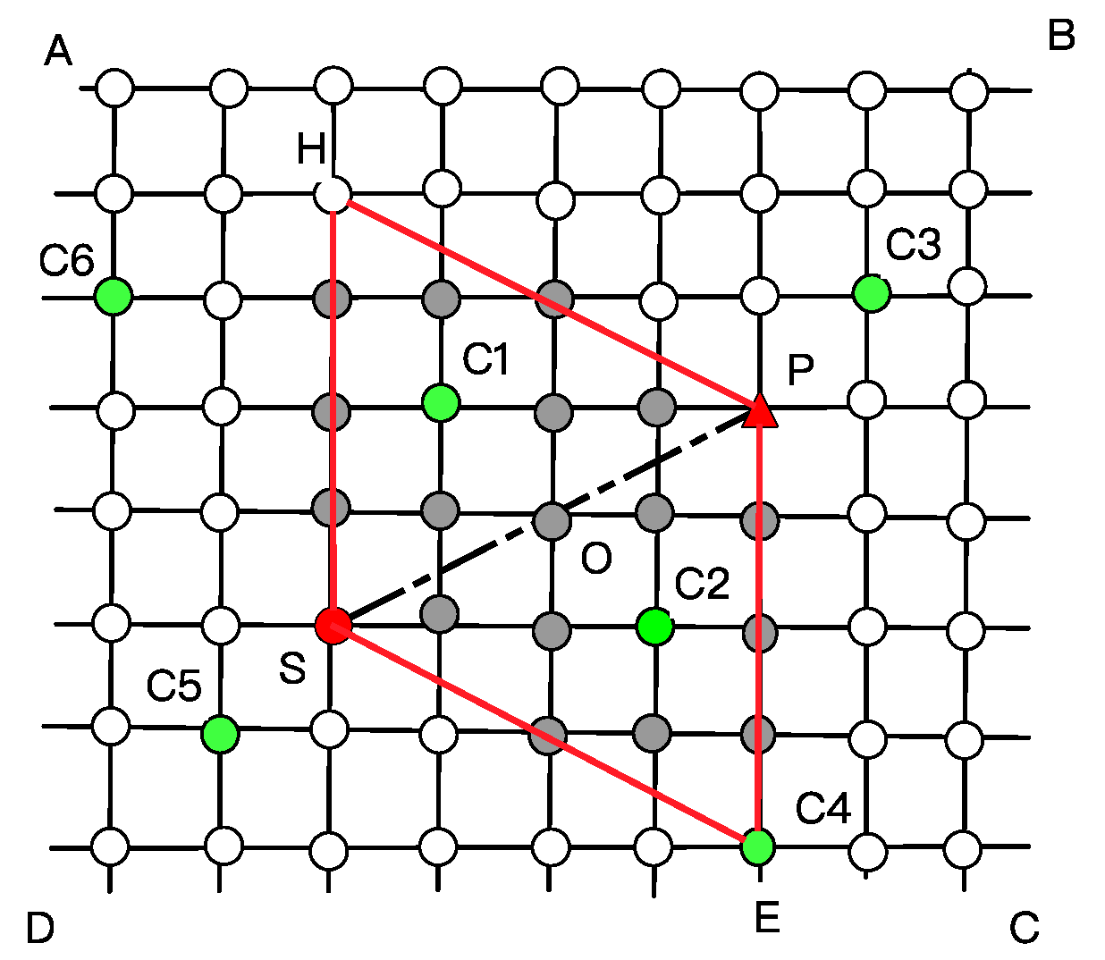
• The line segments of SP and HE show the symmetry of up-down and the symmetry of left-right, respectively.
• The number of nodes contained in the area is significantly smaller than that in the area ABCD.
• The charging station nodes C1 and C2 in the area match with the direction of the users’ next destination and also meet the users’ travel demand.

2.2. Dynamic-Area Construction

To ensure the effectiveness of the charging station network, the dynamic area contains a sufficient number of charging stations. In this section, the AEA is proposed for the area to realize the dynamic extending. The basic idea of the AEA is to extend the distance L in the opposite direction with the charging request point and the next destination point. Then the AEA uses the extended points as two new center points to re-initialize the restricted area, as shown in Figure 3.

There are three cases where the distance L is extended from the center points S and P to the points $S^{\prime }$ and $P^{\prime }$, respectively:

(1) The line segment SP is parallel to the X-axis. Then distance L is extended along the X-axis to get the extended points $S^{\prime }\left(X_{s^{\prime }},Y_{s^{\prime }}\right),P^{\prime }\left(X_{P^{\prime }},Y_{P^{\prime }}\right)$, as shown in Equations (8) and (9).

$$S^{\prime }\left(X_{s^{\prime }},Y_{s^{\prime }}\right)=\{\begin{array}{c}{X}_{S^{\prime }}=X_S-L\\ Y_{S^{\prime }}=Y_S\end{array}$$

(8)

$$P^{\prime }\left(X_{P^{\prime }},Y_{P^{\prime }}\right)=\{\begin{array}{c}{X}_{P^{\prime }}=X_P+L\\ Y_{P^{\prime }}=Y_P\end{array}$$

(9)

(2) The line segment SP is parallel to the Y-axis. Then distance L is extended along the Y-axis to get the extended points $S^{\prime }\left(X_{s^{\prime }},Y_{s^{\prime }}\right),P^{\prime }\left(X_{P^{\prime }},Y_{P^{\prime }}\right)$, as shown in Equations (10) and (11).

$$S^{\prime }\left(X_{s^{\prime }},Y_{s^{\prime }}\right)=\{\begin{array}{c}{X}_{S^{\prime }}=X_S\\ Y_{S^{\prime }}=Y_S-L\end{array}$$

(10)

$$P^{\prime }\left(X_{P^{\prime }},Y_{P^{\prime }}\right)=\{\begin{array}{c}{X}_{P^{\prime }}=X_P\\ Y_{P^{\prime }}=Y_P+L\end{array}$$

(11)

(3) The line segment SP shows a certain angle between the X-axis and the Y-axis; $S^{\prime }$ is the coordinate point of S after extension. Extension at distance L is achieved by $\mathrm{constructing}\mathsf{\Delta }{S}^{\prime }SA$ and $\mathsf{\Delta }\mathrm{O}SB$, as shown in Figure 3. Observing the triangle $\mathsf{\Delta }\mathrm{O}SB$ can get the relationship between the sides, as shown in Equations (12) and (13).

$$\{\begin{array}{c}\left|S{S}^{\prime }\right|=L\\ \left|SB\right|=|X_O-X_S|\\ \left|OB\right|=\left|Y_O-Y_S\right|\end{array}$$

(12)

$$\left|SO\right|=\sqrt[2]{{\left(X_O-X_S\right)}^2+{\left(Y_O-Y_S\right)}^2}$$

(13)

According to the triangle similarity theorem, it can obtain $\mathsf{\Delta }{S}^{\prime }SA\sim \mathsf{\Delta }\mathrm{O}SB$. The relationship is shown in Equation (14).

$$\frac{\left|S{S}^{\prime }\right|}{\left|SO\right|}=\frac{\left|SA\right|}{\left|OB\right|}=\frac{\left|S^{\prime }A\right|}{\left|SB\right|}$$

(14)

Furthermore, the coordinate of $S^{\prime }$ after the extension is shown in Equation (15).

$$S^{\prime }\left(X_{s^{\prime }},Y_{s^{\prime }}\right)=\{\begin{array}{c}{X}_{S^{\prime }}=X_S-\frac{L\times |X_O-X_S|}{\sqrt[2]{{\left(X_O-X_S\right)}^2+{\left(Y_O-Y_S\right)}^2}}\\ Y_{S^{\prime }}=Y_S-\frac{L\times \left|Y_O-Y_S\right|}{\sqrt[2]{{\left(X_O-X_S\right)}^2+{\left(Y_O-Y_S\right)}^2}}\end{array}$$

(15)

In the same way, the coordinate of $P^{\prime }$ after the extension is shown in Equation (16).

$$P^{\prime }\left(X_{P^{\prime }},Y_{P^{\prime }}\right)=\{\begin{array}{c}{X}_{P^{\prime }}=X_P+\frac{L\times \left|X_O-X_P\right|}{\sqrt[2]{{\left(X_O-X_P\right)}^2+{\left(Y_O-Y_P\right)}^2}}\\ Y_{P^{\prime }}=Y_P+\frac{L\times \left|Y_O-Y_S\right|}{\sqrt[2]{{\left(X_O-X_P\right)}^2+{\left(Y_O-Y_P\right)}^2}}\end{array}$$

(16)

Through the discussion of three different cases, the initialized restricted area can be extended dynamically to establish the dynamic-area model according to the users’ travel demand. The dynamic area can continuously extend the range of the area to ensure the effectiveness of the charging station network, and to some extent, limit the number of nodes that needs to traverse in the area. The restricted area initialization and the AEA improve the scalability and robustness of the dynamic-area model.

3. Intelligent Charging Guidance Strategy

The problem of EV charging guidance is essentially a path planning problem from the EV to the charging station. Different from traditional vehicle path planning, intelligent charging guidance needs to ensure that EVs are guided to the charging station in matching their way to destination [12]. How to plan an optimal path for users to match the travel demand and meet charging demand is the research target of the intelligent charging guidance strategy proposed in this section. According to Section 2, a charging station network area that meets the users’ travel demand is constructed based on the dynamic area. However, the number of charging stations in the area is uncertain. Therefore, this section proposes a CAA based on the dynamic area to ensure that the number of charging stations is sufficient. In addition, the shortest-path solution is divided into the charging request point to the charging station (R-C) and the charging station to the next destination(C-N) to find the better travel trips with less travel distance.

3.1. CAA Description

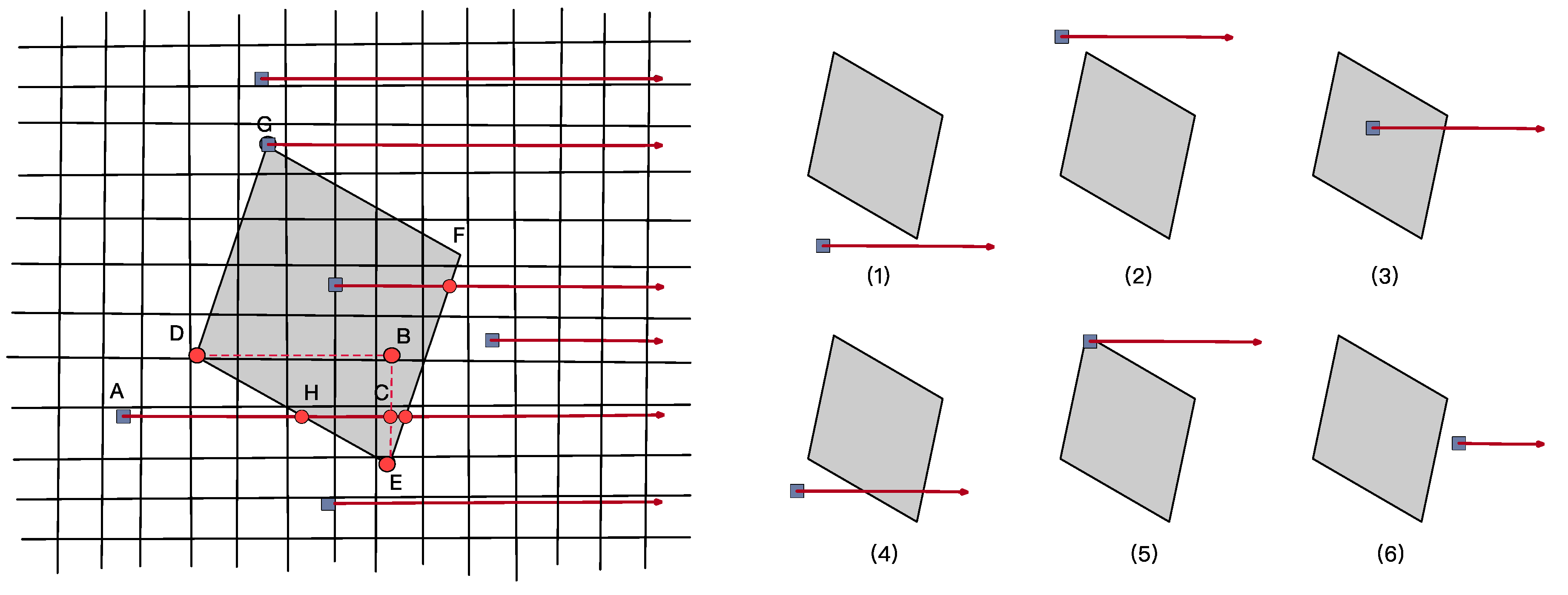
Based on the dynamic area, this paper uses the ray-casting algorithm [28] to detect whether there is a sufficient number of charging stations in the area. The ray-casting algorithm is an algorithm often used to process spatial data. Its basic principle is that the judgment point extends a ray, then calculates the number of intersections between the ray and the boundary of the polygon area according to the number of intersections, determining whether the judgment point is within the area. Because of the symmetry and continuity characteristics of the dynamic area, a CAA is proposed by improving the ray-casting algorithm. The CAA uses the charging station as a judgment point to extend a ray in a specific direction. The point is inside the area if the number of intersections is odd, otherwise, it is outside. As shown in Figure 4, the dynamic area is a prismatic formed by line segments among G, D, F, and E. The square node is assumed as the judgment point. There are six relationships between nodes and the dynamic area by extending the ray indefinitely in the same direction.

The relationships of rays, points, and the dynamic area are summarized into six cases.

(1)

The rays and the points are below the area;

(2)

The rays and the points are above the area;

(3)

Both the rays and the points are in the area;

(4)

The rays pass through the area and the points to the left of the area;

(5)

The rays are outside the area, and the points are at the area boundary;

(6)

The rays and the points are to the right of the area.

According to the relationships, the steps of the CAA are as follows:

(1) Exclude cases where there are no intersections that are cases (1), (2), (6). By judging the coordinate relationship between the charging station and the boundary points G, E, F, it can directly conclude whether the points intersect with the area.

(2) Calculate the number of intersections by constructing similar right triangles. In Figure 4, point A is taken as an example for illustration. By constructing similar right triangles, ΔEBD and ΔECH, the coordinates of points C and B can be obtained based on the given coordinates of points GDEF at the boundary and the judgment point A, as shown in Equations (17) and (18).

$$C(X_C,Y_C)=\{\begin{array}{c}{X}_C=X_E\\ Y_C=Y_A\end{array}$$

(17)

$$B(X_B,Y_B)=\{\begin{array}{c}{X}_B=X_E\\ Y_B=Y_D\end{array}$$

(18)

The linear function $f_{ED}$(x) of the line segment ED is defined by using the two-point formula, as shown in Equation (19).

$$\frac{X-X_E}{X_D-X_E}=\frac{Y-Y_E}{Y_D-Y_E}$$

(19)

Then the coordinate of point H can be obtained, as shown in Equation (20).

$$H(X_H,Y_H)=\{\begin{array}{c}{X}_H=\frac{\left(Y_A-Y_E\right)\times \left(X_D-X_E\right)}{Y_D-Y_E}+X_E\\ Y_H=Y_A\end{array}$$

(20)

Due to ΔEBD~ΔECH, the intersection interval variable τ is calculated by Equation (21).

$$\tau =\left[X_C-\left(Y_E-Y_C\right)\times \frac{X_D-X_B}{Y_E-Y_B}\right]-X_A$$

(21)

where Equation (21) represents the distance from the intersection H to A. When τ > 0, it means that the intersection H is to the right of the ray starting point, and there is one intersection. When τ < 0, it means that the intersection is to the left of the ray starting point A, and there is no intersection.

(3) By traversing the line segments DE and FE with point A, the number of intersections is calculated to determine whether it belongs to the dynamic area.

3.2. Dijkstra for Improving Node Searching Area

The traditional Dijkstra algorithm mainly considers the characteristics of network topology but ignores the structural characteristics of network topology [29]. In general, the time complexity of the Dijkstra algorithm depends on the structural characteristics of the network topology for node searching. When the network topology graph contains a large number of irrelevant nodes, the operation efficiency of Dijkstra will be significantly reduced. To improve the efficiency of node traversal of the Dijkstra algorithm, the earliest proposed algorithm on the structural characteristics of the network topology is Stig [30]. It limits the searching area with nodes through a restricted area. Different from Stig [30], an improved Dijkstra algorithm based on the dynamic area is proposed by improving the scalability of the restricted area.

This paper gives the road network topology graph G, and G is a weighted undirected graph. Let the initial dynamic area be D = ($\alpha ,\beta$) with M nodes, including m charging station nodes, and the final dynamic area $D^{\prime }$ = (${\alpha }^{\prime },{\beta }^{\prime }$) with M’ nodes, including m’ charging station nodes. Where $\alpha$, ${\alpha }^{\prime }$ are the sets of nodes, and $\beta ,{\beta }^{\prime }$ are the sets of edges’ weights. First of all, the initial dynamic area is D constructed from the road network topology graph G, and the list of charging stations in area D is $C_{sta}$. Then, the CAA is used to scan the charging stations in the area and determine whether the number of charging stations n is sufficient to meet $n\ge N$. N is the minimum value of a given charging station, and it can be solved according to the density of charging stations in different areas [31]. If $n\le N$, the AEA is executed by using dynamic distance L to construct a new dynamic area until the number n of charging stations detected by the CAA meets $n\ge N$. Finally, the final dynamic area $D^{\prime }$ can be obtained, and its corresponding list of charging stations is $C_{end}$.

In area D, the node list of the charging station is $C_{sta}$. In area $D^{\prime }$, the node list of the charging station is $C_{end}$. $C_{sta}$ and $C_{end}$ are shown in Equation (22).

$$\{\begin{array}{c}{C}_{sta}=\left[c_1,c_2,c_3,\dots ,c_{\sigma },\dots ,c_m\right],C_{sta}\left[\sigma \right]=c_{\sigma }and\sigma \in \left[1,m\right],G=D\\ C_{end}=\left[c_i,c_j,c_k,\dots ,c_{m^{\prime }}\right],C_{end}\left[k\right]=c_{k}andk\in \left[1,\sigma \right],G=D^{\prime }\end{array}$$

(22)

$C_{sta}$ contains m charging stations before the CAA execution, and each charging station represented by a unique node $c_{\sigma }$. The length of the $C_{end}$ is equal to m’, and m’ ≤ m. It means that there is m’ charging stations after executing the AEA, and each charging station is represented by a unique node $c_k$. The dynamic distance L is calculated according to the number N’ of charging stations in the road network area G and the distance R between the two centers, as shown in Equation (23).

$$L=\frac{R}{N^{\prime }}$$

(23)

Based on the two algorithms AEA and CAA, the improvement process of the node searching area is implemented. The searching area of nodes from area G to area $D^{\prime }$ is significantly reduced by using the adjacency list to store the information of road nodes and charging station nodes. The adjacency list is shown in Figure 5.

After initializing the dynamic area D from G, if the CAA detects the number of charging stations and $C_{sta}$ meets $n\ge N$, then $C_{sta}=C_{end}$, which means the AEA does not need to be executed, and D $=D^{\prime }$. In this case, the time and memory spent on node searching reach the minimum. Otherwise, the AEA is executed multiple times until the dynamic area is large enough for the CAA to detect the number of charging stations. Although the searching area of the nodes after the multiple executions of the AEA will be larger than that without execution, it is still lower than the case of G.

The range of the dynamic area is determined to minimize the total cost of travel, which needs to calculate the minimum total distance from the charging request point to the next destination. Based on Dijkstra to solve the shortest path in the dynamic area, the process of the dynamic area shortest-path algorithm can be divided into three steps. The charging request point defined as $r_i$, the next destination point is $t_i$, and the charging station in the area is $c_{\sigma }$. The three steps are shown below.

-

Step 1: R-C (Request point to Charging station). R-C indicates the shortest-path guidance from the charging request point to the charging station. The shortest-path distance is $l_{RC}$ = $l\left(R_i,C_{\sigma }\right)$, and its corresponding node set is $d_{RC}=d\left(R_i,C_{\sigma }\right)$.

-

Step 2: C-N (Charging station to Next destination). C-N indicates the shortest-path guidance from the charging station to the next destination. The shortest-path distance is $l_{CN}=l\left(C_{\sigma },N_i\right)$, and its corresponding node set is $d_{CN}=d\left(C_{\sigma },N_i\right)$.

-

Step 3: R-N (Request point to Next destination). R-N indicates the process of the dynamic-area shortest-path algorithm from the charging request point to the next destination.

Where $l_{xy}\left(x_i,y_j\right)$ is the representation of the shortest path between nodes. It indicates the shortest-path length from nodes $x_i$ to $y_j$, and the corresponding set of shortest-path nodes is $d_{xy}\left(x_i,y_j\right)$.

Multiple shortest paths and node sets from R-N can be obtained by traversing the list $C_{end}$ of the charging station in the effective dynamic area, as shown in Equation (24).

$$\{\begin{array}{c}{l}_{RN}^i=l_{RC}+l_{CN}\\ d_{RN}^i=d_{RC}{\displaystyle \cup }{d}_{CN}\end{array}andi\in \left[1,n\right]$$

(24)

where $l_{RN}^i$ represents the total travel distance of the i-th user in the R-N, and $d_{RN}^i$ represents the corresponding set of road nodes. By comparing different $l_{RN}^i$ and sorting the distance, it can conclude the shortest-path charging guide plan $\eta$ of the dynamic area, as shown in Equation (25).

$${\eta }_i=\left[\left(l_{RN}^1,d_{RN}^1\right),\left(l_{RN}^2,d_{RN}^2\right),\dots ,\left(l_{RN}^i,d_{RN}^i\right),\dots ,\left(l_{RN}^n,d_{RN}^n\right)\right]andi\in \left[1,n\right]$$

(25)

where n is the number of charging stations in the dynamic area. The charging guidance strategy for the shortest path is ${\eta }_{min}$:

$${\eta }_{min}=min\left({\eta }_i\right)$$

(26)

where ${\eta }_{min}$ is the best charging station planning result in the dynamic area. It meets the shortest total mileage of the travel, and the guided results meet the travel demand and charging demand of users.

3.3. Strategy Structure

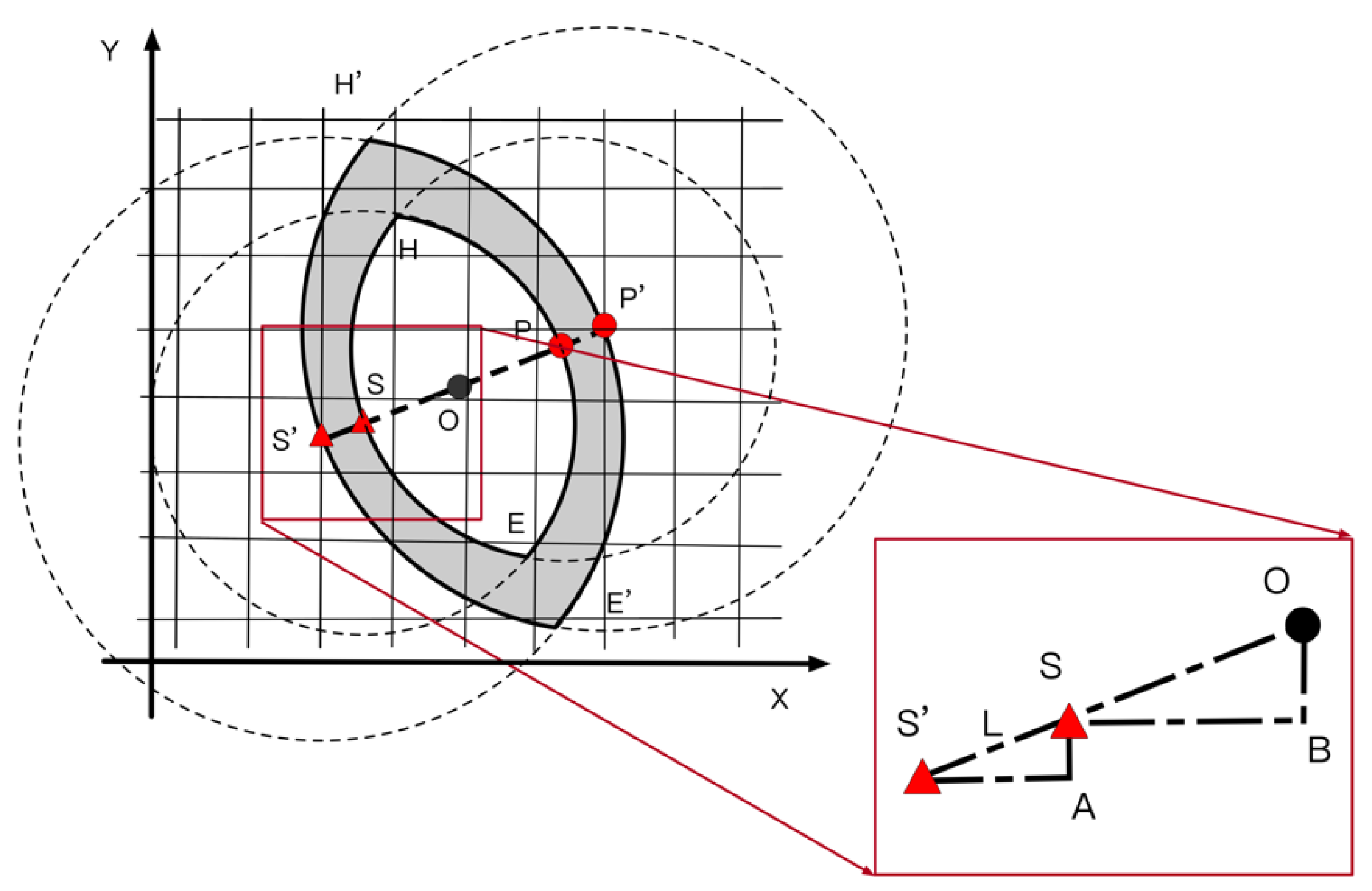
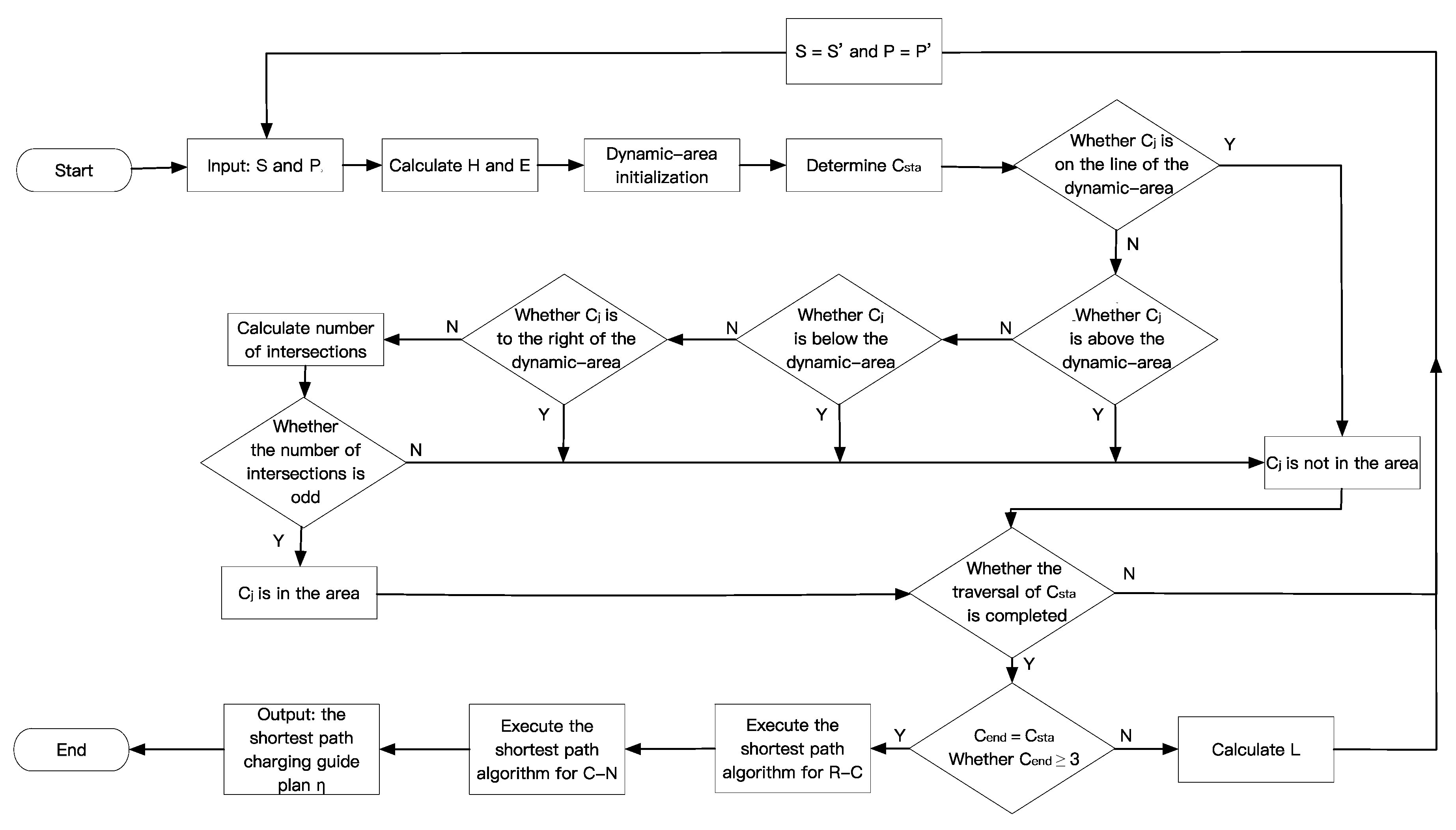
According to Section 3.2, the input and output of the intelligent charging guidance strategy are concluded as follows:

Input: The weighted undirected graph G. It represents road network information. The users’ charging event $U_i=\left(r_i,t_i\right)$ represents the i-th charging request point $r_i$ and next destination initiated $t_i$ obtained by users.

Output: Charging guidance strategy $\eta$, as shown in Equation (25). The charging guidance strategy for the shortest path is ${\eta }_{min}$, as shown in Equation (26).

The execution process of the intelligent charging guidance strategy is shown in Figure 6.

-

Step 1: Determine $U_i=\left(r_i,t_i\right)$ and set $r_i=S$; $t_i=P$, HE points were calculated by Equations (6) and (7). The dynamic area model was established with points HPES.

-

Step 2: Determine the list $C_{sta}$ of charging stations in the area. According to the CAA, traverse the charging stations to determine whether they are within the dynamic area.

-

Step 3: Determine the list $C_{end}$ of charging stations in the dynamic area; the list length is n. Set the sufficient number of charging stations in the dynamic area as 3. If $n\le 3$, execute the AEA and return Step 2; otherwise, execute Step 4.

-

Step 4: Calculate the R-C and C-N distance of each station in the dynamic area. Then, get the R-N calculation results and the list of charging station guidance strategies.

-

Step 5: Calculate the shortest-path charging station guidance strategy ${\eta }_{min}$.

Where, the CAA is executed when the number of charging stations $n$ in the dynamic area is detected each time. Then, the AEA is executed when $n$ in the area does not meet the sufficient number 3. The implementation of the CAA and AEA ensures the dynamic scalability of the dynamic area and the effectiveness of $n$ in the area.

4. Simulation and Results

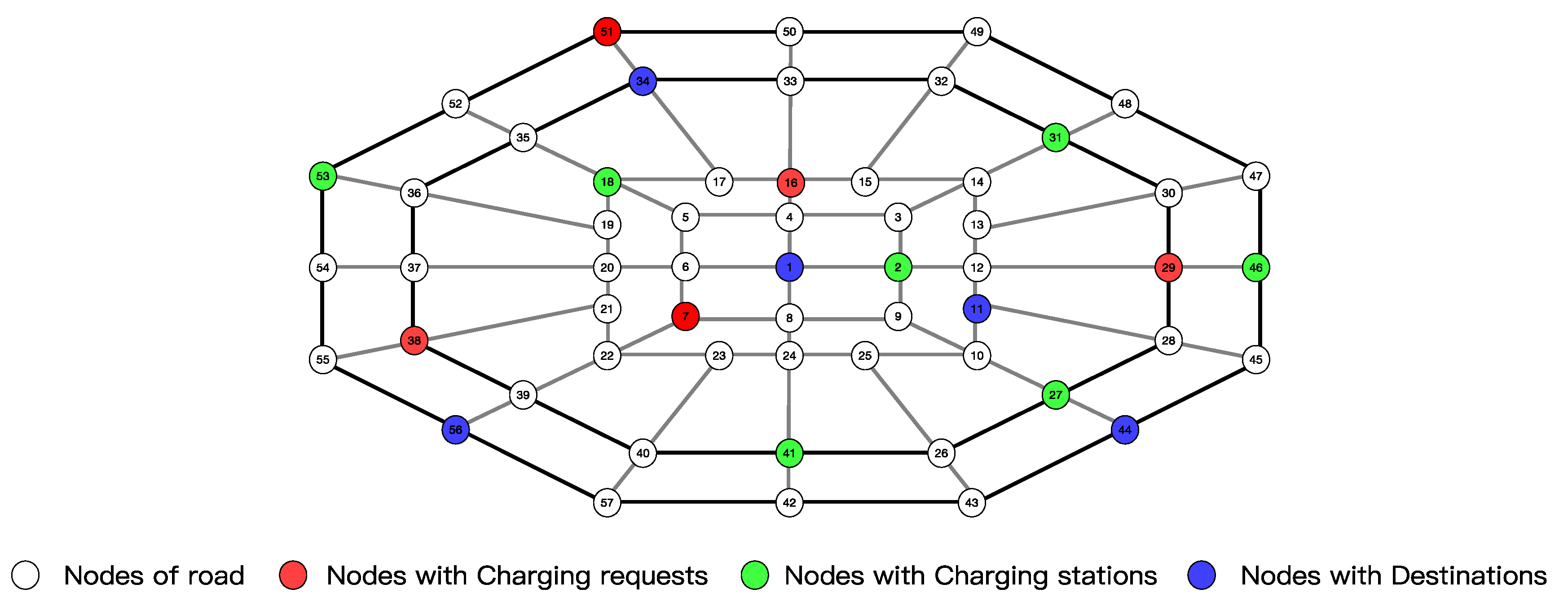
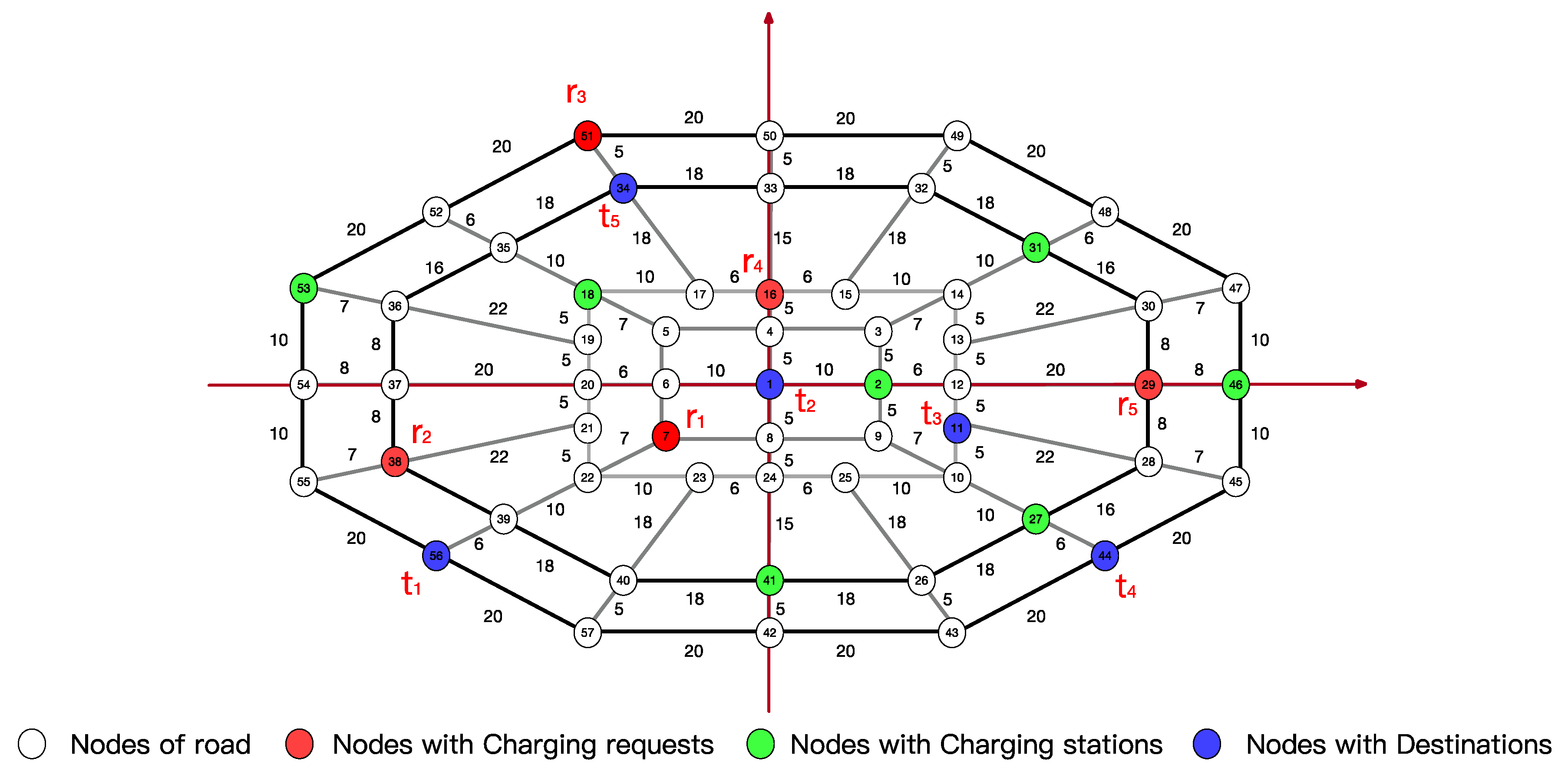
4.1. Road Network Model

In the research of urban road structure, the distance between two points can be expressed by linear distance [32]. Most of the existing research on urban path guidance and planning is based on the urban traffic network graph [1,33]. The usability and extensibility of the urban traffic network graph are of considerable significance to study the effectiveness of algorithms. This paper proposes a hybrid structure of rings and squares to build a road grid model. A square grid is constructed in the central area to emit the radiation path, and the polygon forms a circular and radial mixed road traffic-network structure around the radiation path. As shown in Figure 7, the road network model based on this hybrid structure can serve different urban forms, and the concept of the hybrid structure has also been applied in multiple studies [26,34].

The circular radial traffic network graph in Figure 7 takes the square as the central area and forms the peripheral area in the ring. The line segments between the nodes are straight-line distances, which indicate the two-way road. The effectiveness and applicability of the proposed charging guidance model can be better verified by meshing the urban roads and charging stations.

4.2. Results and Discussion

Based on Figure 7, a coordinate system is established to assign coordinate values to each node in the graph and assign weight values to each link, as shown in Figure 8. The figure contains 57 nodes, including seven charging station nodes, five charging request points $r_1~r_5$, corresponding to five destination nodes $t_1~t_5$, and the rest are ordinary nodes. The length of the line segment between the nodes represents the distance, and the unit is KM.

As shown in Figure 8, the simulation examples of five charging requests to the next destinations are $U_1~U_5$, where U contains the coordinates of the charging request point $r_i\left(x_i,y_i\right)$ and the next destination point $t_i\left(x_i,y_i\right)$. $U_i=\left(r_i,t_i\right)$, indicating the user i initiates the charging request at $r_i$ and gives the next destination $t_i$. The specific data is shown in

Table 1. List of simulation examples.

${\mathit{U}}_{\mathit{i}}\left({\mathit{r}}_{\mathit{i}},{\mathit{t}}_{\mathit{i}}\right)$	${\mathit{U}}_1$	${\mathit{U}}_2$	${\mathit{U}}_3$	${\mathit{U}}_4$	${\mathit{U}}_5$
$r_i$	$r_1=7$	$r_2=38$	$r_3=51$	$r_4=16$	$r_5=29$
$t_i$	$t_1=56$	$t_2=1$	$t_3=11$	$t_4=44$	$t_5=34$
$r_i\left(x_i,y_i\right)$	(−10, −5)	(−36, −8)	(−20, 30)	(0, 10)	(36, 0)
$t_i\left(x_i,y_i\right)$	(−31, −20)	(0, 0)	(16, −5)	(31, −20)	(−18, 25)

.

The simulation data includes the list of charging station nodes $C_{sta}$ and $C_{sta}=\left[c_1,c_2,c_3,c_3,c_5,c_6,c_7\right]$, and the corresponding data are as shown in

Table 2. List of charging stations.

${\mathit{C}}_{\mathit{s}\mathit{t}\mathit{a}}$	Charging Station Node List	Charging Station Coordinates
$c_1$	2	(10, 0)
$c_2$	18	(−16, 10)
$c_3$	27	(26, −15)
$c_4$	31	(26, 15)
$c_5$	41	(0, −25)
$c_6$	46	(44, 0)
$c_7$	53	(−44, 10)

.

According to the intelligent charging guidance strategy proposed in Section 3.3, the model is solved at the charging request point and the next destination given by the simulation example. Based on the simulation data in Table 1, the initial dynamic area D is established, and the minimum number of charging stations in the area is set as $N_{\min }=3$. The results of the final dynamic area $D^{\prime }$ of the users $U_1$ to $U_5$ and the charging strategy ${\eta }^1$ to ${\eta }^5$ can be calculated. They are shown in

Table 3. Results of the intelligent charging guidance strategy. CAA: charging station attribution algorithm.

${\mathit{U}}_{\mathit{i}}\left({\mathit{r}}_{\mathit{i}},{\mathit{t}}_{\mathit{i}}\right)$	$\mathit{D}{\prime }_{\mathit{i}}$	$\left({\mathit{H}}_{\mathit{k}},{\mathit{E}}_{\mathit{k}},{\mathit{S}}_{\mathit{k}},{\mathit{P}}_{\mathit{k}}\right)$	CAA	R	AEA
$U_1\left(7,56\right)$	$D{\prime }_1$	$H_1$(7.11, −51.15)	n = 3 $C=\left[18,53,41\right]$	54.84	Execute 3 times L = 7.83
		$E_1$(−48.11, 26.15)
		$S_1$(1.81, 3.44)
		$P_1$(−42.82, −28.44)
$U_2\left(-36,-8\right)$	$D{\prime }_2$	$H_2$(−47.75, −10.61)	n = 3 $C=\left[18,53,41\right]$	74.58	Execute 1 time L = 10.65
		$E_2$(−6.54, −55.53)
		$S_2$(−29.45, 47.53)
		$P_2$ (11.75, 2.61)
$U_3\left(51,11\right)$	$D{\prime }_3$	$H_3$(7.11, −51.15)	n = 4 $C=\left[2,18,31,53\right]$	64.55	Execute 2 times L = 9.22
		$E_3$(−48.11, 26.15)
		$S_3$ (1.81, 3.44)
		$P_3$(−42.82, −28.44)
$U_4\left(16,44\right)$	$D{\prime }_4$	$H_4$(41.48,21.85)	n = 4 $C=\left[2,27,31,41\right]$	43.14	No execution
		$E_4$(−10.48, −31.85)
		$S_4$ (0, 10)
		$P_4$ (31, −20)
$U_5\left(29,34\right)$	$D{\prime }_5$	$H_5$(30.65, 59.26)	n = 3 $C=\left[2,18,31\right]$	76.51	No execution
		$E_5$(−12.65, −34.26)
		$S_5$ (36, 0)
		$P_5$(−18, 25)

.

Table 3 is the dynamic area established with users $U_1~U_5$. The area meets the travel demand of the users from the charging request points to the next destination points. The four coordinates of the final dynamic area $D^{\prime }$ are $\left(H_{\mathrm{k}},E_{\mathrm{k}},S_{\mathrm{k}},P_{\mathrm{k}}\right)$. Its corresponding number of charging stations n and node list C is detected by the CAA. R is the distance from the charging request point to the next destination point in $D^{\prime }$. The AEA executes different times according to n and L until $n\ge 3$. A schematic diagram of effective dynamic-area calculation results is shown in Figure 9.

In Figure 9, r represents the charging request point, t is the next destination, and c is the charging station. The shaded areas in cases (a) to (e) are the dynamic area, area D is the initial dynamic area, and area $D^{\prime }$ is the final dynamic area. When the number of charging stations in the area does not meet $N_{\min }\ge 3$, the AEA is executed to form the $D^{\prime }$. Cases (a) to (c) show the result of the algorithm execution of $U_1~U_3$, respectively. As the execution frequency increased of the AEA, the range of the dynamic area also extended. In cases (d) and (e), the number of charging stations meets $N_{\min }\ge 3$, thus the AEA is not executed, then $D^{\prime }$ is equal to D. The statistics of the node number in the dynamic area are shown in Figure 10.

Figure 10 shows the number of nodes in the area $D_1^{\prime }~D_5^{\prime }$ after the execution of the AEA. The number of nodes in the initial dynamic area $D_1~D_5$ detected by the CAA is 8, 14, 27, 28, and 22, respectively. Among them, the number of charging stations in the area $D_4~D_5$ already meets the condition $N_{\min }\ge 3$, and only the AEA is performed on $D_1~D_3$. The white part in the figure is the number of newly added nodes in the dynamic extension area, which is 19, 16, and 9, respectively. Compared with the number of nodes in the total area, the number of nodes in $D_1^{\prime }~D_5^{\prime }$ is much smaller due to the improvement of the node searching area based on Dijkstra.

Similar to the charging guidance strategy based on users’ travel destinations, Wang et al. [12] proposed a geometry-based algorithm. Different from the dynamic-area model, Wang et al. [12] selected a charging station for charging by calculating the angle and distance between the charging request point and the destination. The research proposed in this paper does not need to calculate the angle between multiple charging stations and travel planning, and due to the nature of the dynamic-area extension, it has better scalability in the selection of charging stations. However, when the number of charging stations in the initial dynamic area is small and the distribution of the number of charging stations in the area is very sparse, the proposed dynamic-area model will spend more time to calculate the AEA and CAA. Based on the algorithm ideas in [12], this paper uses the simulation examples in Table 1 to calculate the Dijkstra shortest-path algorithm, geometry-based algorithm, and dynamic-area shortest-path algorithm, respectively. Furthermore, Figure 11 presents the results of the algorithms.

As shown in Figure 11, the comparison of the three algorithms on R-C, C-N, and R-N is presented. The case (a) shows the result of different algorithms in R-C. Dijkstra can find the shortest path under different charging requests due to its algorithm characteristics of the shortest path. Because of the limitation of searching direction, the geometric-based algorithm and dynamic-area shortest-path algorithm consume much distance in the process of charging station guidance. The case (b) shows the guidance result of C-N. Both the geometry-based algorithm and the dynamic-area shortest-path algorithm can find the relative shortest path in the process of destination-oriented guidance. Compared with the Dijkstra algorithm, the path guidance with direction achieves specific optimization. At last, the case (c) is R-N, including R-C and C-N. The proposed dynamic-area shortest-path algorithm, because it finds the charging station with the shortest path in the dynamic area, not only meets the users’ travel demand but also always realizes the shortest-path guidance of the total trip. The geometry-based algorithm uses the distance traveled and the angle between the charging station and the destination as the basis for measuring the selection of the charging station. In most cases, it can achieve the shortest guidance for the total trip. However, when there are multiple charging stations with similar distances and angles within the included angle range, the shortest-path charging station is not selected.

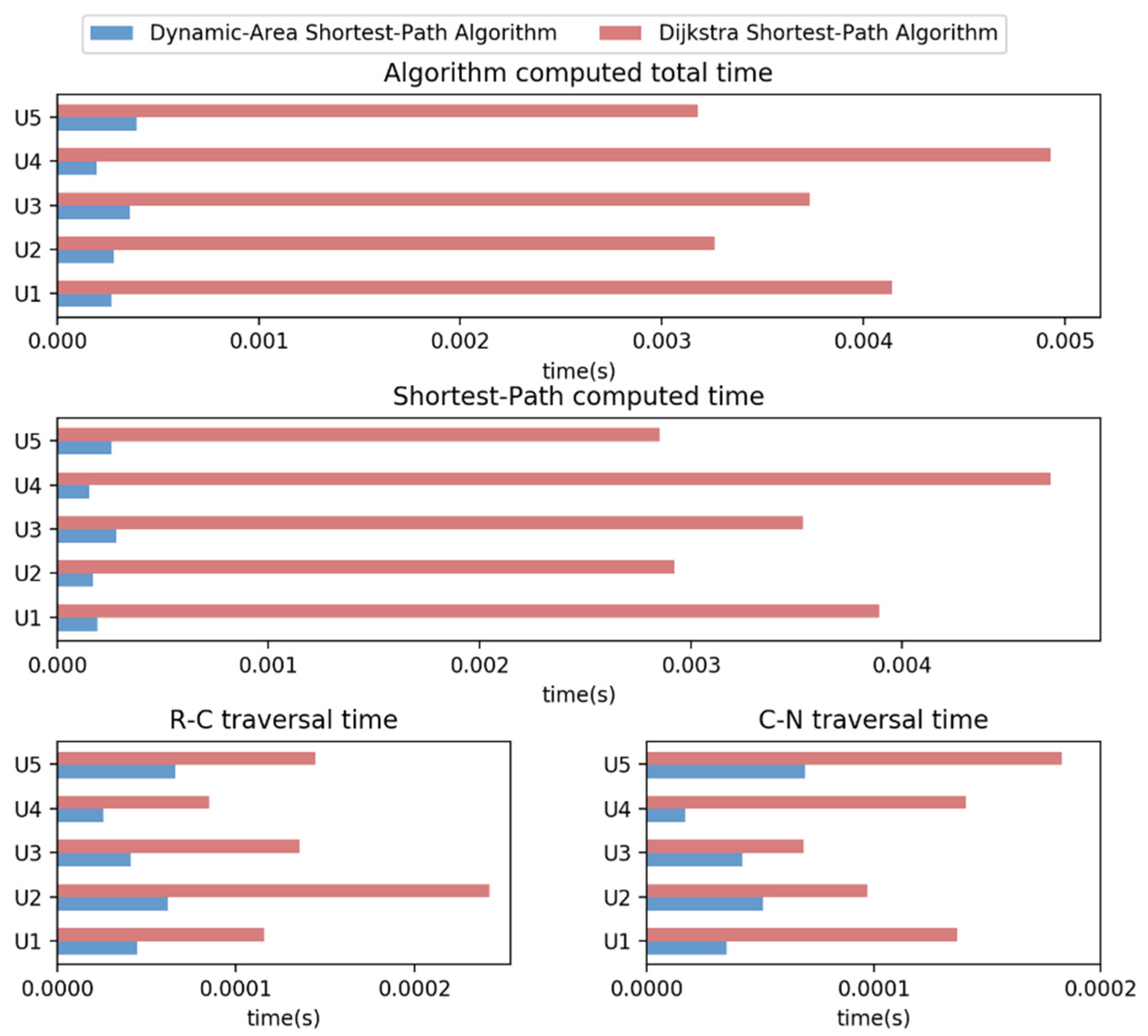
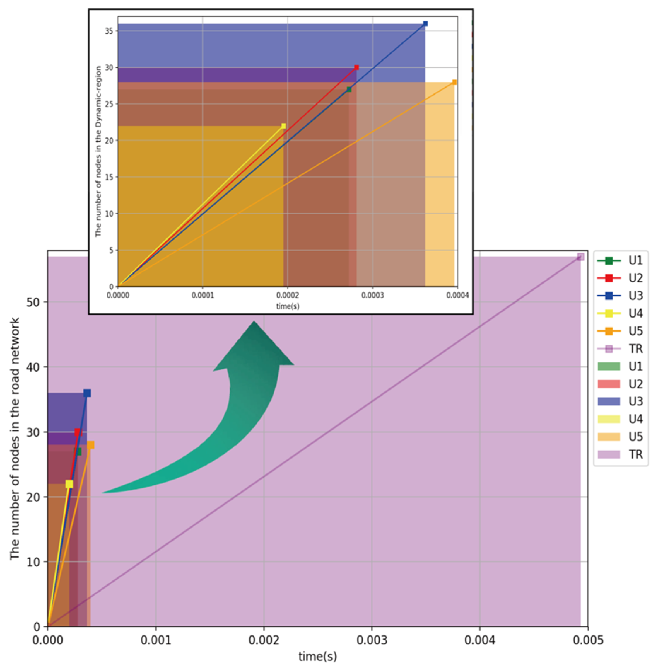
4.3. Comparison of Execution Time

Based on the improved shortest-path algorithm of the restricted area [30], this paper establishes a dynamic area to guide the shortest path and generalizes the reference [30]. To verify the generalization of the dynamic-area shortest-path algorithm, Section 4.3 compared the time performance of the dynamic-area shortest-path algorithm and the traditional Dijkstra algorithm.

This experiment was performed in the same configuration computer (processor 2.6 GHz quad-core Intel Core i7, Memory 16 GB 2133 MHz LPDDR3). Figure 12 shows the execution results of computed time and traversal time.

In Figure 12, the comparison results of the shortest-path computed time and node traversal time are shown respectively. Due to the limited nodes of the simulated road network model, the computing time of the computer is very low. However, we know that the Dijkstra algorithm is realized by traversing all nodes in the graph. Therefore, under the condition that the starting point and ending point of charging events remain unchanged, increasing nodes of the simulation road network model will not increase the time complexity of the proposed model, but will increase the time complexity of the traditional algorithm. By comparing with the computed total time between the two algorithms, the computed time reaches a minimum of 0.0001950 s on the dynamic-area shortest-path algorithm, but the corresponding Dijkstra algorithm reaches a maximum of 0.00493 s. It is indicated that the dynamic-area shortest-path algorithm can effectively reduce the number of nodes and computed time in the node traversal and calculation. Similarly, in the calculation of charging requests from $U_1$ to $U_5$, the computed time of the dynamic-area shortest-path algorithm is far less than that of the Dijkstra algorithm. By reducing invalid nodes, the dynamic-area shortest-path algorithm effectively reduces the time consumed in node traversal. The node traversal time of the R-C and the C-N shows that the dynamic-area shortest-path algorithm keeps the minimum time, unlike the Dijkstra algorithm.

In charging events $U_1~U_5$, the dynamic-area shortest-path algorithm shows the traversal time of nodes significantly reduced by comparing with the Dijkstra algorithm, and the dynamic-area shortest-path computed time is 91.74% lower on average. Figure 13 shows the comparison of the node traversal time between the Dijkstra algorithm and the dynamic-area shortest-path algorithm.

Figure 13 shows the relationship between the algorithm average computation time and the number of nodes in the road network. In Figure 13, TR represents the total road network with all nodes. From the shaded area in the figure, it can intuitively obtain the time to node comparison effect of the charging events $U_1~U_5$ and TR. The size of the shaded area can intuitively show the time consumed by the algorithm execution. In addition, the diagonal slope in the shaded area is the density K, and the unit is number/ms. As the number of nodes traversed increases, the time consumption becomes higher, and the density K becomes smaller. The K of each charging event is shown in

Table 4. Density value K.

	${\mathit{U}}_1$	${\mathit{U}}_2$	${\mathit{U}}_3$	${\mathit{U}}_4$	${\mathit{U}}_5$	TR
K	99.26	106.83	99.47	112.82	70.70	11.56

.

The more considerable density value indicates that more nodes can be traversed in a certain period. In the $U_1~U_5$ area, the density value is higher than that of TR. When traversing all the nodes in the TR area, the density reaches the minimum. The K in Table 4 shows the dynamic area can always keep the value higher than Dijkstra, which means the AEA and CAA proposed in this paper are effective.

5. Conclusions

As the number of EVs continues to increase, guiding EV users effectively to charging stations is of considerable significance for alleviating users’ charging anxiety. This paper proposed an intelligent charging strategy to study the travel demand and charging demand of EV users. In the study of users’ travel demand, the Dijkstra algorithm is improved based on the dynamic-area model. By improving the searching area of nodes, the direction of the charging guidance is set intelligently to find the charging stations consistent with users’ destinations. In the study of charging demand, the charging strategy realized in the dynamic area for users to find the shortest travel path. The CAA and AEA are designed to improve the robustness and reliability of the intelligent charging guidance strategy. Both of the two algorithms are based on the dynamic-area model to ensure a sufficient number of charging stations. The main contribution of the intelligent charging guidance strategy is concluded to be that it makes EV charging guidance more in line with users’ travel demand and charging demand. Furthermore, it improves the operating efficiency of the Dijkstra algorithm and the timeliness of the guidance algorithm. In the real world, maps are calculated by latitude and longitude. Therefore, the input data of the proposed model can be well replaced by latitude and longitude and applied to the navigation of the real world.

In this study, factors such as the remaining driving range of EVs and road congestion were not taken into account. The proposed model cannot calculate whether the charging station is within the reachable range based on the remaining mileage of the EV but matches charging stations for the EV based on the dynamic area. Further research will consider a given initial SOC (State of Charge) value and add the road congestion covered in the dynamic area.

References

1. Lin, Z.-P.; Wang, H.-S.; Tsai, S.-J. The Intelligent Charging Path Planning for Electric Vehicle. Int. J. Comput. Netw. Wirel. Mob. Commun. (IJCNWMC) 2016, 6, 1–8. [Google Scholar]
2. Bonges, H.A.; Lusk, A. Addressing electric vehicle (EV) sales and range anxiety through parking layout, policy and regulation. Transp. Res. Part. A Policy Pract. 2016, 83, 63–73. [Google Scholar] [CrossRef] [Green Version]
3. Guo, F.; Yang, J.; Lu, J. The battery charging station location problem: Impact of users’ range anxiety and distance convenience. Transp. Res. Part. E Logist. Transp. Rev. 2018, 114, 1–18. [Google Scholar] [CrossRef]
4. Li, S.; Tong, L.; Xing, J.; Zhou, Y. The Market for Electric Vehicles: Indirect Network Effects and Policy Design. J. Assoc. Environ. Resour. Econ. 2017, 4, 89–133. [Google Scholar] [CrossRef]
5. Dong, J.; Xie, M.; Zhao, L.; Shang, D. A framework for electric vehicle charging-point network optimization. IBM J. Res. Dev. 2013, 57, 15:1–15:9. [Google Scholar] [CrossRef]
6. Gong, L.; Cao, W.; Liu, K.; Zhao, J.; Li, X. Spatial and Temporal Optimization Strategy for Plug-In Electric Vehicle Charging to Mitigate Impacts on Distribution Network. Energies 2018, 11, 1373. [Google Scholar] [CrossRef] [Green Version]
7. Suyono, H.; Rahman, M.T.; Mokhlis, H.; Othman, M.; Illias, H.A.; Mohamad, H. Optimal Scheduling of Plug-in Electric Vehicle Charging Including Time-of-Use Tariff to Minimize Cost and System Stress. Energies 2019, 12, 1500. [Google Scholar] [CrossRef] [Green Version]
8. Kongjeen, Y.; Bhumkittipich, K. Impact of Plug-in Electric Vehicles Integrated into Power Distribution System Based on Voltage-Dependent Power Flow Analysis. Energies 2018, 11, 1571. [Google Scholar] [CrossRef] [Green Version]
9. Gao, Y.; Guo, S.; Ren, J.; Zhao, Z.; Ehsan, A.; Zheng, Y. An Electric Bus Power Consumption Model and Optimization of Charging Scheduling Concerning Multi-External Factors. Energies 2018, 11, 2060. [Google Scholar] [CrossRef] [Green Version]
10. Mao, T.; Zhang, X.; Zhou, B. Intelligent Energy Management Algorithms for EV-charging Scheduling with Consideration of Multiple EV Charging Modes. Energies 2019, 12, 265. [Google Scholar] [CrossRef] [Green Version]
11. Lopez, K.L.; Gagne, C.; Gardner, M.-A. Demand-Side Management Using Deep Learning for Smart Charging of Electric Vehicles. IEEE Trans. Smart Grid 2018, 10, 2683–2691. [Google Scholar] [CrossRef]
12. Wang, Y.; Bi, J.; Zhao, X.; Guan, W. A geometry-based algorithm to provide guidance for electric vehicle charging. Transp. Res. Part. D Transp. Environ. 2018, 63, 890–906. [Google Scholar] [CrossRef]
13. Baum, M.; Dibbelt, J.; Gemsa, A.; Wagner, D.; Zündorf, T. Shortest Feasible Paths with Charging Stops for Battery Electric Vehicles. In Proceedings of the 23rd SIGSPATIAL International Conference on Advances in Geographic Information Systems-GIS’ 15, Seattle, WA, USA, 3–6 November 2015; pp. 1–10. [Google Scholar]
14. Chunping, Y.; Qi, Z.; Bing, Q.; Bin, L.; Gaoying, C. Charge and discharge scheduling strategy of electric vehicle based on interest and travel intention of users. Electr. Meas. Instrum. 2018, 684, 112–118. [Google Scholar]
15. Schwenk, K.; Faix, M.; Mikut, R.; Hagenmeyer, V.; Appino, R.R. On Calendar-Based Scheduling for User-Friendly Charging of Plug-In Electric Vehicles. In Proceedings of the 2019 IEEE 2nd Connected and Automated Vehicles Symposium (CAVS), Honolulu, HI, USA, 22–23 September 2019; pp. 1–5. [Google Scholar]
16. De, H.J.; Alpcan, T.; Brazil, M.; Thomas, D.; Mareels, I. A Market Mechanism for Electric Vehicle Charging Under Network Constraints. IEEE Trans. Smart Grid 2015, 7, 827–836. [Google Scholar] [CrossRef]
17. Wang, Y.; Bi, J.; Guan, W.; Zhao, X. Optimising route choices for the travelling and charging of battery electric vehicles by considering multiple objectives. Transp. Res. Part. D Transp. Environ. 2018, 64, 246–261. [Google Scholar] [CrossRef]
18. Fei, W.; Li, Z.; Ye, M. Review on research of impact of electric vehicles charging on power grids and its optimal dispatch. South. Power Syst. Technol. 2016, 10, 71–80. [Google Scholar]
19. Vandael, S.; Claessens, B.; Ernst, D.; Holvoet, T.; Deconinck, G. Reinforcement Learning of Heuristic EV Fleet Charging in a Day-Ahead Electricity Market. IEEE Trans. Smart Grid 2015, 6, 1. [Google Scholar] [CrossRef] [Green Version]
20. Tan, J.; Wang, L. Real-time charging navigation of electric vehicles: A non-cooperative game approach. In Proceedings of the 2015 IEEE Power & Energy Society General Meeting, Denver, CO, USA, 26–30 July 2015; pp. 1–5. [Google Scholar] [CrossRef]
21. Chau, S.C.-K.; Elbassioni, K.; Tseng, C.-M. Drive Mode Optimization and Path Planning for Plug-In Hybrid Electric Vehicles. IEEE Trans. Intell. Transp. Syst. 2017, 18, 3421–3432. [Google Scholar] [CrossRef] [Green Version]
22. Liu, H.; Yin, W.; Yuan, X.; Niu, M. Reserving Charging Decision-Making Model and Route Plan for Electric Vehicles Considering Information of Traffic asnd Charging Station. Sustainability 2018, 10, 1324. [Google Scholar] [CrossRef] [Green Version]
23. Black, A. Optimizing urban mass transit systems: A general model. Transp. Res. Rec. 1976, 610, 12–18. [Google Scholar]
24. Zhang, Y.; Aliya, B.; Zhou, Y.; You, I.; Zhang, X.; Pau, G.; Collotta, M. Shortest feasible paths with partial charging for battery-powered electric vehicles in smart cities. Pervasive Mob. Comput. 2018, 50, 82–93. [Google Scholar] [CrossRef]
25. Wang, Y.; Bi, J.; Lu, C.; Ding, C. Route Guidance Strategies for Electric Vehicles by Considering Stochastic Charging Demands in a Time-Varying Road Network. Energies 2020, 13, 2287. [Google Scholar] [CrossRef]
26. Luo, S.; Nie, Y. (Marco) On the role of route choice modeling in transit sketchy design. Transp. Res. Part. A Policy Pract. 2020, 136, 223–243. [Google Scholar] [CrossRef]
27. Chen, H.; Gu, W.; Cassidy, M.J.; Daganzo, C.F. Optimal transit service atop ring-radial and grid street networks: A continuum approximation design method and comparisons. Transp. Res. Part. B Methodol. 2015, 81, 755–774. [Google Scholar] [CrossRef] [Green Version]
28. Shimrat, M. Algorithm 112: Position of point relative to polygon. Commun. ACM 1962, 5, 434. [Google Scholar] [CrossRef]
29. Wang, H.; Zhou, X. Improved shortest path algorithm for restricted searching area. J. Nanjing Univ. Sci. Technol. (Nat. Sci.) 2009, 5, 638–642. [Google Scholar]
30. Nordbeck, S. Computer cartography, shortest route programs. Lund Stud. Geogr. Ser. C 1969, 9, 53. [Google Scholar]
31. Chu, Y.J.; Ma, L.; Zhang, H.Z. Location-allocation and Its Algorithm for Gradual Covering Electric Vehicle Charging Stations. Math. Pract. Theory 2015, 45, 102–106. [Google Scholar]
32. Badia, H.; Estrada, M.; Robusté, F. Competitive transit network design in cities with radial street patterns. Transp. Res. Part. B Methodol. 2014, 59, 161–181. [Google Scholar] [CrossRef]
33. Miyagawa, M. Optimal hierarchical system of a grid road network. Ann. Oper. Res. 2009, 172, 349–361. [Google Scholar] [CrossRef]
34. Fan, W.; Mei, Y.; Gu, W. Optimal design of intersecting bimodal transit networks in a grid city. Transp. Res. Part. B Methodol. 2018, 111, 203–226. [Google Scholar] [CrossRef]
Figure 1. Network topology graph of the restricted area.
Sustainability 12 07343 g001
Figure 2. Network topology of a prismatic dynamic area.
Sustainability 12 07343 g002
Figure 3. Schematic diagram of the area extension algorithm (AEA).
Sustainability 12 07343 g003
Figure 4. Charging station attribution algorithm.
Sustainability 12 07343 g004
Figure 5. The changing process of the node searching space.
Sustainability 12 07343 g005
Figure 6. Flow chart of the intelligent charging guidance strategy.
Sustainability 12 07343 g006
Figure 7. Road network topology graph.
Sustainability 12 07343 g007
Figure 8. Schematic diagram of a simulation example.
Sustainability 12 07343 g008
Figure 9. Schematic diagram of D and D . (a) U 1 ’s dynamic area change diagram. (b) U 2 ’s dynamic area change diagram. (c) U 3 ’s dynamic area change diagram. (d) U 4 ’s dynamic area change diagram. (e) U 5 ’s dynamic area change diagram.
Sustainability 12 07343 g009
Figure 10. Comparison of the number of nodes in the area.
Sustainability 12 07343 g010
Figure 11. Comparison of distance on (a) R-C, (b) C-N and (c) R-N.
Sustainability 12 07343 g011
Figure 12. Comparison of algorithm consumption time.
Sustainability 12 07343 g012
Figure 13. Node traversal time comparison.
Sustainability 12 07343 g013