Article

The Impact of Urban Form and Spatial Structure on per Capita Carbon Footprint in U.S. Larger Metropolitan Areas

1
Department of Applied Economics, Universidad Autónoma de Barcelona, 08193 Bellaterra, Barcelona, Spain
2
School of Economics, Universidad Sergio Arboleda, 110221 Bogotá, Colombia
*
Author to whom correspondence should be addressed.
Sustainability 2020, 12(1), 389; https://doi.org/10.3390/su12010389
Submission received: 18 October 2019 / Revised: 23 December 2019 / Accepted: 27 December 2019 / Published: 3 January 2020
(This article belongs to the Special Issue Urban Regeneration and Sustainable Urban Development)

Abstract

:
Different studies have estimated cities’ contribution to total greenhouse gas (GHG) emissions at between forty and seventy percent. According to the so-called Compact City Approach, high density and centrality should lead to low GHG. This study compares the effect of the urban density and spatial structure (monocentrism, polycentrism, and dispersion) of the main U.S. cities on their greenhouse gas emissions from mobility and housing. The estimated models include control variables in order to improve the statistical adjustment, these variables are grouped into three categories: basic controls as temperature and Gross Domestic Product (GDP); historical-demographic controls since 1900; and geographic-urban planning controls. The results detect an environmentally positive effect, albeit a moderate one, associated with monocentric and polycentric spatial structures as compared to dispersed structures. Within the tradition of urban planning, these results can be used as an argument to stop the dispersed decentralization of cities. However, the efficacy of some policies encouraging density should be accompanied by specific policies which increase the energy efficiency of housing and promote the use of public transport.

1. Introduction

Different studies have estimated cities’ contribution to total greenhouse gas (GHG) emissions at between forty and seventy percent [1,2,3,4,5]. With more than half of the world’s population living in cities, designing policies to lower greenhouse gas (GHG) emissions on an urban scale seems like a sound strategy in the struggle against climate change. According to the so-called Compact City Approach [6,7,8], dense and centralized cities have lower per capita emissions in comparison with low-density dispersed cities, given that in the former cars are used less and commuting distances are shorter [9,10,11,12,13,14,15], and the buildings require less energy to reach an acceptable climate comfort level [16,17,18]. Continuing along this line of argumentation, urban planning policies modify the built environment (urban form and spatial structure) of cities, which should affect their volume of GHG emissions.
There is an extensive literature on the environmental benefits of compactness (high density and high centrality) associated with low energy consumption in mobility [17,19,20,21,22,23,24,25,26,27,28,29,30] and housing [16,17,18]. In the case of mobility, compactness facilitates travel on foot or by public transport [13,15] and reduces commuting distances [31,32,33,34,35,36]. In the case of housing, the type of residential buildings in dense neighborhoods is characterized by the small size of the houses and the existence of shared walls, which leads to low energy consumption [16,17,18,37].
The Brookings Institution funded an ambitious project to measure the carbon footprint of mobility and housing in the 100 largest urban areas in the United States. By using multivariate Ordinary Least Squares (OLS) regression models, the per capita footprint is explained by built environment indicators (population density, employment density, population concentration index) and other control variables. The methodology used can be consulted in working papers [38,39,40] and in academic journals [41,42]. The main result of the project is that the concentration of population leads to a smaller per capita carbon footprint, which coincides with the predictions that emerge from the Compact City Approach. The problem of using a concentration index as regressor is that it is correlated with the population density and urban spatial structure regressors [43]. In addition, the concentration indicator tells us little about the spatial structure (monocentrism, polycentrism, or dispersion), an aspect that, according to numerous investigations, may help to explain the variability observed in the per capita carbon footprint [44,45,46,47,48,49].
Given these doubts, the research carried out analyzes the impact of urban form (population density) and spatial structure (indicators of monocentrism, polycentrism, and dispersion) of larger U.S. urban areas on their carbon footprint in mobility and housing. For this purpose, the carbon footprint data on mobility and housing calculated in Brown et al. [38] for the year 2000 are used as a dependent variable. In order to compare the extent to which the results are affected by the methodology for calculating the carbon footprint, by the control variables incorporated in the models, or by the econometric method used, we re-estimate the same models, with the same method (OLS), and with the same explanatory variables, but in this case using the carbon footprint data in mobility and housing calculated by the authors of Glaeser and Kahn [44].
Considering the methodology used, the CO2 emissions indicator values that appear in Glaeser and Kahn [44] and Brown et al. [38] can be considered quasi-carbon footprints. As in the case of carbon footprints, the emissions calculated in both investigations are accounted for at the place of consumption. This is important, given that CO2 emissions associated with the consumption of electric energy are charged to the households that use this energy, even if the actual CO2 emissions required to obtain the electric energy have originated outside the metropolitan area. However, unlike carbon footprints, they do not consider indirect emissions embodied in buildings, transport infrastructures, and vehicles. The authors of reference [41] argue that this is the main limitation of their research for the Brookings Institution that can be consulted in several publications [38,39,40,41,42]. The results obtained in these studies are very optimistic regarding the role of Compact City policies as an instrument to reduce the carbon footprint of cities.
The study for the Brookings Institution and Glaeser and Kahn [44] are similar in several aspects, which facilitates their comparison. Both studies offer results for the same group of American cities, the same type of consumption (mobility and housing); the same year (2000); and estimate the same type of multivariate regression models (OLS). The main difference is that the Brookings Institution studies consider average per capita carbon footprint as a dependent variable, while the authors of Glaeser and Kahn [44] consider the marginal emissions corresponding to families living in buildings built between 1980 and 2000. This explains the fact that the volume of per capita emissions calculated by the authors of Glaeser and Kahn [44] is systematically higher than that calculated in the studies for the Brookings Institution.
There are two questions that we intend to answer with this study. The first is whether density effectively exerts a negative sign impact on the carbon footprint of American cities in mobility and housing (higher density implies a lower footprint) considering that the statistical significance of the parameter obtained may be affected by the combination of socio-economic and geographic control variables included as regressors. The second is, what is the effect of spatial structure on the carbon footprint, including the monocentric, the polycentric, and the dispersed as possible spatial structures. This exercise therefore has the virtue of offering a framework with which to compare the studies of the Brookings Institution and the research in Glaeser and Kahn [44]. The impact of polycentrism on mobility is a dynamic novel line of research. Some studies found that living near a sub-center tends to decrease commuting distance [31,32,33,34,35,36]. Therefore, it is reasonable to hypothesize that polycentrism can reduce the carbon footprint. For instance, authors of references [48,49,50] find environmental benefits associated with polycentricity in terms of low carbon footprint.

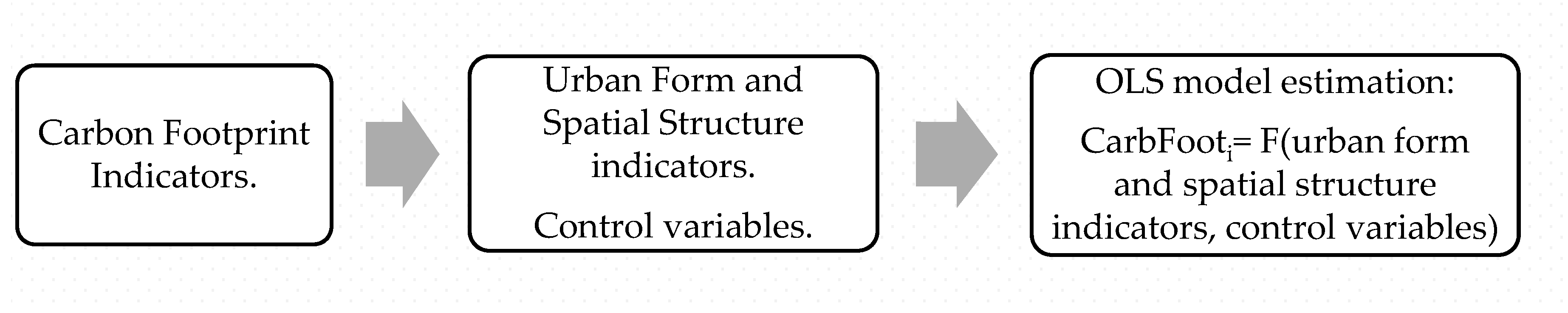
2. Methodology and Data

2.1. Methodology

This section explains the procedure used to capture the relationship between cities’ urban form and spatial structure and their per capita carbon footprint from mobility and housing. As Figure 1 shows, we used multivariate regression models that explain the variability observed in the carbon footprint according to different explanatory variables, including built environment variables. The database used in this study is comprised of the most populous U.S. Metropolitan Areas (between 45 and 58 urban areas depending on the estimated model). The software used to estimate the model is STATA(R).
Different multivariate regression models are estimated through Ordinary Least Squares (OLS), using per capita carbon footprint associated with energy consumption from housing (electricity and fuel), from mobility in private vehicles, and the sum of both as dependent variable. The models were estimated by first incorporating all the control variables, and then adding the built environment variables one by one, given that they are strongly correlated. Then, the control variables with no significant coefficients were removed. This method enabled spurious causality problems to be controlled. Each estimated model includes different combinations of control variables. The results of the models reported in this document were chosen according to the significance of the built environment parameters as well as the model’s overall explanatory capacity (Adjusted R2). In formal terms the regression model is written as follows:
Y j = α + k β k X k + e j
where Y j represents the dependent variable (per capita carbon footprint), α is the constant term, β k represents the estimated coefficient of the explanation variable X k , and e j is the residual term of the regression equation.

2.2. Dataset

2.2.1. Carbon Footprint Indicators

Two studies [38,44] are essential to this research paper, given that we use their per capita carbon footprint as dependent variables in the OLS regression models. There are two main differences between both studies. First, they differ in terms of the unit of measurement (tons vs. pounds), the scale used (household vs. individual), the use of logarithms, and the number of cities considered. (On the other hand, Glaeser and Kahn [44] offers results for the footprint from public transport, while authors of Brown et al. [38] do not. We have standardized emissions in per capita tons of CO2. The data from Glaeser and Kahn [44] were originally presented in pounds per household, so they had to be transformed using the corresponding conversion factors 2.204 lbs/kg; 2.58 persons/household (mean in the USA). This latter indicator was applied countrywide. Each state has minor differences in household size that we have incorporated into the calculation.) Second, Brown et al. [38] calculates the carbon footprint of the average inhabitant, while Glaeser and Kahn [44] takes a standard household with an income of $62,500, 2.62 members, and a head of household aged 49 as the reference. In this way, the authors in Glaeser and Kahn [44] seek to capture the marginal effect of a new household, which is assumed to be higher than the effect of the average household. The correlation between both total footprint indicators is 0.57.
The procedure used by Brown et al. [38] to calculate the carbon footprint of gasoline used by private cars follows these steps: (a) calculate the average distance of journeys with data on the car fleet on American highways; (b) rescale the results until reaching the metropolitan scale, and (c) convert the consumption of fuels into CO2 emissions with the appropriate conversion factors. To calculate the residential-fuel footprint, the following steps are taken: (a) estimate fuel consumption per family for each state, (b) allocate fuel consumption by type of dwelling, (c) assign the number of households to each type of dwelling, (d) allocate fuel consumption at the metropolitan scale according to the different housing categories in each state; (e) estimate fuel consumption at the metropolitan scale, and (f) convert fuel consumption into CO2 emissions. Regarding the residential-electricity calculation carbon footprint: (a) it is based on data on household electricity consumption for each utility, (b) the number of households for each city and for each utility is estimated, (c) the total consumption is estimated at zip code level, (d) the results are added together at the county level; (e) the estimated consumptions included in the rents are added as a fixed income, the results are added together at the metropolitan level, and (f) consumption is converted into CO2 emissions.
The carbon footprint values calculated by the authors in Glaeser and Kahn [44] are obtained from similar, but not totally coincident, procedures. In addition, the databases are different. To estimate the gasoline footprint they: (a) estimate data on miles traveled from a model that includes socio-economic variables of individuals and each zip code, (b) estimate the gasoline consumption of a family with an income of $62,500 and an occupation of 2.62 individuals per household, and (c) add together the data of each zip code until a metropolitan area is conformed. To estimate the residential-fuel carbon footprint: (a) gas consumption is estimated based on individual characteristics for each metropolitan area for an average household, and (b) the consumption of gas and fuel oil is converted into CO2 emissions by applying the conversion factors. To estimate the carbon footprint of electricity, the following steps are followed: (a) household expenditure on electricity is estimated considering individual characteristics of each metropolitan area, (b) consumption expenditure is converted, taking into account regional electricity markets and primary sources, and (c) electricity consumption is converted into CO2 emissions. Table A1 and Table A2 in Appendix A summarize these two methodologies described above.

2.2.2. Explanatory Variables

Urban Form. Population density for 2000: this is the population per square mile from the US Census Bureau (Population Housing Units Area and Density 2000).
Urban Spatial structure. The spatial structure indicators estimated by the authors of reference [51] were used. The authors of reference [51] propose a simple, clear, and replicable methodology for measuring urban spatial structure of large urban areas. The employment centers were previously identified using a methodology based on reference [52] Geographically Weighted Regression in which the Traffic Analysis Zones (TAZs) have an employment density significantly higher than what would be predicted based on their location. The centrality (monocentrism) indicator is the percentage of jobs located in the center (CBD), the polycentrism indicator is the percentage of jobs concentrated in the employment sub-centers, and the sprawl indicator is the percentage of jobs located outside the centers and sub-centers. These spatial structure indicators were first proposed by the authors of reference [53] and applied in numerous studies, including the research in references [36,54,55,56,57,58,59,60]. Two alternative indicators of centrality and polycentrism, very generously provided by reference [61], were also used. The methodology may be consulted in reference [61]. They use spatial econometrics (Moran Index) to identify the subcenters and the indices of monocentrism and polycentrism are calculated using the principal component method applied to various aspects that have to do with mobility and also with the sectoral specialization in certain activities.
The control variables used in the regression models are grouped into three categories: basic controls, historical-demographic controls, and geographic-urban planning controls.
Controls 1. Basic controls: temperature (U.S. Climate Data), per capita GDP (U.S. Department of Commerce) and population size (U.S. Census Bureau). Three temperature measures were used: the mean temperature in February, the mean temperature in June and the difference between the two. We also thought about the price of energy as a control variable. However, the estimation methods of the carbon footprint used by Brown et al. [38] and of direct CO2 emissions used by Glaeser and Kahn [44] are partially based on data on the energy spending of households, which in turn depends on prices. That is, we became enmeshed in another endogeneity problem. For this reason, we ultimately decided not to include that information as an explanatory variable of the regression models.
Controls 2. Historical-demographic controls: 1900 population; population growth between 1900 and 1930; population growth between 1930 and 1960; population growth between 1960 and 1990. Information about historical population comes from reference [62], which is a publication of the U.S. Census Bureau.
Controls 3. Geographic-urban planning controls: Regulation and dummy variable for coastal cities. We expected “globally more regulated” cities to have a lower carbon footprint. Following Glaeser and Kahn [44], the regulation indicator used is the Wharton Index [63]. The Wharton Index is calculated based on eleven sub-indexes which seek to capture different aspects of the regulatory activity of governments, nine of them on a local scale. Their study shows a high negative correlation between the regulation index and the increase in construction between 2000 and 2006.

3. Results

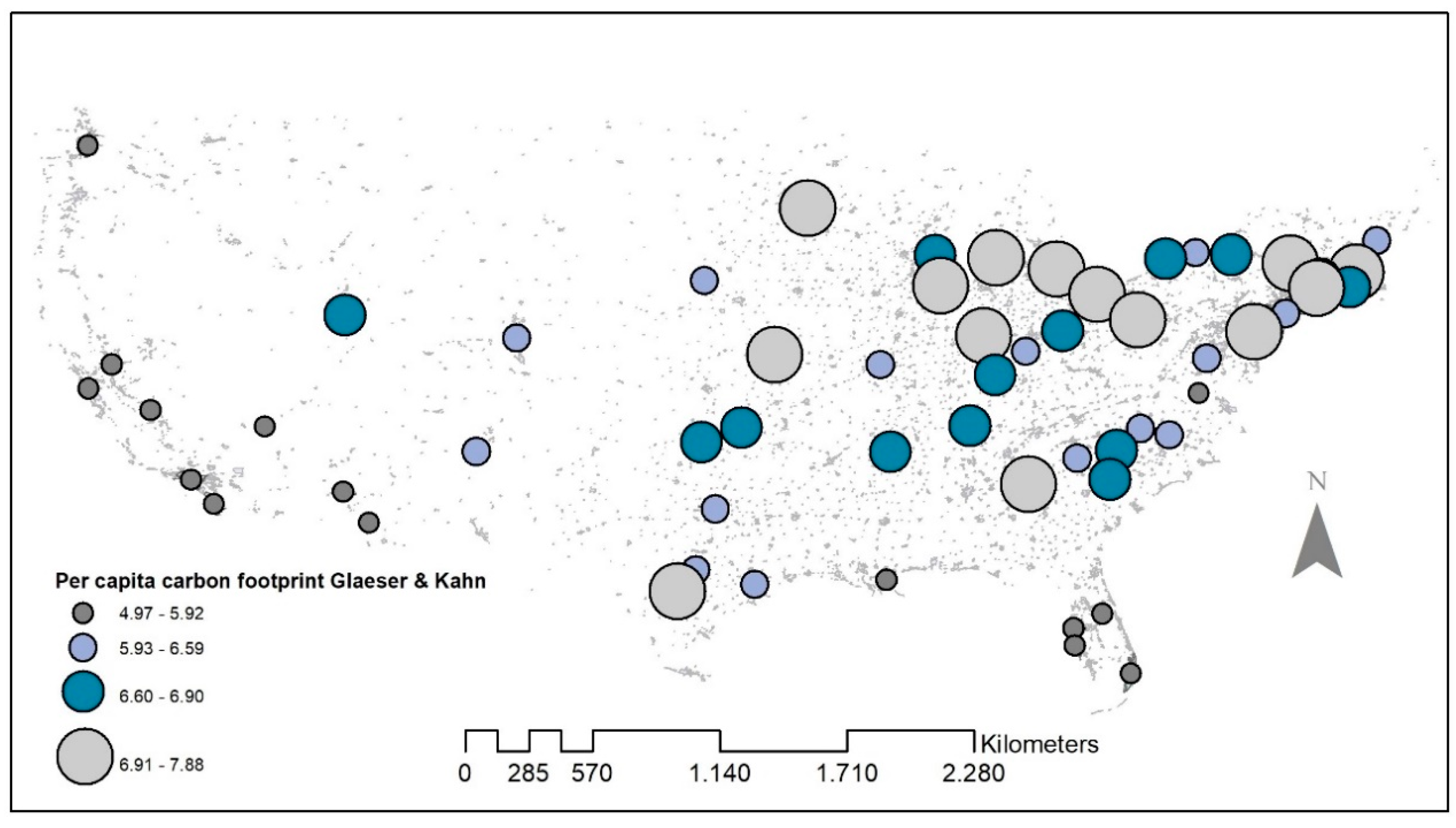
3.1. Location Patterns of Cities with Higher and Lower Carbon Footprint

Despite the differences in magnitude, (.) the correlation between the carbon footprints calculated in Brown et al. [38] and Glaeser and Kahn [44] is positive and statistically significant, 0.57, which indicates that cities with the highest carbon footprint according to the authors of reference [38] tend to follow a pattern similar to those of Glaeser and Kahn [44]. The average of the estimates reported by Glaeser and Kahn [44] is 9.5 tons of CO2 per capita, while that of Brown et al. [38] is 2.1 tons of CO2 per capita. This may be because they use different methodologies, conversion factors, and data sources. This difference is most likely also related to the fact that the authors of Glaeser and Kahn [44] strictly measure the impact of households that live in homes built between 1980 and 2000. As maps in Figure 2 and Figure 3 show, we also find a similar spatial pattern. The cities with the lower per capita carbon footprint are concentrated along the Pacific coast and the northern Atlantic coast. The cities with the highest carbon footprint values tend to be in the Midwest and the south of the country. Figure A1 in Appendix A shows the names of metropolitan areas for easy identification.

3.2. Location Pattern of Cities According to Their Form and Spatial Structure

The densest cities are located on the Atlantic coast (except for San Francisco and Los Angeles) (Figure 4). The most monocentric cities are located in the Midwest and Southwest (Figure 5); the most polycentric cities are located in California (Figure 6) and on the east coast; and the most disperse cities are in the Northeast, South Central, and Southwest (Figure 7).
The values shown in Table 1 indicate that New York remains the densest city in the United States. With 2028 inhabitants per hectare, its density doubles that of another compact city such as San Francisco (955 inhabitants per hectare). On the other hand, the values referring to the indicators of monocentrism, polycentrism, and dispersion indicate that the concentration of employment in CBDs is low. Las Vegas, with a percentage of 28.2 of the total jobs in the region, is the most monocentric city. The employment subcenters of the most polycentric cities only account for between 28 percent and 14 percent of total jobs. In clear contrast to the previous values, in the most dispersed cities of the United States, the weight of employment located outside the CBD and sub-centers exceeds 85 percent.
Certain location patterns emerge when looking at the ranking of cities. The ten densest cities are mainly in the east of the country; the ten most monocentric cities are mainly in the south; and the ten most polycentric and dispersed are distributed evenly throughout the country. On comparing the maps referring to the per capita footprint with those of density and spatial structure, it is observed that on the north-east coast and in the center-north there are dense cities that also have a high carbon footprint. There is also a coincidence in the location pattern of cities with a greater carbon footprint and location patterns of cities with a higher rate of monocentrism, mainly located in the central and central-eastern corridor of the country, from north to south. The greatest discrepancies are observed when comparing the location of the most polycentric metropolitan areas with those with a greater carbon footprint. The greatest similarities occur between the pattern of location of the most dispersed cities and that of the cities with the greatest footprint. The maps and the ranking table offer a first look that allows some patterns to be identified, some connection between carbon footprint and the built environment, but they must be corroborated by estimating a multivariate regression model.

3.3. Urban Form and Spatial Structure as Determinants of Carbon Footprints

The information contained in Table 2 and Table 3 is the result of the estimation of many regression models testing different combinations of control variables and built environment indicators. The value that appears in the cells is the estimated parameter βk. This parameter is the marginal impact of explanatory variable k on the dependent variable (carbon footprint). The value that appears in parentheses is the Student’s “t” indicator. For instance, if it exceeds an absolute value of 1.96 (the confidence interval is 95%) then, the parameter is different from zero.
Population Density. In the case of mobility, a negative correlation is detected. Higher density means lower per capita carbon footprint when using the carbon footprint data from both Glaeser and Kahn [44] and Brown et al. [38]. However, the opposite holds true in housing. Greater density leads to higher emissions, once again using the per capita carbon footprint data from both Glaeser and Kahn [44] and Brown et al. [38]. When using the per capita carbon footprint from both mobility and housing as the dependent variable, either the effect is not significant (with the data from Brown et al. [38]) or it is positive (with the data from Glaeser and Kahn [44]). These results could be because cities that contain more high-density urbanized zones have an older and less energy-efficient housing fleet. In this case, high density per se would not bring environmental advantages in the realm of housing if not accompanied by measures that improve the energy efficiency of the buildings, regional climate alliances, and renewable electricity standards [38,41]. The value of the parameter is low (between 0.0015 and −0.0002) and the most significant effect, with a negative sign, is obtained in the case of mobility (with a Student t of −4.8 (Glaeser and Kahn [44] models) and −5.4 (reference [38] models).
The density variable parameter of the results obtained with the model that takes the sum of carbon footprints of mobility and housing as the dependent variable is not significant (with the footprint data of Brown et al. [38]), or it presents a positive sign (with Glaeser and Kahn [44] data). These results are contrary to those obtained in reference [41] and reference [40] and in line with those obtained in Glaeser and Kahn [44].
Monocentrism. The parameters of the two monocentrism indicators (centrality and CBD) are generally negative, which indicates that the most monocentric cities have advantages in terms of low per capita carbon footprint in mobility and housing. While it is important to note that the parameter always has low statistical significance, the t statistic is in no case higher than 2.6. These results coincide with those obtained in Glaeser and Kahn [44]. Thus, the effect is detected in the realm of housing but not in mobility, an unexpected result given that the concentration of jobs and population in the main urban center facilitates the use of public transport. The negative correlation between the centrality indicators and residential per capita carbon footprint may be because urban centers usually have smaller homes in apartment buildings than in the suburbs. The results obtained using the carbon footprint calculated by Glaeser and Kahn [44] as dependent variable is similar to those obtained using the carbon footprint estimation of Brown et al. [38].
Polycentrism. The correlation between the polycentrism variables (sub-center and polycentrism) and per capita carbon footprint is negative and affects mobility and fuel consumption in households. This correlation is detected with the data from Glaeser and Kahn [44], the data from Brown et al. [38], and the two variables that measure polycentrism. However, it is relevant to point out that none of the parameters that measure polycentrism is significant if the sum of per capita residential and mobility carbon footprint is used as a dependent variable.
Once the existence of environmental advantages associated with polycentrism has been found, we question to what extent the most polycentric cities have a low per capita carbon footprint, not because they are polycentric but because they are larger. There is a positive correlation between population size and the polycentrism indicators used in our study. To discard this possibility, estimations were performed including population size, polycentrism indicators and control variables as regressors. The parameters obtained were altered in value, but their statistical significance was not overly affected, which may indicate that, regardless of the city size, polycentrism may have advantages in terms of low per capita carbon footprint.
Sprawl. Our results indicate that greater sprawl is correlated with a higher volume of emissions from mobility (with the carbon footprint data from Brown et al. [38] and data from Glaeser and Kahn [44]).
The most relevant control variable in this study is total population. Urban size is a widely discussed issue in the debates on bio-regionalism within the Self-Sufficient City Approach. While supporters of the Compact City Approach see no problem associated with mega cities, supporters of the Self-Sufficient City Approach defend a limited urban size based on the limited natural resources of their natural region. The coefficient referring to city size is negative and significant for mobility. A less populous city also tends to occupy a smaller area, which lowers commuting distances compared to large cities, and therefore also lowers the per capita carbon footprint of mobility. However, large cities have more and better public transport infrastructures, which may result in a low per capita carbon footprint. Our results indicate that the “public transport effect” is higher than the “distance traveled effect”. Once again, the results obtained using the emissions data from Glaeser and Kahn [44] and Brown et al. [38] are similar.
The temperature, market regulation index, population size in 1900, and population growth between 1900 and 1930 show a significant correlation with per capita carbon footprint. The coldest cities have a higher per capita carbon footprint since they require more energy to warm their homes. The hottest cities have a high carbon footprint in the summer, since part of the electricity used to operate air conditioners comes from burning fossil fuels. In terms of market regulation, the hypothesis of Glaeser and Kahn [44] states that the cities that regulate land use the most have a greater capacity to accept environmental regulations. The oldest cities (with a higher population in 1900) tend to show a low level of emissions. The urban growth rate between 1900 and 1930 also negatively influences the per capita carbon footprint. Finally, higher per capita income should lead to a higher carbon footprint, since it means higher energy consumption on housing and mobility (larger houses, more and larger cars). However, Glaeser and Kahn [44] and Brown et al. [38] did not detect this correlation, and nor did we. Cities with high per capita income may paradoxically show advantages in terms of low carbon footprint, perhaps because families with a higher income self-select in cities with a low per capita carbon footprint. Taken as a whole, these results seem to indicate that the most dynamic cities in the early 20th century, when their growth was still before the automobile culture, currently have a lower per capita carbon footprint. Therefore, the inertia effects of the built environment must be very persistent over time.
Leaving aside the case of density, manipulation of the spatial structure can have substantial effects for some sub-footprints (see Table A3 in Appendix A). For example, if the centrality index increased by 10%, there would be a fall in the electricity carbon footprint of between 2.43%, with data from Glaeser and Kahn [44], and 3.51%, with data from Brown et al. [38]—an impact that we consider significant. In contrast to the previous case, increasing the polycentrism index by 10% would only reduce the heating carbon footprint by 0.36%, with data from Glaeser and Kahn [44], and 0.7%, with data from Brown et al. [38]. The greatest impact is detected with the dispersion index. Increasing the dispersion index by 10% means an increase of 4.64 in the car’s carbon footprint, with data from Glaeser and Kahn [44] and a 12.2% increase in the heating carbon footprint, with data from Brown et al. [38] (see Table A4 and Table A5 in Appendix A).

4. Discussion

There are differentiated explanations of the lack of statistical significance of the population density variable on total per capita carbon footprint. The first is that population density exerts a negative impact on the carbon footprint of mobility, but exerts a positive impact on the residential footprint, cancelling each other out in the estimation with the total footprint values. The second is that the population with less environmental awareness self-selects in dense cities. The third is that the population that resides in dense cities compensates for the lack of green spaces and excess congestion, with greater leisure mobility during weekends and holidays, which would lead to a greater carbon footprint [33,36,64,65,66]. Another possible explanation is that the density indicator used is not correct. We tested three different density measurements. The first is the gross density of the entire urban region. The second is the density of the central metropolitan subsystem. This value is higher than the previous one. These last two indicators, population density and the population density of the central urban subsystem, are highly correlated. The problem is that they are less significant than the standard gross density, which is why we have not included these models in the results tables.
The policy recommendations which can be gleaned from the results are neither obvious nor direct. Within the tradition of urban planning, these results can be used as an argument to stop the dispersed decentralization of cities. However, within the framework of urban economics, matters are otherwise. Both Gaigné et al. [67] and Glaeser and Kahn [44] argue that compactness policies that seek greater centralization and density may have a perverse effect, since by stopping the growth of urbanized land, families and companies head towards other cities that are more permissive with their physical expansion and less concerned about lowering their GHG emissions. Our position in this regard is in favor of homogeneous environmental regulation upheld by sound information and knowledge. It is not reasonable to think that the free market will solve this kind of problem by allowing the population to “vote with their feet”. Therefore, market regulation seems the best choice.

5. Conclusions

The results of this study confirm that urban form and spatial structure affect the per capita carbon footprint of mobility and housing. However, their impact is modest compared to other control variables, particularly total population, per capita income, and temperature. Even though there are numerous built environment parameters which are significant in the partial models, their statistical significance in the model which takes the sum of emissions from mobility and housing as the dependent variable is negligible. This is partly since they exert an effect in one direction in one partial model and in the opposite direction in another partial model, thereby nullifying each other in the models estimated with total per capita carbon footprint data. These results indicate that a high density and monocentric or polycentric spatial structure are not a guarantee of low carbon footprint if they are not accompanied by specific policies which increase the energy efficiency of housing and promote the use of public transport.
This study has a series of limitations which cannot be ignored. The first is that we estimated the models solely based on the information on large cities. The sample of cities does not include any with a population under 350,000. The second limitation is that we used spatial structure indicators which could be improved. The polycentrism indicators could also include productive specialization and mobility flows to capture not only the urban morphology but also its functionality. In terms of the dispersion indicator, it only includes the spatial behavior of economic activity, ignoring issues like the discontinuity of the built area or the low density of suburban neighborhoods. Nor have we borne in mind other possible spatial structures such as linear, cellular, vertical, or fractal structures, all of which have been subject to debate in the field of urban planning in recent decades. Including these aspects would enrich the analysis, although homogeneous access to all the information needed and for all cities is virtually impossible. The third limitation is that our study is static, when it would be more interesting to question whether the changes in cities’ form and spatial structure give rise to changes in the volume of per capita carbon footprint. A dynamic model would provide the rigor needed to truly discuss causality. The fourth limitation is that we found no adequate instrumental variables to consider all endogeneity issues more effectively. In future work we want to address some of these issues.

Author Contributions

I.M. was in charge of the direction and wrote the manuscript, and contributed to the review and editing process. A.D. was in charge of the econometric strategy, model estimation, and the review and editing in the publication process. Both authors have read and agreed to the published version of the manuscript. All authors have read and agreed to the published version of the manuscript.

Funding

This research received no external funding.

Conflicts of Interest

The authors declare no conflicts of interest.

Appendix A

Table A1. The carbon footprint values calculated by Glaeser and Kahn [44].
Data and SourcesOriginal IndicatorPrimary Conversion FactorsSecondary Conversion FactorsSummary
Mobility. Gas consumption. National Household Transportation survey (NHT) 2001Miles of travel NHT estimates gasoline consumption based on the type of vehicle. From the consumption of gasoline, CO2 emissions are estimated.
Gallons of gasoline:
lbs. CO2 *19,564
To incorporate indirectly emitted CO2, 20% is added to the previous values. Data miles traveled. NHT converts them into gasoline consumption. General model where gasoline consumption is explained by socio-economic variables and characteristics of the ZIP code (population density and distance to the CBD). Consumption of gasoline by a standard family ($62,500 rent and 2.62 members) is estimated for each census tract. Finally, census tracts aggregate metropolitan areas are formed.
Housing.
Heating. Fuel consumption.
Census 2000 IPUM (sample 5%).House owners
and tenant expenditure
Fuel oil 22.39 lbs. of CO2 per gallon.
Natural gas 120.59 CO2 per 100 cubic feet.
To incorporate indirectly emitted CO2, 20% is added to the previous values.With a sub-sample of IPUM for owners who live in the 66 metropolitan areas studied, a regression is carried out where the consumption of fuel oil and natural gas depends on individual characteristics for each metropolitan area. They use the coefficients to estimate the consumption of gas and fuel oil for a family of 2.62 members with an income of $62,500, controlling for individual characteristics and temperature but not for the type of building. CO2 is estimated by applying the conversion factors.
Housing.
Electricity.
Census 2000 IPUM (sample 5%)
North American Electricity Reliability Corporation (NERC).
House owners
and tenant expenditure.
Conversion of electricity expenditure to electricity consumption.Conversion of electricity consumption into CO2 emissions.With a sub-sample of IPUM for owners who live in the 66 metropolitan areas studied, a regression is carried out where electricity consumption depends on individual characteristics for each metropolitan area. They use the coefficients to estimate the consumption of gas and fuel oil for a family of 2.62 members with an income of $62,500, controlling for individual characteristics and temperature but not for the type of building. Consumption spending is converted by considering regional electricity markets.
Primary energy sources are controlled for.
CO2 is estimated by applying the conversion factors
Source: Glaeser and Kahn [44].
Table A2. The carbon footprint values calculated by Brown et al. [38].
Data and SourcesOriginal IndicatorTransformed IndicatorsPrimary Conversion FactorsSecondary Conversion FactorsSummary
Mobility. Gas consumption
Reference [40]
1. Daily Vehicle Miles of travel (DVMT) (Highway Performance Monitoring System (HPMS); Federal Highway national Administration (FHWA); Highway Statistics (FHWA).
2. Conversion into gallons of fuel consumed (Oack Ridge National Laboratory (ORLN); Transportation Energy data Book; FHWA Highway Statistics Publications
Tracks: US Census Bureau 2002 Vehicle Inventory and US Survey (VIVS); FHWA’s Highway Statistics.
Daily Vehicle Miles of travel (DVMT).Gas consumption by cars and small trucks Caloric content of fuels
(Btu/gallon)
Conversion of caloric content into CO2 (TgCO2/QBtu).1. DVMT calculation at urban area scale
2. Rescale at the metropolitan area scale
3. Conversion of fuel consumption into CO2.
Heating Fuel
Reference [39]
EIA (Fuel consumption per household. Census, 2000.
Environmental Protection Agency (EPA) 2007 conversion factors.
Households’ fuel consumption at state level Fuel consumption considering differences in housing typologies.EPA (2007)
CO2/fuel type.
1. Fuel consumption per family at state level.
2. Fuel consumption according to type of housing nationwide.
3. Number of households for each metropolitan area according to housing type.
4. Assign fuel consumption at the metropolitan scale according to the weight of each type of housing in the metropolitan area
5. Fuel consumption at metropolitan scale
6. Conversion of fuel consumption into CO2
Electricity
Reference [39]
Platts Analytics
Census 2000
Brooking Institution
EIA (Annual Energy Outlook)
EIA (state electricity profiles).
Utilities $ and MWh Direct payments Household
and consumption estimation of
households that pay for their electricity consumption in the rental of the property.
Conversion MWh/Btu (10776).Tones CO2/MWh (0.62).1. MWh for each utility in 100-m areas (Platts Analytics).
2. Estimate the number of households with the scope map of the different utilities.
3. Total consumption ZIP code = average consumption per number of households.
4. Aggregation at county level.
5. Adjust consumption included in rentals.
6. Add to metropolitan scale.
7. Convert MWh into CO2 emissions.
Source: Brown et al. [38].
Figure A1. Metropolitan areas. Source: Own elaboration.
Sustainability 12 00389 g0a1
Table A3. Manipulation of the spatial structure Increase of 10%.
VariableObs.MeanStd. Dev.Min.Max.10%
cbd7510.764.932.828.21.08
centrali7434.9814.276.1885.843.50
subcenters757.786.47028.80.78
policentr7426.6917.76059.272.67
dispers7581.476.0362.995.68.15
Source: Own calculations.
Table A4. Spatial structure Increase of 10% and change in dependent variable: results with the estimation in Table 2.
Descriptive Statistics10% Increase in x Variable
VariableObs.MeanStd. Dev.MinMax % ChangeVar. Exp.
Elec. 2583.1641.2361.1075.035−0.083.09−2.43centrali
Auto 3584.7450.6023.1915.860−0.024.73−0.36subcenters
Auto 4584.7450.6023.1915.8600.224.974.64dispers
Source: Own calculations.
Table A5. Spatial structure Increase of 10% and change in dependent variable: results with the estimation in Table 3.
Descriptive Statistics10% Increase in x Variable
VariableObsMeanStd. Dev.MinMax % ChangeVar. Exp.
Elec 1750.7080.2980.161.3−0.0250.683−3.51centrali
Fuel 2750.3330.1940.0220.71−0.0060.326−1.94CBD
Fuel 3750.3330.1940.0220.71−0.0020.330−0.70subcenters
Fuel 4750.3330.1940.0220.710.0410.37312.25dispers
Auto 3751.0780.1760.6641.435−0.0081.070−0.74policentr
Total 2752.1180.4011.2452.804−0.0172.101−0.83centrali
Source: Own calculations.

References

  1. CEC. Green Paper on the Urban Environment; Commission of European Communities: Brussels, Belgium, 1990. [Google Scholar]
  2. Satterthwaite, D. Cities’ contribution to global warming: Notes on the allocation of greenhouse gas emissions. Environ. Urban. 2008, 20, 539–549. [Google Scholar] [CrossRef] [Green Version]
  3. Walraven, A. The Impact of Cities in Terms of Climate Change; United Nations Environment Programme: Paris, France, 2009. [Google Scholar]
  4. Dodman, D. Blaming cities for climate change? An analysis of urban greenhouse gas emissions inventories. Environ. Urban. 2009, 21, 185–201. [Google Scholar] [CrossRef] [Green Version]
  5. Kennedy, C.; Steinberger, J.; Gasson, B.; Hansen, Y.; Hillman, T.; Havránek, M.; Pataki, D.; Ramaswami, A.; Villalba Mendez, G. Greenhouse gas emissions and global cities. Environ. Sci. Technol. 2009, 43, 7297–7302. [Google Scholar] [CrossRef] [PubMed]
  6. Ewing, R.H. Characteristics, causes and effects of urban sprawl: A literature review. In Environment and Urban Issues; FAU/FIU Joint Center: Fort Lauderdale, FL, USA, 1994. [Google Scholar]
  7. Newman, P.W.; Kenworthy, J.R. The land use—Transport connection: An overview. Land Use Policy 1996, 13, 1–22. [Google Scholar] [CrossRef]
  8. Jabareen, Y.R. Sustainable urban forms: Their typologies, models, and concepts. J. Plan. Educ. Res. 2006, 26, 38–52. [Google Scholar] [CrossRef]
  9. ECOTEC. Reducing Transport Emissions through Land Use Planning; Report to the Department of Environment and Department of Transport; HMSO: London, UK, 1993. [Google Scholar]
  10. Levinson, D.; Kumar, A. Activity, travel, and the allocation of time. J. Am. Plan. Assoc. 1995, 61, 458–470. [Google Scholar] [CrossRef]
  11. Ewing, R.; Cervero, R. Travel and the built environment: A synthesis. Transp. Res. Rec. 2001, 1780, 87–114. [Google Scholar] [CrossRef] [Green Version]
  12. Stead, D.; Marshall, S. The relationships between urban form and travel patterns. An international review and evaluation. Eur. J. Transp. Infrastruct. Res. 2001, 1. [Google Scholar] [CrossRef]
  13. Holden, E.; Norland, I.T. Three challenges for the compact city as a sustainable urban form: Household consumption of energy and transport in eight residential areas in the greater Oslo region. Urban Stud. 2005, 42, 2145–2166. [Google Scholar] [CrossRef]
  14. Banister, D. Unsustainable Transport: City Transport in the New Century; Routledge: Abingdon, UK, 2005. [Google Scholar]
  15. Banister, D. Energy, quality of life and the environment: The role of transport. Transp. Rev. 1996, 16, 23–35. [Google Scholar] [CrossRef]
  16. Rong, F. Impact of Urban Sprawl on US Residential Energy. Ph.D. Thesis, School of Public Policy, University of Maryland, College Park, MD, USA, 2006. [Google Scholar]
  17. Ewing, R.; Rong, F. The impact of urban form on US residential energy use. Hous. Policy Debate 2008, 19, 1–30. [Google Scholar] [CrossRef]
  18. Mollay, U. Energy Aware Spatial Planning. Master’s Thesis, Österreichisches Institut für Raumplanung, Viena, Austria, 2010. [Google Scholar]
  19. Cervero, R. Built environments and mode choice: Toward a normative framework. Transp. Res. Part D Transp. Environ. 2002, 7, 265–284. [Google Scholar] [CrossRef]
  20. Giuliano, G.; Narayan, D. Another look at travel patterns and urban form: The US and Great Britain. Urban Stud. 2003, 40, 2295–2312. [Google Scholar] [CrossRef] [Green Version]
  21. Rickwood, P.; Glazebrook, G.; Searle, G. Urban structure and energy—A review. Urban Policy Res. 2008, 26, 57–81. [Google Scholar] [CrossRef] [Green Version]
  22. Marshall, J.D. Energy-efficient urban form. Environ. Sci. Technol. 2008, 42, 3133–3137. [Google Scholar] [CrossRef] [PubMed] [Green Version]
  23. Weisz, H.; Steinberger, J.K. Reducing energy and material flows in cities. Curr. Opin. Environ. Sustain. 2010, 2, 185–192. [Google Scholar] [CrossRef]
  24. Webster, F.V.; Bly, P.H. Changing Pattern of Urban Travel and Implications for Land Use and Transport Strategy; Transportation Research Record; Transportation Research Board: Washington, DC, USA, 1987. [Google Scholar]
  25. Mogridge, M.J.H. Transport, land use and energy interaction. Urban Stud. 1985, 22, 481–492. [Google Scholar] [CrossRef]
  26. Banister, D. Energy use, transport and settlement patterns. In Sustainable Development and Urban Form; Pion: London, UK.
  27. Prevedouros, P.D.; Schofer, J.L. Trip Characteristics and Travel Patterns of Suburban Residents; Transportation Research Record; Transportation Research Board: Washington, DC, USA, 1991. [Google Scholar]
  28. Newman, P.W.; Kenworthy, J.R. Cities and Automobile Dependence: A Sourcebook; Gower: Aldershot, UK, 1989. [Google Scholar]
  29. Newman, P.; Kenworthy, J. Sustainability and Cities: Overcoming Automobile Dependence; Island Press: Washington, DC, USA, 1999. [Google Scholar]
  30. Newman, P.; Kenworthy, J. The end of automobile dependence. In The End of Automobile Dependence; Island Press: Washington, DC, USA, 2015; pp. 201–226. [Google Scholar]
  31. Giuliano, G.; Small, K.A. Is the journey to work explained by urban structure? Urban Stud. 1993, 30, 1485–1500. [Google Scholar] [CrossRef] [Green Version]
  32. Wang, F. Modeling commuting patterns in Chicago in a GIS environment: A job accessibility perspective. Prof. Geogr. 2000, 52, 120–133. [Google Scholar] [CrossRef] [Green Version]
  33. Næss, P. The impacts of job and household decentralization on commuting distances and travel modes: Experiences from the Copenhagen region and other Nordic urban areas. Inf. Raumentwickl. 2007, 2, 149–168. [Google Scholar]
  34. Zhao, P.; Lu, B.; de Roo, G. The impact of urban growth on commuting patterns in a restructuring city: Evidence from Beijing. Pap. Reg. Sci. 2011, 90, 735–754. [Google Scholar] [CrossRef]
  35. Asikhia, M.O.; Nkeki, N.F. Polycentric employment growth and the commuting behaviour in Benin Metropolitan Region, Nigeria. J. Geogr. Geol. 2013, 5, 1. [Google Scholar] [CrossRef]
  36. Muñiz, I.; Calatayud, D.; Dobaño, R. The compensation hypothesis in Barcelona measured through the ecological footprint of mobility and housing. Landsc. Urban Plan. 2013, 113, 113–119. [Google Scholar] [CrossRef]
  37. Lynch, K. A Theory of Good City Form; MIT Press: Cambridge, MA, USA, 1984. [Google Scholar]
  38. Brown, M.; Southworth, F.; Sarzynski, A. Shrinking the Carbon Footprint of Metropolitan America; Brookings Institute: Washington, DC, USA, 2008. [Google Scholar]
  39. Brown, M.A.; Logan, E. The Residential Energy and Carbon Footprints of the 100 Largest U.S. Metropolitan Areas; Georgia Tech Working Paper Series; Georgia Institute of Technology: Atlanta, GA, USA, 2008. [Google Scholar]
  40. Southworth, F.; Sonnenberg, A.; Brown, M.A. The Transportation Energy and Carbon Footprints of the 100 Largest U.S. Metropolitan Areas; Georgia Tech Library, School of Public Policy Working Papers; Georgia Institute of Technology: Atlanta, GA, USA, 2008. [Google Scholar]
  41. Brown, M.; Southworth, F.; Sarzynski, A. The geography of metropolitan carbon footprints. Policy Soc. 2009, 27, 285–304. [Google Scholar] [CrossRef] [Green Version]
  42. Southworth, F.; Sonnenberg, A. Set of comparable carbon footprints for highway travel in metropolitan America. J. Transp. Eng. 2011, 137, 426–435. [Google Scholar] [CrossRef]
  43. Tsai, Y.H. Quantifying urban form: Compactness versus ‘sprawl’. Urban Stud. 2005, 42, 141–161. [Google Scholar] [CrossRef]
  44. Glaeser, E.L.; Kahn, M.E. The greenness of cities: Carbon dioxide emissions and urban development. J. Urban Econ. 2010, 67, 404–418. [Google Scholar] [CrossRef] [Green Version]
  45. Norman, J.; MacLean, H.L.; Kennedy, C.A. Comparing high and low residential density: Life-cycle analysis of energy use and greenhouse gas emissions. J. Urban Plan. Dev. 2006, 132, 10–21. [Google Scholar] [CrossRef]
  46. Van de Weghe, J.R.; Kennedy, C.A. spatial analysis of residential greenhouse gas emissions in the Toronto census metropolitan area. J. Ind. Ecol. 2007, 11, 133–144. [Google Scholar] [CrossRef]
  47. Andrews, C.J. Greenhouse gas emissions along the rural-urban gradient. J. Environ. Plan. Manag. 2008, 51, 847–870. [Google Scholar] [CrossRef]
  48. Veneri, P. Urban polycentricity and the costs of commuting: Evidence from Italian metropolitan areas. Growth Chang. 2010, 41, 403–429. [Google Scholar] [CrossRef]
  49. Muñiz, I.; Garcia-López, M.À. Urban form and spatial structure as determinants of the ecological footprint of commuting. Transp. Res. Part D Transp. Environ. 2019, 67, 334–350. [Google Scholar] [CrossRef]
  50. Muñiz, I.; Sánchez, V. Urban Spatial Form and Structure and Greenhouse-gas Emissions from Commuting in the Metropolitan Zone of Mexico Valley. Ecol. Econ. 2018, 147, 353–364. [Google Scholar] [CrossRef]
  51. Lee, B.; Gordon, P. Urban spatial structure and economic growth in US metropolitan areas. In Proceedings of the 46th Annual Meetings of the Western Regional Science Association, Newport Beach, CA, USA, 29–31 March 2007. [Google Scholar]
  52. McMillen, D.P. Nonparametric employment subcenter identification. J. Urban Econ. 2001, 50, 448–473. [Google Scholar] [CrossRef]
  53. Gordon, P.; Richardson, H.W. Beyond polycentricity: The dispersed metropolis, Los Angeles, 1970–1990. J. Am. Plan. Assoc. 1996, 63, 289–295. [Google Scholar] [CrossRef]
  54. Pfister, N.; Freestone, R.; Murphy, P. Polycentricity or dispersion? Changes in center employment in metropolitan Sydney, 1981 to 1996. Urban Geogr. 2000, 21, 428–442. [Google Scholar] [CrossRef]
  55. Giuliano, G.; Redfearn, C. Not All Sprawl-Evolution of Employment Centers in Los Angeles, 1980–2000; ERSA Conference Papers; European Regional Science Association: Los Angeles, CA, USA, 2005. [Google Scholar]
  56. Lee, B. “Edge” or “edgeless” cities? Urban spatial structure in US metropolitan areas, 1980 to 2000. J. Reg. Sci. 2007, 47, 479–515. [Google Scholar] [CrossRef]
  57. Shearmur, R.; Coffey, W.J.; Dube, C.; Barbonne, R. Intrametropolitan employment structure: Polycentricity, scatteration, dispersal and chaos in Toronto, Montreal and Vancouver, 1996–2001. Urban Stud. 2007, 44, 1713–1738. [Google Scholar] [CrossRef]
  58. Garcia-López, M.A.; Muñiz, I. Employment decentralisation: Polycentricity or scatteration? The case of Barcelona. Urban Stud. 2010, 47, 3035–3056. [Google Scholar] [CrossRef]
  59. Gallo, M.T.; Garrido, R.; Vilar Águila, M. Cambios territoriales en la Comunidad de Madrid: Policentrismo y dispersión. EURE 2010, 36, 5–26. [Google Scholar]
  60. Gilli, F. Sprawl or reagglomeration? The dynamics of employment deconcentration and industrial transformation in Greater Paris. Urban Stud. 2009, 46, 1385–1420. [Google Scholar] [CrossRef] [Green Version]
  61. Hajrasouliha, A.H.; Hamidi, S. The typology of the American metropolis: Monocentricity, polycentricity, or generalized dispersion? Urban Geogr. 2017, 38, 420–444. [Google Scholar] [CrossRef]
  62. Gibson, C. Population of the One Hundred Largest Cities and Other Urban Places in the United States: 1790–1990; Population Division Working Paper No. 27; U.S. Bureau of the Census: Washington, DC, USA, 1998. [Google Scholar]
  63. Gyourko, J.; Saiz, A.; Summers, A. A new measure of the local regulatory environment for housing markets: The Wharton Residential Land Use Regulatory Index. Urban Stud. 2008, 45, 693–729. [Google Scholar] [CrossRef] [Green Version]
  64. Høyer, K.G.; Holden, E. Household consumption and ecological footprints in Norway–does urban form matter? J. Consum. Policy 2003, 26, 327–349. [Google Scholar] [CrossRef]
  65. Holden, E.; Linnerud, K. Troublesome leisure travel: The contradictions of three sustainable transport policies. Urban Stud. 2011, 48, 3087–3106. [Google Scholar] [CrossRef]
  66. Muñiz, I.; Rojas, C. Urban form and spatial structure as determinants of per capita greenhouse gas emissions considering possible endogeneity and compensation behaviors. Environ. Impact Assess. Rev. 2019, 76, 79–87. [Google Scholar] [CrossRef]
  67. Gaigné, C.; Riou, S.; Thisse, J.F. Are compact cities environmentally friendly? J. Urban Econ. 2012, 72, 123–136. [Google Scholar] [CrossRef]
Figure 1. Modeling scheme.
Sustainability 12 00389 g001
Figure 2. Per capita carbon footprint from Glaeser and Kahn [44]. Source: Glaeser and Kahn [44], own calculations.
Sustainability 12 00389 g002
Figure 3. Per capita carbon footprint from Brown et al. [38]. Source: Brown et al. [38], own calculations.
Sustainability 12 00389 g003
Figure 4. Population density. Source: U.S. Census Bureau, own calculations.
Sustainability 12 00389 g004
Figure 5. Percentage of jobs in the Central Business District. Indicator of Monocentrism. Source: Reference [51], own calculations.
Sustainability 12 00389 g005
Figure 6. Percentage of jobs in subcenters. Indicator of polycentrism. Source: Reference [51], own calculations.
Sustainability 12 00389 g006
Figure 7. Percentage of dispersed jobs. Indicator of sprawl. Source: Reference [51], own calculations.
Sustainability 12 00389 g007
Table 1. Ranking of shape/spatial structure indicators (top ten, from highest to lowest).
RankingPopulation Density pop/haMonocentrism (CBD)Polycentrism (Subcenters)Dispersion (Disperse)
1New York 2028.7Las Vegas 28.2L.A. 28.8Allentown 95.6
2Chicago 1322 Birmingham 22.8San Francisco 24.2Orlando 92.1
3Miami 1230Bakersfield 21.7San Diego 22.7Springfield 91.2
4Philadelphia 1042.7Austin 21.5Detroit 22.2Tucson 91
5Providence 1041.5Dayton 20.1Houston 20.8Harrisburg 88.4
6Boston 1034.1Syracuse 19.3Omaha 20.8Greenville 88.3
7San Francisco 955Charleston 16.8Dallas 15.8El Paso 88
8Milwaukee 942.3New Orleans 16.7San Antonio 15.6Albuquerque 87
9Tampa 938.1Omaha 16.4Miami 15Cleveland 87
10Detroit 831.1Columbia 16.3Norfolk 14.3Buffalo 86.9
Source: U.S. Census Bureau and reference [51].
Table 2. Results of Glaeser and Kahn [44]. Dependent variable: t CO2 per capita.
Urban Model VariablesElec 1Elec 2Fuel 1Fuel 2Auto 1Auto 2Auto 3Auto 4Total
Population 0.0003
(3.0)
−0.00005
(−3.0)
Density0.0009
(2.3)
0.0003
(1.93)
−0.0002
(−4.8)
0.0015
(2.3)
CBD
Centrali −0.022
(−2.14)
Subcentre −0.022
(−2.6)
Policentri
Dispers 0.027
(2.6)
Control Variables
IncomeYesYesYesYesYesYesYesYesYes
TempYesYesYesYesYesYesYesYesYes
CoastYesYesYesYesYesYesYesYesYes
RegulationYes Yes
Historic population growth YesYesYesYes
Pop 1900 Yes
No. obs.585745455845455858
Adj. R20.450.270.700.690.540.560.510.440.31
Source: Own calculations.
Table 3. Results of Brown et al. [38]. Dependent variable: t CO2 per capita.
Urban Model VariablesElect 1Fuel 1Fuel 2Fuel 3Fuel 4Auto 1Auto 2Auto 3Total 1Total 2
Population −0.00002
(−4.47)
−0.00003
(−1.98)
Density 0.00009
(2.18)
−0.0003
(−5.42)
CBD −0.006
(−2.05)
Centrali−0.0071
(−2.6)
−0.005
(−2.29)
subcentres −0.003
(−2.16)
policentri −0.003
(−2.13)
dispers 0.005
(2.43)
Control Variables
GDPYesYesYesYesYesYesYesYesYesYes
TempYesYesYesYesYesYesYesYesYesYes
Coast Yes
RegulationYes YesYes
Historic population growthYesYes Yes Yes
Pop 1900 Yes Yes
No. obs.53547575757554745474
Adj. R20.480.710.560.640.650.230.360.310.480.44
Source: Own calculations.

