Toxic Income as a Trigger of Climate Change


Abstract
:1. Introduction
Toxic Income
2. Data
Methodology
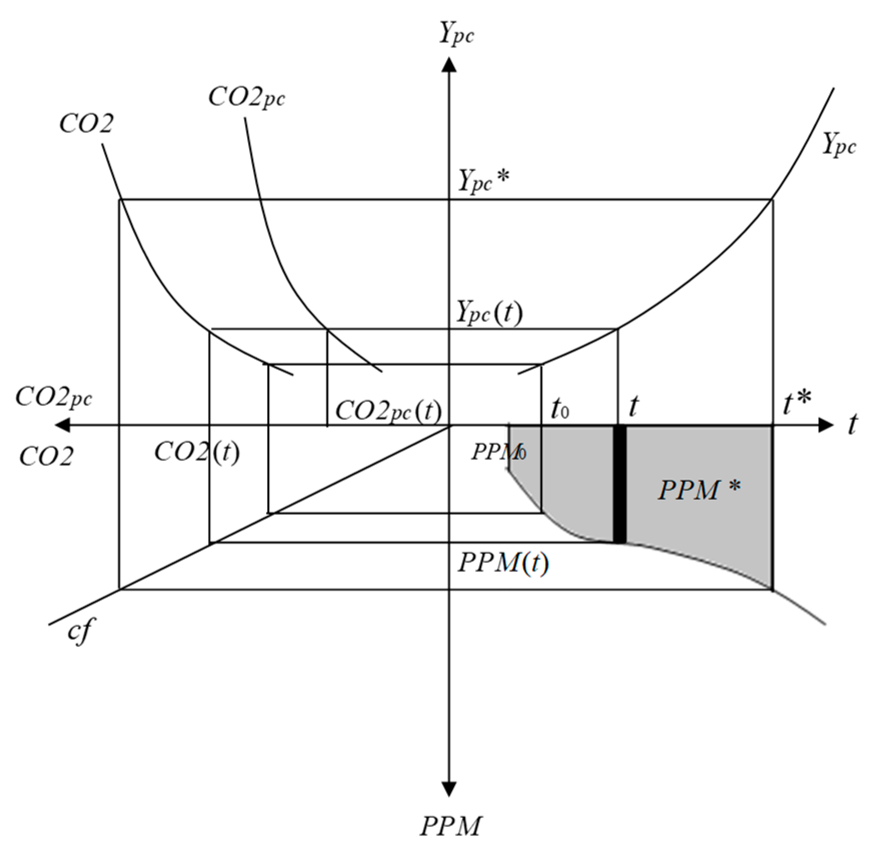
- is the time index;
- is per capita CO2 emissions;
- is per capita GDP in year ;
- is the income threshold between the two sections of the regression;
- is energy efficiency defined as: GDP/energy consumption; and
- is the stochastic error with mean value of zero and constant variance.
- First, we verified that emissions per capita and income per capita were co-integrated. For all countries, both time series were integrated of order 1, , with the exception of China, whose time series were integrated of order 2, . Then, the parameters were estimated using ordinary least squares (OLS). All econometric equations generated stationary residual at 5% level except for China and the Democratic Republic of Congo, whose residual were stationary at 10% level of significance. Therefore, the estimated parameters by OLS continued having good properties. In fact, the estimators were super consistent; they converged to the true value at a rate 1/T, instead of the habitual convergence ratio [34].
- For low income countries, we applied only the linear model; for lower-middle income countries, we selected between the linear and the linear spline model. In both cases, the assumption is made of a positive relation between CO2 emissions and income. For upper middle and high income countries, we selected among the three models. The final section of the econometric function may have a positive, negative, or null slope, for those countries. The selection of the final model to be used was linked to the lowest value for the Akaike Information Criterion (AIC).
- In the case of spline regression models, for each value of income, , a regression was estimated, and then the income threshold was computed minimizing the Akaike information criterion, that is, .
- Additionally, errors autocorrelation was verified. In the presence of autocorrelation, the correction term AR (1) was applied.
- Finally, we only included countries with a coefficient of determination larger than 0.6.
3. Results and Discussion
3.1. Results by Income Group
3.2. Estimated Toxic Income
3.3. Historical Responsibilities Related to Toxic Income
4. Conclusions and Policy Implications
Author Contributions
Funding
Acknowledgments
Conflicts of Interest
Appendix A. Econometric Regressions

| Country | AIC | ndat | ||||||
|---|---|---|---|---|---|---|---|---|
| Ethiopia | 0.913 | 0.067 | 4.248 | −2.050 | 2.211 | −7.434 | 34 | |
| 7.421 | 7.191 | −6.817 | ||||||
| Benin | 0.921 | −1.000 | 2.445 | −0.191 | 0.304 | 2.009 | −3.181 | 44 |
| −8.684 | 14.721 | −3.239 | 2.175 | |||||
| Congo, Dem. Rep. | 0.949 | −0.014 | 0.283 | −0.038 | 0.703 | 2.133 | −5.983 | 44 |
| −1.053 | 5.117 | −2.214 | 5.333 | |||||
| Mozambique | 0.751 | −0.007 | 3.340 | −1.224 | 0.423 | 1.723 | −4.116 | 35 |
| −0.221 | 7.395 | −7.391 | 1.647 | |||||
| Nepal | 0.909 | −0.081 | 0.905 | −0.162 | 0.740 | 1.634 | −4.923 | 44 |
| −1.412 | 5.579 | −1.971 | 6.781 |
| Country | AIC | ndat | ||||||
|---|---|---|---|---|---|---|---|---|
| El Salvador | 0.760 | 0.095 | 0.554 | −0.197 | 2.656 | −1.005 | 44 | |
| 0.499 | 11.091 | −4.041 | ||||||
| Guatemala | 0.789 | −0.357 | 0.552 | −0.070 | 0.284 | 2.114 | −1.921 | 44 |
| −0.830 | 5.905 | −1.304 | 1.907 | |||||
| Indonesia | 0.931 | 0.191 | 0.699 | −0.138 | 0.312 | 1.627 | −0.898 | 44 |
| 0.422 | 6.015 | −0.709 | 4.062 |
| Country | AIC | ndat | ||||||||
|---|---|---|---|---|---|---|---|---|---|---|
| Bangladesh | 0.997 | 0.103 | 0.887 | 0.707 | −0.093 | 0.551 | 1.651 | −7.073 | 43 | |
| 2.766 | 55.419 | 33.485 | −8.541 | |||||||
| Bolivia | 0.868 | −1.444 | 2.042 | 0.928 | −0.158 | 1.466 | 2.121 | −1.042 | 44 | |
| −2.297 | 4.537 | 8.135 | −7.702 | |||||||
| Cote d’Ivoire | 0.651 | −0.823 | 1.069 | 0.040 | −0.049 | 1.527 | 1.573 | −2.106 | 44 | |
| −3.856 | 4.893 | 0.569 | −1.485 | |||||||
| Honduras | 0.792 | 0.521 | 0.069 | 1.202 | −0.037 | 1.498 | 2.354 | −1.520 | 44 | |
| 0.815 | 0.107 | 10.440 | −0.243 | |||||||
| Mongolia | 0.796 | 4.920 | 1.647 | 4.705 | −2.713 | 2.229 | 2.186 | 3.055 | 30 | |
| 3.418 | 1.792 | 8.090 | −3.673 | |||||||
| Morocco | 0.993 | 0.728 | 0.696 | 0.515 | −0.173 | 2.508 | 1.892 | −3.798 | 44 | |
| 6.363 | 51.437 | 12.178 | −8.261 | |||||||
| Myanmar | 0.801 | 0.078 | 0.928 | 0.572 | −0.158 | 0.347 | 1.667 | −4.331 | 44 | |
| 3.987 | 6.368 | 6.081 | −5.037 | |||||||
| Pakistan | 0.994 | 0.226 | 1.380 | 0.654 | −0.340 | 1.014 | 2.017 | −5.075 | 44 | |
| 2.865 | 35.227 | 2.700 | −5.973 | |||||||
| Tunisia | 0.988 | 0.988 | 0.919 | 0.540 | −0.346 | 2.110 | 2.136 | −2.840 | 44 | |
| 2.432 | 11.115 | 23.957 | −5.186 | |||||||
| Egypt, Arab Rep. | 0.975 | 0.954 | 0.760 | 1.021 | −0.246 | 0.388 | 1.513 | 1.922 | −1.803 | 44 |
| 1.741 | 2.635 | 14.121 | −2.669 | 3.442 | ||||||
| India | 0.997 | 0.269 | 2.478 | 1.362 | −0.584 | 0.242 | 0.657 | 1.833 | −4.773 | 44 |
| 3.500 | 17.217 | 17.105 | −7.541 | 2.353 | ||||||
| Sri Lanka | 0.964 | 0.140 | 0.455 | 0.345 | −0.107 | 0.618 | 1.947 | 2.485 | −3.567 | 44 |
| 1.894 | 6.736 | 7.876 | −2.925 | 3.938 |
| Country | AIC | ndat | |||||
|---|---|---|---|---|---|---|---|
| Argentina | 0.872 | 2.470 | 0.333 | −0.253 | 2.449 | −0.952 | 44 |
| 6.893 | 14.607 | −2.880 | |||||
| Ecuador | 0.753 | 0.857 | 0.645 | −0.247 | 1.743 | 0.314 | 44 |
| 1.460 | 8.749 | −3.610 | |||||
| Mexico | 0.934 | 4.185 | 0.368 | −0.589 | 1.742 | −1.040 | 44 |
| 12.263 | 19.784 | −11.287 |
| Country | AIC | ndat | ||||||||
|---|---|---|---|---|---|---|---|---|---|---|
| Costa Rica | 0.936 | 0.446 | 0.274 | 0.046 | −0.078 | 6.606 | 2.348 | −1.954 | 44 | |
| 1.303 | 11.236 | 1.913 | −2.841 | |||||||
| Panama | 0.848 | 0.896 | 0.545 | 0.292 | −0.304 | 6.523 | 2.308 | −0.538 | 44 | |
| 5.389 | 10.185 | 7.270 | −8.757 | |||||||
| South Africa | 0.896 | 4.491 | 1.996 | 0.828 | −3.181 | 6.217 | 2.045 | 0.492 | 44 | |
| 3.174 | 7.541 | 7.983 | −17.026 | |||||||
| Turkey | 0.997 | 1.845 | 0.459 | 0.324 | −0.327 | 0.513 | 8.332 | 1.967 | −2.544 | 55 |
| 6.061 | 29.324 | 17.580 | −9.248 | 3.240 |
| Country | AIC | ndat | |||||||||
|---|---|---|---|---|---|---|---|---|---|---|---|
| Albania | 0.895 | 0.181 | 2.784 | −0.446 | 1.149 | −0.749 | 3.001 | 2.064 | 0.203 | 35 | |
| 0.182 | 3.186 | −2.203 | 7.376 | −13.06 | |||||||
| Algeria | 0.644 | −5.021 | 4.907 | −0.696 | 1.249 | −0.134 | 4.091 | 2.065 | 0.816 | 44 | |
| −1.466 | 2.516 | −2.446 | 2.567 | −3.752 | |||||||
| Botswana | 0.910 | 4.127 | −1.503 | 0.389 | 0.544 | −0.567 | 4.011 | 1.835 | −0.412 | 34 | |
| 3.183 | −1.608 | 2.729 | 5.605 | −3.890 | |||||||
| Brazil | 0.938 | 0.734 | 0.806 | −0.037 | 0.266 | −0.395 | 9.762 | 1.854 | −1.865 | 44 | |
| 1.317 | 3.918 | −2.836 | 8.088 | −5.648 | |||||||
| Bulgaria | 0.931 | −121.8 | 77.278 | −10.73 | 2.716 | −6.991 | 3.782 | 2.351 | 1.502 | 35 | |
| −2.318 | 2.610 | −2.582 | 13.685 | −16.77 | |||||||
| Dominican Republic | 0.951 | 3.399 | −2.130 | 0.630 | 0.204 | −0.189 | 3.194 | 1.776 | −1.351 | 44 | |
| 3.804 | −2.737 | 4.329 | 2.632 | −3.330 | |||||||
| Gabon | 0.714 | 35.089 | −7.053 | 0.413 | 0.292 | −0.352 | 12.131 | 1.985 | 3.506 | 44 | |
| 1.937 | −1.985 | 2.461 | 1.688 | −2.482 | |||||||
| Iran, Islamic Rep. | 0.880 | 9.644 | −2.986 | 0.471 | 0.450 | −0.498 | 5.964 | 2.525 | 1.938 | 44 | |
| 1.950 | −1.471 | 2.306 | 2.050 | −9.868 | |||||||
| Jamaica | 0.878 | 844.7 | −470.6 | 66.019 | 0.297 | −0.947 | 3.674 | 1.652 | 0.086 | 44 | |
| 2.320 | −2.311 | 2.320 | 3.487 | −13.354 | |||||||
| Jordan | 0.969 | 4.225 | −0.198 | 0.181 | 0.261 | −0.709 | 3.349 | 2.540 | −1.434 | 40 | |
| 5.463 | −0.367 | 1.816 | 1.416 | −21.15 | |||||||
| Malaysia | 0.988 | 2.654 | −0.934 | 0.241 | 0.747 | −0.047 | 5.500 | 2.380 | 0.228 | 44 | |
| 2.367 | −2.584 | 5.429 | 19.695 | −0.264 | |||||||
| Mauritius | 0.998 | 0.596 | 0.739 | −0.013 | 0.362 | −0.310 | 6.747 | 2.025 | −3.025 | 39 | |
| 3.934 | 13.067 | −2.185 | 11.702 | −8.939 | |||||||
| Paraguay | 0.891 | 0.720 | −0.173 | 0.142 | 0.332 | −0.172 | 2.912 | 1.652 | −2.486 | 44 | |
| 2.808 | −0.538 | 2.121 | 3.203 | −2.851 | |||||||
| Peru | 0.922 | 2.506 | −0.935 | 0.203 | 0.322 | −0.080 | 4.070 | 2.677 | −2.013 | 44 | |
| 2.717 | −1.723 | 2.496 | 7.972 | −5.417 | |||||||
| Thailand | 0.996 | 0.746 | 0.481 | 0.105 | 0.585 | −0.279 | 3.969 | 1.828 | −1.911 | 44 | |
| 5.344 | 2.760 | 3.029 | 14.106 | −3.696 | |||||||
| China | 0.944 | 1.296 | 5.599 | −0.906 | 1.569 | −2.807 | 0.788 | 2.259 | 1.456 | −1.058 | 44 |
| 3.205 | 6.536 | −3.451 | 16.266 | −10.03 | 4.094 | ||||||
| Colombia | 0.773 | −0.662 | 1.550 | −0.152 | 0.440 | −0.245 | 0.299 | 4.862 | 1.986 | −2.377 | 44 |
| −0.685 | 3.304 | −2.686 | 10.182 | −9.132 | 1.805 | ||||||
| Cuba | 0.810 | −10.857 | 9.691 | −1.537 | 0.963 | −0.621 | 0.263 | 3.473 | 1.909 | −0.306 | 44 |
| −1.282 | 1.756 | −1.730 | 7.750 | −8.657 | 1.720 |
| Country | AIC | ndat | ||||||||
|---|---|---|---|---|---|---|---|---|---|---|
| Israel | 0.958 | 1.714 | 0.450 | 0.009 | −0.424 | 25.509 | 1.835 | 0.798 | 44 | |
| 2.027 | 25.738 | 0.234 | −5.058 | |||||||
| Oman | 0.666 | 9.153 | −0.150 | 2.163 | −0.066 | 15.473 | 2.275 | 4.825 | 44 | |
| 2.265 | −0.537 | 6.245 | −2.058 | |||||||
| Trinidad and Tobago | 0.975 | 17.319 | 0.013 | 2.085 | −2.459 | 7.198 | 2.515 | 3.622 | 44 | |
| 2.274 | 0.012 | 24.748 | −6.239 | |||||||
| United Kingdom | 0.962 | 14.051 | 0.076 | 0.310 | −0.846 | 34.442 | 1.748 | 0.245 | 55 | |
| 82.263 | 4.944 | 7.320 | −13.792 | |||||||
| Uruguay | 0.928 | 2.838 | 0.329 | 0.053 | −0.403 | 9.439 | 2.068 | −1.548 | 44 | |
| 23.158 | 15.428 | 3.085 | −19.476 | |||||||
| Hong Kong SAR, China | 0.970 | 1.992 | 0.411 | 0.173 | −0.278 | 0.513 | 13.191 | 1.914 | 0.149 | 44 |
| 1.521 | 4.085 | 11.037 | −9.293 | 3.570 | ||||||
| Netherlands | 0.929 | 16.579 | 0.156 | 0.254 | −1.476 | 0.207 | 32.148 | 1.979 | 1.114 | 55 |
| 17.995 | 8.061 | 10.476 | −16.966 | 2.032 | ||||||
| Switzerland | 0.923 | 11.825 | −0.002 | 0.068 | −0.320 | 0.267 | 67.385 | 1.973 | −0.790 | 35 |
| 13.043 | −0.207 | 2.037 | −6.161 | 1.446 |
| Country | AIC | ndat | |||||||||
|---|---|---|---|---|---|---|---|---|---|---|---|
| Austria | 0.958 | 10.542 | 0.350 | −0.002 | 0.081 | −1.214 | 44.029 | 1.921 | 0.036 | 55 | |
| 15.634 | 14.285 | −4.544 | 2.191 | −15.016 | |||||||
| Canada | 0.963 | 11.256 | 1.290 | −0.016 | 0.508 | −4.495 | 35.648 | 1.738 | 0.926 | 55 | |
| 3.627 | 8.292 | −5.467 | 12.441 | −12.682 | |||||||
| Chile | 0.958 | 1.943 | 1.705 | −0.134 | 0.385 | −0.831 | 6.309 | 1.655 | −0.205 | 44 | |
| 0.847 | 1.762 | −1.472 | 16.860 | −7.380 | |||||||
| Cyprus | 0.994 | 3.452 | 0.626 | −0.011 | 0.241 | −0.665 | 22.560 | 2.403 | −1.545 | 40 | |
| 11.679 | 15.223 | −8.821 | 29.469 | −28.514 | |||||||
| Denmark | 0.970 | 15.441 | 0.122 | 0.002 | 0.156 | −1.112 | 50.262 | 2.098 | 0.618 | 55 | |
| 12.761 | 2.060 | 2.232 | 6.115 | −25.735 | |||||||
| France | 0.920 | −1.365 | 1.376 | −0.029 | 0.094 | −0.794 | 31.853 | 0.663 | 1.034 | 55 | |
| −0.814 | 13.615 | −13.286 | 2.704 | −5.810 | |||||||
| Greece | 0.983 | 20.967 | −0.891 | 0.021 | 0.243 | −0.629 | 15.738 | 2.562 | 0.726 | 55 | |
| 11.643 | −3.632 | 2.040 | 17.648 | −15.459 | |||||||
| Japan | 0.984 | 8.238 | 0.328 | −0.002 | 0.946 | −0.850 | 44.394 | 2.137 | 0.259 | 55 | |
| 13.181 | 14.006 | −4.428 | 9.250 | −16.436 | |||||||
| Korea, Rep. | 0.996 | 8.486 | 0.440 | 0.067 | 0.450 | −2.072 | 5.405 | 1.938 | 0.026 | 44 | |
| 9.252 | 1.261 | 1.496 | 51.835 | −12.215 | |||||||
| Luxembourg | 0.938 | −43.958 | 5.207 | −0.074 | 0.321 | −3.170 | 43.986 | 2.112 | 4.168 | 55 | |
| −2.227 | 4.665 | −4.721 | 7.387 | −9.767 | |||||||
| Malta | 0.983 | 2.711 | 0.615 | −0.008 | 0.230 | −0.486 | 13.333 | 1.983 | −0.165 | 44 | |
| 7.976 | 6.207 | −1.435 | 9.519 | −15.029 | |||||||
| New Zealand | 0.886 | 10.302 | −0.206 | 0.010 | −0.074 | −0.672 | 30.363 | 1.734 | 0.859 | 38 | |
| 1.431 | −0.390 | 1.020 | −1.127 | −5.208 | |||||||
| Portugal | 0.967 | 5.622 | 0.768 | −0.038 | 0.155 | −0.555 | 12.667 | 1.794 | 0.664 | 55 | |
| 5.856 | 3.508 | −2.952 | 7.536 | −8.153 | |||||||
| Singapore | 0.664 | 6.093 | 1.129 | −0.026 | 0.329 | −0.668 | 38.117 | 1.905 | 4.048 | 44 | |
| 2.407 | 6.636 | −6.857 | 2.237 | −2.060 | |||||||
| United States | 0.966 | 1.001 | 2.143 | −0.032 | 0.531 | −4.161 | 31.269 | 1.800 | 0.628 | 55 | |
| 0.469 | 13.448 | −9.796 | 18.080 | −21.608 | |||||||
| Australia | 0.980 | 15.323 | 0.017 | 0.011 | 0.303 | −1.770 | 0.374 | 31.939 | 2.190 | 1.138 | 55 |
| 2.377 | 0.038 | 1.339 | 6.550 | −5.857 | 2.779 | ||||||
| Belgium | 0.920 | 6.111 | 1.283 | −0.025 | 0.145 | −1.710 | 0.533 | 29.914 | 1.925 | 1.187 | 55 |
| 1.747 | 4.442 | −4.066 | 4.451 | −12.347 | 6.090 | ||||||
| Finland | 0.962 | 12.515 | 1.035 | −0.015 | 0.372 | −3.604 | 0.572 | 29.783 | 2.146 | 1.467 | 55 |
| 4.434 | 4.110 | −2.651 | 10.338 | −14.972 | 3.370 | ||||||
| Ireland | 0.987 | 6.944 | 0.444 | −0.003 | 0.304 | −0.853 | 0.215 | 48.672 | 1.963 | −0.686 | 45 |
| 21.229 | 17.876 | −7.108 | 9.762 | −30.418 | 1.438 | ||||||
| Italy | 0.948 | 28.179 | −1.720 | 0.056 | 0.203 | −1.064 | 0.735 | 22.421 | 2.606 | 0.898 | 55 |
| 7.205 | −3.829 | 4.341 | 6.749 | −19.555 | 6.321 | ||||||
| Norway | 0.835 | 8.743 | 0.341 | −0.002 | 0.183 | −1.061 | 0.754 | 70.458 | 1.935 | 2.745 | 55 |
| 1.604 | 1.486 | −0.862 | 1.970 | −6.057 | 8.580 | ||||||
| Spain | 0.966 | 15.863 | −0.265 | 0.008 | 0.415 | −0.848 | 0.439 | 29.008 | 2.219 | 0.729 | 55 |
| 11.514 | −2.816 | 3.550 | 3.130 | −15.830 | 3.166 | ||||||
| Sweden | 0.955 | −15.067 | 2.484 | −0.047 | 0.200 | −1.266 | 0.443 | 35.239 | 2.020 | 1.228 | 55 |
| −4.588 | 11.399 | −11.995 | 5.843 | −9.595 | 3.312 |
Appendix B
| Business as Usual Scenario | COP 21 Scenario | ||||||||||||
|---|---|---|---|---|---|---|---|---|---|---|---|---|---|
| Year | Popul Mill | PIBpc US$ | CO2pc t | CO2 Gt | GHG Gt | CO2 ppm | GHG ppm | PIBpc US$ | CO2pc t | CO2 Gt | GHG Gt | CO2 ppm | GHG ppm |
| 2014 | 7269 | 10.1 | 5.0 | 36.1 | 54.7 | 397.5 | 440.9 | 10.1 | 5.0 | 36.1 | 54.7 | 397.5 | 440.9 |
| 2015 | 7355 | 10.3 | 5.1 | 37.4 | 56.6 | 399.9 | 444.6 | 10.3 | 5.1 | 37.7 | 57.0 | 399.9 | 444.7 |
| 2016 | 7442 | 10.5 | 5.2 | 38.5 | 58.3 | 402.3 | 448.5 | 10.5 | 5.2 | 38.7 | 58.6 | 402.3 | 448.6 |
| 2017 | 7550 | 10.8 | 5.4 | 39.2 | 59.3 | 404.8 | 452.5 | 10.8 | 5.5 | 39.3 | 59.5 | 404.8 | 452.5 |
| 2018 | 7633 | 11.0 | 5.5 | 40.1 | 60.6 | 407.3 | 456.5 | 11.0 | 5.5 | 40.2 | 60.8 | 407.3 | 456.6 |
| 2019 | 7715 | 11.2 | 5.5 | 41.0 | 62.0 | 409.9 | 460.7 | 11.1 | 5.4 | 40.0 | 60.6 | 409.9 | 460.7 |
| 2020 | 7795 | 11.4 | 5.6 | 41.9 | 63.5 | 412.5 | 464.9 | 11.2 | 5.3 | 39.8 | 60.3 | 412.4 | 464.7 |
| 2021 | 7875 | 11.6 | 5.7 | 42.9 | 65.0 | 415.2 | 469.2 | 11.3 | 5.2 | 39.6 | 59.9 | 414.9 | 468.7 |
| 2022 | 7954 | 11.8 | 5.7 | 43.9 | 66.5 | 418.0 | 473.7 | 11.4 | 5.1 | 39.2 | 59.4 | 417.3 | 472.6 |
| 2023 | 8032 | 12.0 | 5.8 | 45.0 | 68.1 | 420.8 | 478.2 | 11.6 | 5.0 | 38.9 | 58.8 | 419.8 | 476.6 |
| 2024 | 8110 | 12.2 | 5.9 | 46.1 | 69.8 | 423.7 | 482.9 | 11.7 | 4.9 | 38.5 | 58.2 | 422.2 | 480.4 |
| 2025 | 8186 | 12.5 | 6.0 | 47.3 | 71.5 | 426.7 | 487.7 | 11.8 | 4.8 | 38.0 | 57.5 | 424.6 | 484.3 |
| 2026 | 8261 | 12.7 | 6.1 | 48.5 | 73.3 | 429.8 | 492.6 | 12.0 | 4.8 | 38.3 | 57.9 | 427.0 | 488.1 |
| 2027 | 8335 | 12.9 | 6.2 | 49.7 | 75.2 | 432.9 | 497.6 | 12.1 | 4.8 | 38.6 | 58.4 | 429.5 | 492.0 |
| 2028 | 8408 | 13.2 | 6.3 | 51.0 | 77.2 | 436.1 | 502.7 | 12.2 | 4.7 | 38.8 | 58.8 | 431.9 | 496.0 |
| 2029 | 8480 | 13.5 | 6.4 | 52.4 | 79.3 | 439.4 | 508.0 | 12.4 | 4.7 | 39.1 | 59.2 | 434.4 | 499.9 |
| 2030 | 8551 | 13.7 | 6.5 | 53.8 | 81.4 | 442.8 | 513.5 | 12.5 | 4.7 | 39.4 | 59.6 | 436.8 | 503.9 |
| 2031 | 8621 | 13.9 | 6.5 | 54.6 | 82.6 | 446.3 | 519.0 | 12.7 | 4.7 | 39.9 | 60.3 | 439.4 | 507.9 |
| 2032 | 8691 | 14.0 | 6.6 | 55.4 | 83.8 | 449.7 | 524.6 | 12.8 | 4.8 | 40.4 | 61.1 | 441.9 | 512.0 |
| 2033 | 8759 | 14.2 | 6.6 | 56.2 | 85.0 | 453.3 | 530.2 | 13.0 | 4.8 | 40.8 | 61.8 | 444.5 | 516.1 |
| 2034 | 8826 | 14.4 | 6.7 | 57.0 | 86.2 | 456.9 | 536.0 | 13.1 | 4.8 | 41.3 | 62.6 | 447.1 | 520.3 |
| 2035 | 8893 | 14.5 | 6.7 | 57.8 | 87.4 | 460.5 | 541.8 | 13.3 | 4.8 | 41.8 | 63.3 | 449.7 | 524.5 |
| 2036 | 8958 | 14.7 | 6.8 | 58.6 | 88.6 | 464.2 | 547.7 | 13.43 | 4.9 | 42.3 | 64.1 | 452.4 | 528.8 |
| 2037 | 9023 | 14.9 | 6.8 | 59.4 | 89.9 | 468.0 | 553.7 | 13.6 | 4.9 | 42.8 | 64.8 | 455.1 | 533.1 |
| 2038 | 9086 | 15.0 | 6.9 | 60.2 | 91.1 | 471.8 | 559.8 | 13.7 | 4.9 | 43.3 | 65.6 | 457.8 | 537.5 |
| 2039 | 9149 | 15.2 | 6.9 | 61.0 | 92.3 | 475.6 | 566.0 | 13.9 | 4.9 | 43.9 | 66.4 | 460.6 | 541.9 |
| 2040 | 9210 | 15.4 | 7.0 | 61.8 | 93.6 | 479.5 | 572.2 | 14.1 | 5.0 | 44.4 | 67.1 | 463.4 | 546.4 |
References
- Rogelj, J.; Hare, W.; Lowe, J.; van Vuuren, D.P.; Riahi, K.; Matthews, B.; Hanaoka, T.; Jiang, K.; Meinshausen, M. Emission pathways consistent with a 2 °C global temperature limit. Nat. Clim. Chang. 2011, 1, 413–418. [Google Scholar] [CrossRef]
- Den Elzen, M.; Meinshausen, M. Meeting the EU 2°C climate target: global and regional emission implications. Clim. Policy 2006, 6, 545–564. [Google Scholar] [CrossRef]
- Meinshausen, M.; Meinshausen, N.; Hare, W.; Raper, S.C.B.; Frieler, K.; Knutti, R.; Frame, D.J.; Allen, M.R. Greenhouse-gas emission targets for limiting global warming to 2 degrees C. Nature 2009, 458, 1158–1162. [Google Scholar] [CrossRef] [PubMed]
- Rogelj, J.; Hare, B.; Nabel, J.; Macey, K.; Schaeffer, M.; Markmann, K.; Meinshausen, M. Halfway to Copenhagen, no way to 2 °C. Nat. Reports Clim. Chang. 2009, 3, 81–83. [Google Scholar] [CrossRef]
- Guivarch, C.; Hallegatte, S. 2C or not 2C? Glob. Environ. Chang. 2013, 23, 179–192. [Google Scholar] [CrossRef] [Green Version]
- Climate Change 2013: The Physical Science Basis. Contribution of Working Group I to the Fifth Assessment Report of the Intergovernmental Panel on Climate Change; Stocker, T.F.; Qin, D.; Plattner, G.-K.; Tignor, M.; Allen, S.K.; Boschung, J.; Nauels, A.; Xia, Y.; Bex, V.; Midgley, P.M. (Eds.) Cambridge University Press: Cambridge, UK, 2013. [Google Scholar]
- Boykoff, M.T.; Frame, D.; Randalls, S. Discursive stability meets climate instability: A critical exploration of the concept of “climate stabilization” in contemporary climate policy. Glob. Environ. Chang. 2010, 20, 53–64. [Google Scholar] [CrossRef]
- Cleveland, C.J.; Costanza, R.; Hall, C.A.S.; Kaufmann, R. Energy and the United States economy: A biophysical perspective. Science 1984, 225, 890–897. [Google Scholar] [CrossRef]
- Cleveland, C.J.; Kaufmann, R.K.; Stern, D.I. Aggregation and the role of energy in the economy. Ecol. Econ. 2000, 32, 301–317. [Google Scholar] [CrossRef] [Green Version]
- Csereklyei, Z.; Stern, D.I. Global Energy Use: Decoupling or Convergence? Energy Econ. 2015. [Google Scholar] [CrossRef]
- Stern, D.I. A multivariate cointegration analysis of the role of energy in the US macroeconomy. Energy Econ. 2000, 22, 267–283. [Google Scholar] [CrossRef]
- Grübler, A.; Nakićenović, N. Decarbonizing the global energy system. Technol. Forecast. Soc. Change 1996, 53, 97–110. [Google Scholar] [CrossRef] [Green Version]
- Zhang, Y. Structural decomposition analysis of sources of decarbonizing economic development in China; 1992–2006. Ecol. Econ. 2009, 68, 2399–2405. [Google Scholar] [CrossRef]
- Brizga, J.; Feng, K.; Hubacek, K. Drivers of greenhouse gas emissions in the Baltic States: A structural decomposition analysis. Ecol. Econ. 2014, 98, 22–28. [Google Scholar] [CrossRef]
- Steinberger, J.K.; Roberts, J.T. From constraint to sufficiency: The decoupling of energy and carbon from human needs, 1975-2005. Ecol. Econ. 2010, 70, 425–433. [Google Scholar] [CrossRef]
- Goldemberg, J.; Tadeo Prado, L. The “decarbonization” of the world’s energy matrix. Energy Policy 2010, 38, 3274–3276. [Google Scholar] [CrossRef]
- Sonnenschein, J.; Mundaca, L. Decarbonization under green growth strategies? The case of South Korea. J. Clean. Prod. 2016, 123, 180–193. [Google Scholar] [CrossRef]
- Steckel, J.C.; Brecha, R.J.; Jakob, M.; Strefler, J.; Luderer, G. Development without energy? Assessing future scenarios of energy consumption in developing countries. Ecol. Econ. 2013, 90, 53–67. [Google Scholar] [CrossRef]
- Jägemann, C.; Fürsch, M.; Hagspiel, S.; Nagl, S. Decarbonizing Europe’s power sector by 2050—Analyzing the economic implications of alternative decarbonization pathways. Energy Econ. 2013, 40, 622–636. [Google Scholar] [CrossRef]
- Sioshansi, F.P. De-carbonizing electricity generation: It won’t be easy, cheap, nor enough. Util. Policy 2009, 17, 217–224. [Google Scholar] [CrossRef]
- World Bank. World Development Indicators; The World Bank: Washington, DC, USA; Available online: https://data.worldbank.org/ (accessed on 24 January 2019).
- Marcucci, A.; Fragkos, P. Drivers of regional decarbonisation through 2100: A multi-model decomposition analysis. Energy Econ. 2015, 51, 111–124. [Google Scholar] [CrossRef]
- Bows, A.; Anderson, K. Contraction and convergence: an assessment of the CCOptions model. Clim. Change 2008, 91, 275–290. [Google Scholar] [CrossRef]
- Meyer, A. Contraction & Convergence—The Global Solution to Climate Change; Green Books: Devon, UK, 2000. [Google Scholar]
- Meyer, A. Contraction and Convergence. Eng. Sustain. 2004, 157, 3. [Google Scholar] [CrossRef]
- Barro, R.J.; Sala-i-Martin, X. Economic Growth, 2nd ed.; The MIT Press: Cambridge, MA, USA, 2003; ISBN 978-0262025539. [Google Scholar]
- McGlade, C.; Ekins, P. The geographical distribution of fossil fuels unused when limiting global warming to 2 °C. Nature 2015, 517, 187–190. [Google Scholar] [CrossRef] [Green Version]
- Falconí, F. Cambio climático y activos tóxicos. ALAI 2014. [Google Scholar]
- York, R.; Rosa, E.A.; Dietz, T. STIRPAT, IPAT and ImPACT: analytic tools for unpacking the driving forces of environmental impacts. Ecol. Econ. 2003, 46, 351–365. [Google Scholar] [CrossRef]
- Polimeni, J.M.; Mayumi, K.; Giampietro, M.; Alcott, B. The Jevons Paradox and the Myth of Resource Efficiency Improvements; Earthscan: London, UK, 2008; ISBN 978-1-84407-462-4. [Google Scholar]
- United Nations; Department of Economic and Social Affairs. Population Division World Population Prospects, the 2015 Revision, Volume I: Comprehensive Tables. ST/ESA/SER.A/379; United Nations Department of Economic and Social Affairs Population Division: New York, NY, USA, 2015. [Google Scholar]
- European Environment Agency. European Environment Agency Datasets; European Environment Agency: Copenhagen, Denmark, 2018; Available online: https://www.eea.europa.eu/data-and-maps/data#c0=5&c11=&c5=all&b_start=0.
- Stern, D.I. Environmental Kuznets Curve. Encycl. Energy 2004, 2, 517–525. [Google Scholar]
- Novales, A. Econometría; McGraw-Hill: Madrid, Spain, 1988; ISBN 9788476152157. [Google Scholar]
- CDIAC. Frequently asked global change questions; CDIAC: Washington, DC, USA, 2015. [Google Scholar]
- IPCC. Climate Change 2014: Synthesis Report. Contribution of Working Groups I, II and III to the Fifth Assessment Report of the Intergovernmental Panel on Climate Change; IPCC: Geneva, Switzerland, 2014. [Google Scholar]
- UNFCCC. Synthesis report on the aggregate effect of the intended nationally determined contributions; UNFCCC: Geneva, Switzerland, 2015. [Google Scholar]
- Ritchie, H.; Roser, M. CO2 and other Greenhouse Gas Emissions. Available online: https://ourworldindata.org/co2-and-other-greenhouse-gas-emissions (accessed on 18 April 2019).
- Jackson, T. Prosperity without Growth: Economics for a Finite Planet; Routledge: London, UK, 2011. [Google Scholar]
- Cango, P.; Ramos-Martín, J.; Falconí, F. The Regional Political Economy of Knowledge and Environment. In Regionalism, Development and the Post-Commodities Boom in South America; Vivares, E.A., Ed.; Springer International Publishing: Cham, Switzerland, 2018; pp. 197–215. ISBN 978-3-319-62550-8. [Google Scholar]


| Income Group | Number of Countries | Population | ||
|---|---|---|---|---|
| 2014 | Annual Growth Rate 1992–2014 (%) | |||
| (Millions) | % Share | |||
| High income | 78 | 1176 | 16.2 | 0.7 |
| Upper middle income | 56 | 2541 | 35.0 | 0.9 |
| Lower middle income | 52 | 2927 | 40.3 | 1.7 |
| Low income | 31 | 625 | 8.6 | 2.8 |
| World | 217 | 7269 | 100.0 | 1.3 |
| Income Group | GDP | Per Capita GDP | |||
|---|---|---|---|---|---|
| 2014 | Annual Growth Rate 1992–2014 (%) | 2014 | Annual Growth Rate 1992–2014 (%) | ||
| (Trillion US$2010) | % Share | (US$2010) | |||
| High income | 48.2 | 65.5 | 2.1 | 40,983 | 1.4 |
| Upper middle income | 19.3 | 26.2 | 4.8 | 7577 | 3.9 |
| Lower middle income | 5.8 | 7.8 | 5.0 | 1968 | 3.2 |
| Low income | 0.36 | 0.5 | 3.9 | 578 | 1.1 |
| World | 73.6 | 100.0 | 2.9 | 10,119 | 1.5 |
| Income Group | CO2 Emissions | Per capita CO2 Emissions | |||
|---|---|---|---|---|---|
| 2014 | Annual Growth Rate 1992–2014 (%) | 2014 | Annual Growth Rate 1992–2014 (%) | ||
| (Gt) | % Share | (t) | |||
| High income | 12.9 | 35.7 | 0.4 | 11.0 | −0.2 |
| Upper middle income | 16.8 | 46.4 | 3.7 | 6.6 | 2.8 |
| Lower middle income | 4.3 | 11.9 | 3.1 | 1.5 | 1.4 |
| Low income | 0.2 | 0.4 | 2.4 * | 0.3 | −0.3 * |
| World | 36.1 | 100 | 2.2 | 5.0 | 0.9 |
| Income Group | Energy Use | Per Capita Energy Use | |||
|---|---|---|---|---|---|
| 2014 | Annual Growth Rate 1992–2014 (%) | 2014 | Annual Growth Rate 1992–2014 (%) | ||
| (Gtoe) * | % Share | (Toe) | |||
| High income | 5.6 | 42.2 | 0.8 | 4.8 | 0.1 |
| Upper middle income | 5.6 | 42.4 | 3.3 | 2.2 | 2.4 |
| Lower middle income | 1.9 | 14.3 | 2.6 | 0.6 | 0.9 |
| Low income | 0.2 | 1.2 | 2.9 ** | 0.4 | 0.3 * |
| World | 14.0 | 100 | 2.1 | 1.9 | 0.8 |
| Income Group | Energy Efficiency | |
|---|---|---|
| 2014 ($/Koe) * | Annual Growth Rate 1992–2014 (%) | |
| High income | 8.62 | 1.3 |
| Upper middle income | 3.42 | 1.6 |
| Lower middle income | 3.04 | 2.5 |
| Low income | 1.28 | 1.4 ** |
| World | 5.27 | 0.9 |
| Income Group | Econometric Model | Number of Countries | Percentage of World’s | |||
|---|---|---|---|---|---|---|
| Linear | Linear Spline | Quadratic Spline | Population (%) | CO2 Emissions (%) | ||
| High income | 8 | 23 | 31 | 12.8 | 28.6 | |
| Upper middle income | 3 | 4 | 18 | 25 | 30.6 | 38.9 |
| Lower middle income | 3 | 12 | 15 | 29.9 | 9.3 | |
| Low income | 5 | 5 | 3.4 | 0.1 | ||
| Total | 11 | 24 | 41 | 76 | 76.7 | 76.9 |
| (a) | |||||
| United States | China | ||||
| Model: | Quadratic Spline | Model: | Quadratic Spline * | ||
| 0.97 | 0.94 | ||||
| 1.00 | (0.47) | 1.30 | (3.2) | ||
| 2.14 | (13.4) | 5.60 | (6.5) | ||
| −0.03 | (−9.8) | −0.91 | (−3.5) | ||
| 0.53 | (18.1) | 1.57 | (16.3) | ||
| −4.16 | (−21.6) | −2.81 | (−10.0) | ||
| 31.27 | 0.79 | (4.1) | |||
| 1.80 | 2.26 | ||||
| AIC | 0.63 | 1.46 | |||
| ndat | 55 | AIC | −1.06 | ||
| ndat | 44 | ||||
| (b) | |||||
| India | Ethiopia | ||||
| Model: | Linear Spline * | Model: | Linear | ||
| 0.99 | 0.91 | ||||
| 0.27 | (3.5) | 0.067 | (7.4) | ||
| 2.48 | (17.2) | 4.248 | (7.2) | ||
| 1.36 | (17.1) | −2.05 | (−6.8) | ||
| −0.58 | (−7.5) | 2.211 | |||
| 0.24 | (2.4) | AIC | −7.434 | ||
| 0.66 | ndat | 34 | |||
| 1.83 | |||||
| AIC | −4.77 | ||||
| ndat | 44 | ||||
| GDP Growth (%) | EE Growth (%) | ||||
|---|---|---|---|---|---|
| 2014–2016 | 2017–2030 | 2031–2040 | 2013–2030 | 2031–2040 | |
| High income—USA | Actual data | 1.3 | 1.0 | ||
| Upper middle—China | 1.8 | 1.6 | |||
| Lower middle—India | 2.4 | 2.8 | |||
| Low income | 1.1 | 1.4 | |||
| USA | 1.5 | 1.3 | 1.9 | 1.0 | |
| China | 5.1 | 1.8 | 4.2 | 1.6 | |
| India | 5.1 | 2.4 | 2.5 | 2.8 | |
| (a) | ||||
| GDP Growth (g) | ||||
| 2014–2016 | 2017–2030 (%) | 2031–2040 (%) | ||
| High income—USA | Actual Data | 0.7 | 1.3 | |
| Upper middle—China | 0.9 | 1.8 | ||
| Lower middle—India | 2.4 | 2.4 | ||
| Low income | 1.1 | 1.1 | ||
| USA | 0.8 | 1.3 | ||
| China | 4.1 | 1.8 | ||
| India | 4.1 | 2.4 | ||
| (b) | ||||
| EE Growth (%) | ||||
| 2014–2017 | 2018–2025 | 2025–2030 | 2030–2040 | |
| High income—USA | 1.0 | 2.4 | 2.5 | 1.0 |
| Upper middle—China | 1.6 | 3.1 | 3.1 | 1.6 |
| Lower middle—India | 2.8 | 4.2 | 4.3 | 2.8 |
| Low income | 1.4 | 2.9 | 3.0 | 1.4 |
| USA | 1.9 | 3.4 | 3.5 | 1.9 |
| China | 4.2 | 5.7 | 5.8 | 4.2 |
| India | 2.5 | 3.9 | 4.0 | 2.5 |
| (a) | ||||||||
| Income Group (103 Gt) | ||||||||
| High | Upper Middle | Lower Middle | Low | World | ||||
| Cumulated emissions | 872.0 | 423.2 | 112.8 | 7.4 | 1475.6 | |||
| % share | 59.1% | 28.7% | 7.6% | 0.5% | ||||
| (b) | ||||||||
| Income Group | BaU Scenario | COP21 Scenario | ||||||
| 2015–2033 | 1751–2033 | 2015–2036 | 1751–2036 | |||||
| 103 Gt | % Share | 103 Gt | % Share | 103 Gt | % Share | 103 Gt | % Share | |
| High | 214.9 | 24.3% | 1086.9 | 46.0% | 187.6 | 21.5% | 1059.6 | 45.2% |
| Upper middle | 436.2 | 49.3% | 859.4 | 36.4% | 431.1 | 49.5% | 854.3 | 36.4% |
| Lower middle | 179.0 | 20.2% | 291.8 | 12.4% | 196.9 | 22.6% | 309.7 | 13.2% |
| Low | 6.0 | 0.7% | 13.4 | 0.6% | 7.1 | 0.8% | 14.5 | 0.6% |
| World | 884.8 | 2360.4 | 870.6 | 2346.2 | ||||
| Income Group (t) | |||||
|---|---|---|---|---|---|
| High | Upper Middle | Lower Middle | Low | World | |
| BaU scenario1751–2033 | 10.6 | 5.2 | 1.7 | 0.2 | 4.8 |
| COP21 scenario1751–2036 | 9.8 | 4.9 | 1.7 | 0.3 | 4.5 |
| Income Group (constant 2010 USD) | |||||
|---|---|---|---|---|---|
| High | Upper Middle | Lower Middle | Low | World | |
| BaU scenario (2033) | 54.980 | 14.186 | 4.031 | 731 | 14.208 |
| COP21 scenario (2036) | 52.607 | 13.372 | 4.045 | 754 | 13.433 |
© 2019 by the authors. Licensee MDPI, Basel, Switzerland. This article is an open access article distributed under the terms and conditions of the Creative Commons Attribution (CC BY) license (http://creativecommons.org/licenses/by/4.0/).
Share and Cite
Falconí, F.; Burbano, R.; Ramos-Martin, J.; Cango, P. Toxic Income as a Trigger of Climate Change. Sustainability 2019, 11, 2448. https://doi.org/10.3390/su11082448
Falconí F, Burbano R, Ramos-Martin J, Cango P. Toxic Income as a Trigger of Climate Change. Sustainability. 2019; 11(8):2448. https://doi.org/10.3390/su11082448
Chicago/Turabian StyleFalconí, Fander, Rafael Burbano, Jesus Ramos-Martin, and Pedro Cango. 2019. "Toxic Income as a Trigger of Climate Change" Sustainability 11, no. 8: 2448. https://doi.org/10.3390/su11082448