Article

Prediction of the Energy Demand Trend in Middle Africa—A Comparison of MGM, MECM, ARIMA and BP Models

School of Economics and Management, China University of Petroleum (East China), Qingdao 266580, Shandong, China
*
Author to whom correspondence should be addressed.
Sustainability 2019, 11(8), 2436; https://doi.org/10.3390/su11082436
Submission received: 20 March 2019 / Revised: 14 April 2019 / Accepted: 18 April 2019 / Published: 24 April 2019

Abstract

:
Africa has abundant energy resources, but African energy research level is relatively low. In response to this gap, this paper takes Middle Africa as an example to systematically predict energy demand to give support. In this paper, we utilize four models, metabolic grey model (MGM), modified exponential curve method (MECM), autoregressive integrated moving average (ARIMA) and BP neural network model (BP), to predict the energy consumption of Middle Africa in the next 14 years. Comparing four completely different types of predictive models can fully depict the characteristics of the predictive data and give an all-round analysis of the predicted results. These proposed models are applied to simulate Middle Africa’s energy consumption between 1994 and 2016 to test their accuracy. Among them, the mean absolute percent error (MAPE) of MGM, MECM, ARIMA and BP are 2.41%, 4.80%, 1.91%, and 0.88%. The results show that MGM, MECM, ARIMA, and BP presented in this paper can produce reliable forecasting results. Therefore, the four models are used to forecast energy demand in the next 14 years (2017–2030). Forecasts show that energy demand of Middle Africa will continue to grow at a rate of about 5.37%.

1. Introduction

Energy is one of the most fundamental driving forces for the growth and development of the whole world economy and is also the basis for human survival and development. After the first energy crisis in 1970s, the contradiction between supply and demand of energy in the world has become increasingly prominent. Some energy-related issues, such as fuel shortage, unsafe energy supply and fluctuation of energy prices, have aroused widespread concern about energy [1]. Further, over the past two decades, global energy consumption has increased rapidly [2]. Energy consumption issues have caused widespread concern.
Africa has abundant energy resources [3], but few people have focused on energy demand and consumption prediction in Africa [4,5]. What is more, more than a half of the population is rural [6], which limits the level of research. Economic development, poverty eradication and ecological protection [7] are difficult problems for African countries. As African economic development depends on energy consumption [4,8], African energy countries make corresponding energy resources policies [9] to solve these problems and to realize their own development. While accurately predicting future energy demand can provide data support for optimizing current energy distribution [10], it also provides a reference for the long-term energy strategy of the African countries.
This paper takes Middle Africa as an example to predict its energy demand from 2017 to 2030. It is conducive for Middle Africa to rationally allocate existing resources and deal with the opportunities and challenges in the future to make sustainable development strategies. The data come from the “BP Statistical Review of World Energy” [11]. Four totally different prediction methods are core in this paper. Metabolic grey model (MGM) that is modified GM models, modified exponential curve method (MECM), autoregressive integrated moving average model (ARIMA), and BP neural network model (BP) that is related to deep learning, are applied to fit and predict. Four completely different forecasting methods to forecast small sample form a comparison, which can comprehensively predict future energy demand in Middle Africa. MAPE and RMSE are calculated to show their accuracy for evaluation.
The structure of this paper is the following: The first section is as above. The second section is a literature review. Next, the third section elaborates the principle and the process of four models. The fourth section illustrates the fitting steps and the results of energy consumption forecast. The fifth part summaries this paper.

2. Literature Review

African economic development depends on energy consumption, the importance of accurate energy demand forecasts is self-evident for countries or regions [2]. However, now there is limited research in the field of African energy. Even if there are few studies, almost all of them are about Southern Africa or North Africa. Meanwhile, due to limited data from Middle Africa, this paper is different from the previous ones in terms of methods and provides four small sample forecasting models. Next, one part will review the research on energy in Africa. Then, another part will introduce the features of the four models.

2.1. African Energy Research

In terms of energy research, there are many studies about Southern Africa, and North Africa that that also focus on the Middle East, or some African counties. Willem et al. developed two regression-based methods for Southern Africa to calibrate the ECHAM4.5 GCM output [12]. And then, he used Southern African DJF forecast skill that was evaluated over a 22-year period to forecast the rainfall in early November [13]. Collins et al. proposed nonlinear primary component analysis (NLPCA) derived from a neural network to evaluate to identify primary synoptic features [14]. These Southern African studies provided support for local development in Southern Africa. As for North Africa, Singh et al. produced aerosol optical depth by unified model (NCUM) to forecast the dust of North Africa [15]. Abdul el al. explained how to assess and carry out site selection for solar and wind plants and studied renewable energy development goals in countries in the Middle East and North Africa [16]. Ben et al. used Granger causality tests and panel co-integration techniques to research the dynamic causal relationship between agricultural value added, renewable energy consumption, and real GDP [17]. In addition, there was also research on individual countries. For example, Ramakrishnan applied data envelopment analysis of energy consumption and CO2 emissions in 17 countries in the Middle East and North Africa [18]. Then, there were some energy studies on South Africa. Roula et al. created a new Engle–Granger method for joint integration and error correction models to predict South Africa’s total electricity demand by 2030 [19]. Thopil et al. predicted water usage within coal-based electricity generation by baseline assumptions and methodology, which found South Africa’s electricity generation was 20 years in the case of scarce water resources. However, there was almost no research specifically on Middle Africa. Therefore, some studies need to be done for Middle Africa.

2.2. Development of Four Methods

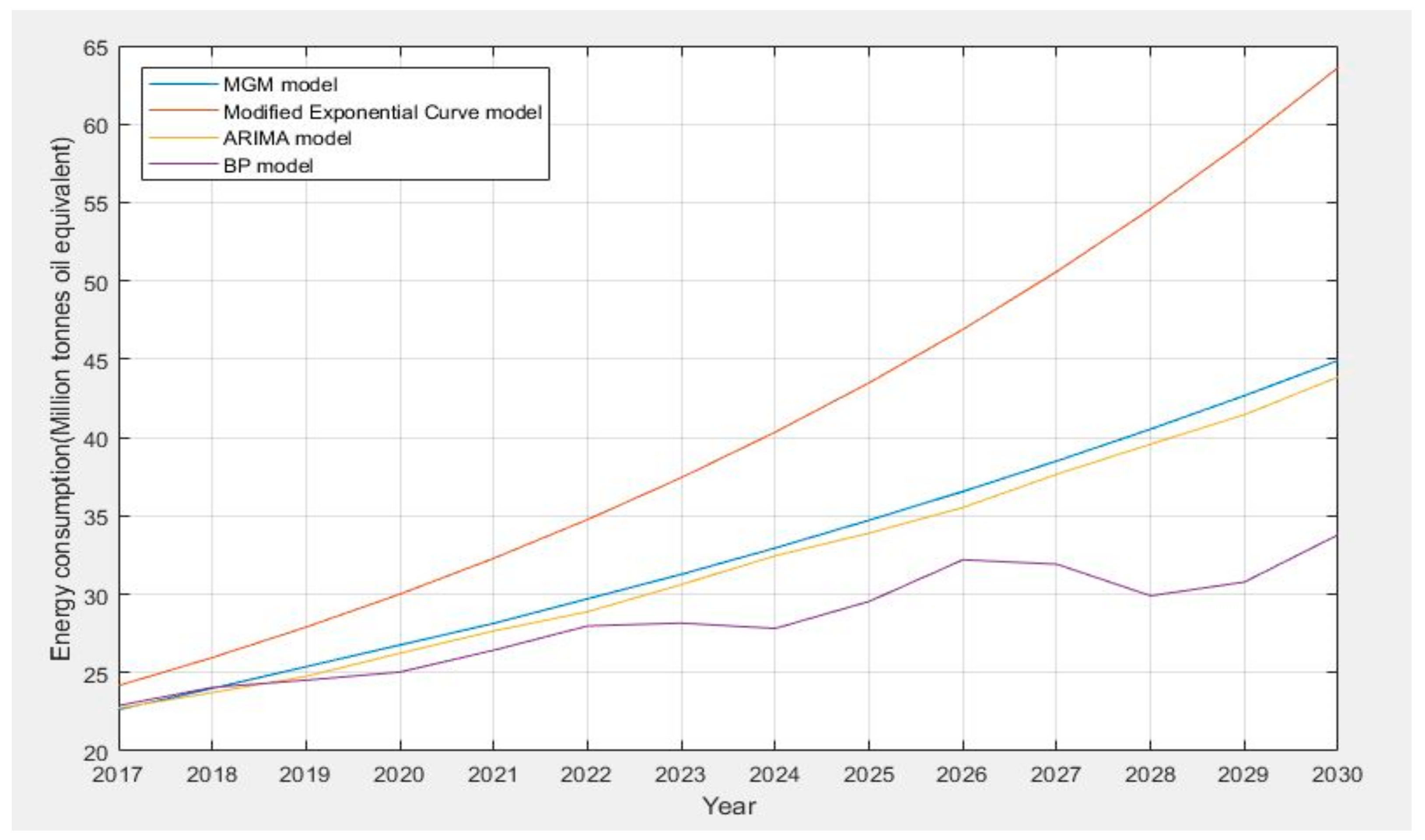
In this part, metabolic grey model (MGM), modified exponential curve method (MECM), autoregressive integrated moving average model (ARIMA), and BP neural network model (BP) are illustrated. Among those forecasting methods, a recent study shows that in the field of energy prediction, the top three most popular models are: Regression-based formulations, time series models and neural networks. We have established four models based on four theories: the grey theory, regression analysis theory, trend extrapolation theory, and neural network theory, and these theories cover both nonlinear and linear methods. The forecasting models used in the energy field are diverse. Each of them has their own strengths. Due to a common their feature, namely suitability for small sample prediction, four models that are totally different can be used to predict energy demand in the next 14 years in Middle Africa to provide four small sample prediction methods. Next, we will introduce the development of these four models separately.
Grey model was improved and applied by many scholars in many aspects, since Professor Deng, a famous Chinese scholar, founded the grey system theory in 1982 [20]. It is also widely used in energy forecasting field. Wu et al. established the grey model to forecast the energy supply in 2010–2020 in Shandong Province of China [21]. Kumar et al. developed a rolling grey model to forecast Indian crude oil consumption [22]. Improved grey model has higher prediction accuracy than traditional grey models [23]. In this paper, we put forward a metabolic grey model (MGM) to improve the accuracy by the rolling process. In the traditional grey model, only data from the previous four years are used to predict. The more backward the prediction data is, the less convincing the data will be. The MGM is based on the method of data substitution to improve the grey model. It uses five years data to predict the next year’s data, the latter will be pushed to the end. The continuously updated data can be fully utilized, and its accuracy can be greatly improved.
The modified exponential curve method (MECM) indicates that the development of the matter is exponential or near-exponential. Its application range is exponentially changing over a period of time, and the growth trend will slow down and stagnate as time goes by. This model is mostly used for the prediction of subgrade settlements. Zhou et al. used the Taylor expansion modified exponential curve method to predict subgrade settlement [24]. Its characteristics are consistent with the rapid development of Middle Africa, suggesting that the method can be applied to energy consumption predictions, in theory.
ARIMA model [25], can reflect the structure and characteristics of time series more essentially and then achieve the optimal prediction of minimum variance, which is different from the time series method that depends on different constraints [26,27]. This model has been widely used in public transport [28], health care [29] and other aspects of evaluation [30]. It is also used in the field of energy consumption. Bhutto et al. estimated gasoline consumption in the Pakistani transport sector in the past ten years by using the ARIMA method [31]. Wang et al. used a novel ARIMA model to forecast China’s dependency on foreign oil and it will exceed 80% by 2030 [32]. ARIMA model in energy prediction is potential.
BP neural network proposed by scientists led by Rumelhart and McClelland is a feedforward neural network implemented by a back-propagation algorithm [33], which is characterized by distributed storage and parallel cooperative processing of information, and its hidden layer can solve non-linear problems. Neural networks were usually used to find problems in electricity system configurations to prevent losses [34]. In addition, it can be used as an input for data generation for the scenario approach theory mentioned [35] for the case of energy system scheduling. BP neural network has great prospects in the field of energy prediction.
In terms of energy forecasting, previous scholars have put several methods together to predict. Yuan et al. used GM (1, 1) model and ARIMA model to predict China’s main energy consumption [36]. Cristina et al. presented ARIMA model and autoregressive neural network (NAR) model for energy consumption forecast [37]. Abdollah et al. proposed three forecasting models including autoregressive integrated moving average, the wavelet transform and artificial neural network, for short-term forecasting [38]. They used one, two [39] or even three models to predict energy problems, and this paper used four completely different types of predictive models. For comparison, it is difficult to find which model is more accurate, therefore we chose four models to forecast the same data.
The research on Middle Africa is rare, on the other hand, its resources play an important role in the world and its development should be of concern. Another reason is that the energy consumption data of Middle Africa used in this paper include three characteristics as follows:
(1)
Energy demand prediction only depends on single raw data.
(2)
The target of prediction is to show the energy demand in the next ten years, and these models can meet the need of long-term prediction.
(3)
It is limited data, belonging to a small sample.
According to these characteristics, we chose four models-improved GM, modified exponential curve, linear ARIMA and non-linear BP. Four models provide a multifaceted comparison and show the possibility of prediction from multi-angle. At last, a small sample study is the core of this paper, therefore we can get the ideal results by selecting an appropriate method to predict appropriate data. The method system we have established solved the limitations, further improved prediction accuracy, and provided a methodological reference.

3. Methods

3.1. MGM Model

The grey system theory is to establish the grey differential equation by extracting some known information, so as to realize the accurate description of the system’s operation law and make scientific prediction accordingly. The steps of MGM model are as follows:
Assume a raw sequence: X 0 = X 0 1 , X 0 2 , , X 0 N , accumulate X 0 to get a new first order differential equation: X 1 = X 1 1 , X 1 2 , , X 1 N , because it can weaken the randomness of raw data and make it present a more obvious characteristic law where, X 1 k = t = 1 k X 0 i , k = 1 , 2 , , n .
1-AGO sequence:
d X 1 d t + α X 1 t = μ
In the Equation (1), α and μ that are constant parameters can be calculated by the least square method by constructing accumulative matrix B and constant term vector Y N .
α μ = B T B 1 B T Y N
B = 1 2 X 1 1 + X 1 2 1 1 2 X 1 2 + X 1 3 1 1 2 X 1 N 1 + X 1 N 1
Y N = X 1 0 2 , X 1 0 3 , , X 1 0 N T
Bring the values of B and Y N into the calculation, and the predicted values can be got directly as follows:
X ^ 0 k + 1 = X ^ 0 k + 1 X ^ 0 k = 1 e α X 0 1 μ α e α k , k = 1 , 2 , , n

3.2. MECM Model

The modified exponential curve method is one of the trend extrapolation prediction methods in the time series model. The trend extrapolation prediction method includes an exponential curve, a modified exponential curve, a growth curve, and an envelope curve [40]. The staple steps of the modified exponential curve method are following.
Assume predictive value model:
y ^ = k + a b t
Divide the original observation value into three parts, each with m periods, and then make the sum of the trend values of each part equal to the sum of the corresponding observations, and thus the parameter can be calculated.
The sum of the original values of each part is as follows.
s 1 = t = 1 m y t , s 2 = t = m + 1 2 m y t , s 3 = t = 2 m + 1 3 m y t
s 1 = t = 1 m y t = t = 1 m ( k + a b t ) = m k + a b 1 + b + b 2 + + b m 1
s 2 = t = m + 1 2 m y t = t = m + 1 2 m ( k + a b t ) = m k + a b m + 1 1 + b + b 2 + + b m 1
s 3 = t = 2 m + 1 3 m y t = t = 2 m + 1 3 m ( k + a b t ) = m k + a b 2 m + 1 1 + b + b 2 + + b m 1
Because 1 + b + b 2 + + b m 1 b 1 = b m 1 ,
s 1 = m k + a b b m 1 b 1
s 2 = m k + a b m + 1 b m 1 b 1
s 3 = m k + a b 2 m + 1 b m 1 b 1
According to the above Equations (11)–(13), a and b , and k that are constant parameters can be calculated as follows.
b = s 3 s 2 s 2 s 1 1 m
a = s 2 s 1 b 1 b b m 1 2
k = 1 m s 1 a b b m 1 b 1

3.3. ARIMA Model

ARIMA (p, d, q) is a time series model that only needs endogenous variables rather than other exogenous variables. In fact, ARIMA model is the combination of differential operation and ARMA model that is made of autoregressive model (AR) and moving average model (MA) and because the fluctuation of any sequence can be regarded as a combination of deterministic and stochastic factors.
Raw sequence is Y t = y 1 0 , y 2 0 , , y m 0 , and the prediction sequence is Y t * = y 1 1 , y 2 1 , , y m 1 , where y m 0 means raw data and y m 1 means forecast data.
Autoregressive model (AR) describes the history and current value of the relationship between the model, it is itself the variable historical event data to predict its own way. The equation is following:
Y t * = c + γ 1 Y t 1 + γ 2 Y t 2 + + γ p Y t p + μ t
The moving average model (MA) focuses on the autoregressive model error accumulation. It can effectively eliminate the random fluctuations in the prediction. The equation is as follows:
Y t * = μ t + β 1 μ t 1 + β 2 μ t 2 + + β q μ t q
By combining the AR model with the MA model, the ARMA model can be obtained. The equation is as follows:
Y t * = c + γ 1 Y t 1 + γ 2 Y t 2 + + γ p Y t p + μ t + β 1 μ t 1 + β 2 μ t 2 + + β q μ t q
The predicted values can be expressed as: Y t * = 1 B d Y t , where, B = y 1 1 + y 2 1 2 1 y m 1 1 + y m 1 2 1

3.4. BP Neural Network

BP neural network simulates human brain nerve processing information through a large number of simple neurons interconnected and carries out parallel processing and non-linear transformation of information [41]. Figure 1 shows the structure of BP neural network.
In the structure of BP Neural Network, there are i input values, j hidden layers and k output values. The connection weight is w i j and T j k . The essence of BP neural network is to transform a group of input and output samples into a non-linear optimization problem, and to solve the weight problem by using iterative operation. The input layer receives data and the output layer outputs data. The next layer of neurons collects the information from the previous layer of neurons and passes the value to the next layer after “activation”. In this model, the activation function is sigmoid z = 1 1 + e z , which leads to the introduction of nonlinearity in the model [42]. Similarly, when extended to multiple neuron combinations, it is possible to better fit nonlinear data by continuous learning. Adding an activation function is used to add nonlinear factors and solve problems that cannot be solved by linear models.
Its main learning process is divided into two parts. The first part is the process of information forward propagation. In the forward propagation, the input information is processed by the input and hidden layers and passed on the output layer. The formula for determining the hidden layer is as follows: y i = f ( j w i j θ i ) , j = 1 , 2 , , l , where θ i means node threshold. The output layer formula is determined as follows: O i = f ( j T i j θ i ) , j = 1 , 2 , , l .
If the output layer is unable to obtain the required output, it enters the second part that is the error back-propagation process. It is along the original path return error signal and achieves the desired output by repeatedly modifying the weights and thresholds.

4. Empirical Results and Discussion

The operation process of several models will include the calculation process and accuracy analysis. In this section, the forecast of existing data is used as a fitting process. In other words, by forecasting energy demand in Middle Africa to compare with the existing data from 1994 to 2017, a total of 24 years of data, the fitting degree of the four models can be measured and established. And then we will use four models to predict the energy demand in Middle Africa in the next 14 years, until 2030.
The data of energy consumption is selected from “BP Statistical Review of World Energy”. The raw data on energy consumption in Middle Africa and its annual growth rate are shown in Figure 2. The overall trend is upward. In 1994, 1997, and 1998, the growth rate was negative. At the beginning of the 21st century, the growth rate was positive and relatively stable, except for a significant increase in 2006.

4.1. MGM Parameters

Using this set of data, we will establish the prediction of MGM model, the linear regression model forecasts future data according to the linear time series, and the 1-AGO sequence has sharper linear characteristics. Figure 3 shows the first-order cumulative sequence of the raw data, which more obviously illustrates the linear characteristic than the original sequence. Thus, the MGM model is used to predict the 1-AGO sequence.
This 1-AGO sequence is inputted into the MGM model. Since the fifth data, the rolling process of MGM generates a set of parameter values for each data. In other words, since the fifth set of data, when five consecutive values of the input sequence enter MGM model, the sixth prediction value is generated. In each iteration, a differential equation is established, in which ‘ α ’ and ‘ μ ’ are the operational coefficients of the MGM model. Parameter ‘ α ’ and ‘ μ ’ can be calculated by matrix operation and least squares. Figure 4 shows the value of α and μ and Table A2 (Appendix A) shows specific values.
On the basis of this parameter table, the prediction sequence of MGM model, that is called the fitting sequence, can be obtained.

4.2. MECM Parameters

The modified exponential curve method requires that the data be divided into three groups. In this paper, the data used is the energy consumption data of Middle Africa from 1994 to 2017, a total of 24 sets of data. The data are divided into three groups of eight sets of data each. Then, the three sets of data are respectively summed according to Equation (9).
Using Matlab software to program according to the calculation process of the modified exponential curve method, we calculated b = 1.0834 , a = 3.1525 , k = 2.6265 . Therefore, the model established by the modified exponential curve method is y ^ = 2.6265 + 3.1525 × 1.0834 t .
According to the above Equations (14)–(16), the predicted values and residuals predicted by MECM model are shown in Table 1.

4.3. ARIMA Parameters

The ARIMA model predicts the stationary sequence. The original series is nonstationary, therefore, we use differential tools to smooth the sequence.
The results of the unit root test in Table 2 show the original residual sequence is nearly stationary under the condition of second-order difference processing. The difference number (d) is determined to be two by unit root test. On this basis, if the coefficient enter diagram slowly tends to zero, it is classified as trailing. On the contrary, if the coefficient graph suddenly tends to zero, it means truncation. The judgment of tail and truncation supports the determination of coefficients ‘p’ and ‘q’, which can be obtained in correlation coefficient diagram of stationary residual sequence (Figure 5) with the help of EViews 7.2.
Different parameters have different accuracy. After continuous simulation with SPSS Statistics v. 22 software (IBM, Armonk, NY, USA), ARIMA (6, 2, 6) model is selected to predict the residual sequence. In order to determine the goodness of fitting ARIMA model, we select the R-square value to evaluate the model, where the greater the stationary R square value, the higher the accuracy of the corresponding model. When the value of p is six and the value of q is six, the R-square value is 0.628 > 0.6, which shows that the fitting effect is good.

4.4. BP Neural Network Parameters

We use Matlab to build BP neural network, because the neural network box of MATLAB provides convenience for BP network modeling [43]. Firstly, an initialization network model is established. The single hidden layer network structure is used to control the fitting process [44]. In order to ensure the accuracy of the model and improve the prediction accuracy, we add a loop statement. After many experiments, the number of input layer nodes, output layer nodes, and hidden layer nodes is determined to be 4, 1 and 10 respectively. Figure 6 shows the structure of the BP model.
And then the network training stage includes two steps:
Forward propagation: The original value is used as input data, and the sample is passed into the hidden layer, then output through the output layer through the activation function.
Back-propagation: If the output value does not satisfy the requirement, the weight is adjusted. When the error changes from decreasing to rising, the network stops training.
Finally, using the “sim” function to achieve the simulation z = sim net , pr , where z represents the output data, net represents the object of the neural network, and pr represents the input vector. In this process, the original value is used as an input sample.

4.5. Evaluation and Comparison of Four Models

Next, the forecast performance of MGM model and MECM model, ARIMA model, and BP model will be illustrated. Figure 7 shows the fitting data of four models with the raw data and the concrete fitting data can be found in Table A1 (Appendix A). The green line represents the raw data from 1994 to 2017, and the remaining lines are the fitting values of the four models.
It can be seen from the graph that there is little difference between the fitting values and the original values of the four models, which shows that the prediction results of the four models used in this paper are also convincing.
In order to describe the prediction performance of the models more accurately, we can use fitting data to calculate the accurate error value in this part. Root mean square error (RMSE) and Mean absolute percent error (MAPE) are chosen and the equations are as follows. The precise results are shown in Table 3.
RMSE = 1 n i = 1 n y i x i 2
MAPE = 1 n i = 1 n y i x i x i
where ‘ n ’, ‘ y i ’, ‘ x i ’ are sample size, fitting value and truth value, respectively.
By comparing the data, we can see that BP model has the highest accuracy, followed by the ARIMA model, the MGM model, and the MECM model. The MAPE values of the four modes are under 5%, which proves that the accuracy of these models is high, the prediction results are trustworthy.
In addition, based on the relative error values, we can see the reliability of these models. The following is the equation:
Goodness = 1 P r e d i t i o n M e t a d a t a M e t a d a t a
Figure 8 shows the prediction accuracy of the four models per year. Although the accuracy of every year is different, it can be seen that the average accuracy of the four models is around 90%, which further shows the reliability of these four models is very good.

4.6. Forecast Results

According to the energy consumption data of 1994–2016 obtained by BP World Energy Statistics Review 2018, Figure 9 shows the results of the future 14 years prediction of energy demand for Middle Africa by the four models and the specific data can be seen in Table A3 (Appendix A). Although the forecast results of the four models are slightly different, the basic trend is the same. Energy demand in Middle Africa will increase in the future.
The forecast results show that the growth rates of energy demand from 2017 to 2030 in Middle Africa are 5.41%, 7.73%, 5.19%, and 3.13% respectively according to MGM model, MECM model, ARIMA model and BP model.

5. Conclusions

In this paper, comparing four completely different types of predictive models can help to fully describe the characteristics of the predictive data and provide a multi-angle analysis of the predicted results by taking Middle Africa as an example. The MGM model, MECM model, ARIMA model, and BP model are used to predict energy demand in Middle Africa until 2030. The MAPE of four models are 2.41%, 4.80%, 1.91%, and 0.88%, respectively. These methods will be valuable for future related research. The forecast results show that energy consumption in Middle Africa will grow at a rate of about 5.37% over the next 14 years. Energy demand in Middle Africa will continue to grow, which indicates that Middle Africa has great potential for economic development.
However, the time vector is used as the only input parameter in this paper. Although the accuracy of BP prediction results is the highest, the conditions are often complex. Therefore, the application of BP neural network in energy forecasting still needs further exploration.

Author Contributions

L.W. conceived and designed the experiments, wrote the original paper; R.L. performed the experiments, and analyzed the data; L.Z. contributed analysis tools and revised the original paper. All authors read and approved the final manuscript.

Funding

Current work is supported by the Recruitment Talent Fund of China University of Petroleum (East China) (YJ2016002). We have received the grants in support of our research work.

Conflicts of Interest

The authors declare no conflict of interest.

Appendix A

Table A1. Middle Africa’s fitting results of four models (million tonnes oil equivalent).
YearRaw DataMGMGoodness of MGMMECMGoodness of MECMARIMAGoodness of ARIMABPGoodness of BP
19946.84296.8429100.00%6.041888.29%6.8429100.00%6.8429100.00%
19957.02437.090099.07%6.326590.07%7.0243100.00%7.0243100.00%
19967.06667.019499.33%6.634993.89%7.220097.83%7.0666100.00%
19977.05296.949698.54%6.969198.81%7.210097.77%7.0529100.00%
19986.79356.880498.72%7.331092.09%7.200094.02%6.7935100.00%
19997.09456.812096.02%7.723291.14%6.890097.12%5.988884.42%
20007.71706.958990.18%8.148194.41%7.100092.00%7.7170100.00%
20018.19117.770394.86%8.608494.91%7.930096.81%8.1911100.00%
20028.57028.734898.08%9.107093.74%8.730098.14%8.5702100.00%
20039.22279.185999.60%9.647295.40%9.160099.32%9.2227100.00%
200410.07529.722896.50%10.232598.44%9.490094.19%10.0752100.00%
200510.248510.715695.44%10.866593.97%10.460097.94%10.2485100.00%
200611.647011.072295.06%11.553499.20%11.420098.05%11.6470100.00%
200712.603512.311297.68%12.297697.57%12.790098.52%12.6035100.00%
200813.724013.596999.07%13.103795.48%13.660099.53%13.7240100.00%
200914.693915.145396.93%13.977195.12%14.700099.96%14.6939100.00%
201015.934415.922599.93%14.923393.65%16.100098.96%15.9344100.00%
201116.790217.186497.64%15.948494.99%16.900099.35%16.643399.12%
201217.373918.061396.04%17.058998.19%17.630098.53%17.840397.32%
201318.525318.516899.95%18.261998.58%18.620099.49%18.5253100.00%
201419.782119.356197.85%19.565398.90%19.700099.58%19.485698.50%
201520.487820.809898.43%20.977397.61%20.730098.82%20.4878100.00%
201621.552421.825998.73%22.507195.57%21.720099.22%21.571799.91%
201722.960322.643198.62%24.164394.76%22.730099.00%22.895699.72%
Table A2. The values of parameters α and μ of the MGM model.
Year1999200020012002200320042005
α 0.010.0025−0.0328−0.0649−0.0617−0.0583−0.0706
μ 7.19397.05526.4726.06376.53867.06457.2526
Year2006200720082009201020112012
α −0.0611−0.073−0.0816−0.0938−0.0778−0.077−0.0681
μ 7.90888.23658.6638.981610.419111.253712.4333
Year2013201420152016
α −0.0544−0.0489−0.0563−0.0554
μ 13.747714.812815.253216.0776
Table A3. Prediction results for the next fourteen years with four models.
YearMGM MECM ARIMA BP
201823.99085.95%25.95977.43%23.73004.40%24.05395.06%
201925.37845.78%27.90477.49%24.76004.34%24.51871.93%
202026.76495.46%30.01197.55%26.24005.98%25.03542.11%
202128.14505.16%32.29477.61%27.66005.41%26.42965.57%
202229.71175.57%34.76797.66%28.89004.45%27.97835.86%
202331.27695.27%37.44727.71%30.62005.99%28.16060.65%
202432.95305.36%40.34987.75%32.46006.01%27.8203−1.21%
202534.72585.38%43.49447.79%33.90004.44%29.54356.19%
202636.56015.28%46.90127.83%35.54004.84%32.20018.99%
202738.50335.32%50.59197.87%37.66005.97%31.9195−0.87%
202840.53865.29%54.59037.90%39.58005.10%29.9038−6.31%
202942.67515.27%58.92197.93%41.46004.75%30.78262.94%
203044.91705.25%63.61477.96%43.87005.81%33.80419.82%

References

  1. Oladiran, M.T.; Meyer, J.P. Energy and exergy analyses of energy consumptions in the industrial sector in South Africa. Appl. Energy 2007, 84, 1056–1067. [Google Scholar] [CrossRef]
  2. Suganthi, L.; Samuel, A.A. Energy models for demand forecasting—A review. Renew. Sustain. Energy Rev. 2012, 16, 1223–1240. [Google Scholar] [CrossRef]
  3. Wei, L. Brief Analysis of Energy Development in Africa. China’s Collect. Econ. 2010, 25, 199–200. [Google Scholar]
  4. Kebede, E.; Kagochi, J.; Jolly, C.M. Energy consumption and economic development in Sub−Sahara Africa. Energy Econ. 2010, 32, 532–537. [Google Scholar] [CrossRef]
  5. Mohammed, Y.S.; Mustafa, M.W.; Bashir, N. Status of renewable energy consumption and developmental challenges in Sub–Sahara Africa. Renew. Sustain. Energy Rev. 2013, 27, 453–463. [Google Scholar] [CrossRef]
  6. Szabó, S.; Bódis, K.; Huld, T.; Moner-Girona, M. Sustainable energy planning: Leapfrogging the energy poverty gap in Africa. Renew. Sustain. Energy Rev. 2013, 28, 500–509. [Google Scholar]
  7. Wang, Q.; Chen, X. Energy policies for managing China’s carbon emission. Renew. Sustain. Energy Rev. 2015, 50, 470–479. [Google Scholar] [CrossRef]
  8. Lin, B.; Wesseh, P.K. Energy consumption and economic growth in South Africa reexamined: A nonparametric testing apporach. Renew. Sustain. Energy Rev. 2014, 40, 840–850. [Google Scholar] [CrossRef]
  9. Wang, Q. Effective policies for renewable energy—the example of China’s wind power—lessons for China’s photovoltaic power. Renew. Sustain. Energy Rev. 2010, 14, 702–712. [Google Scholar] [CrossRef]
  10. Wang, Q.; Li, R. Drivers for energy consumption: A comparative analysis of China and India. Renew. Sustain. Energy Rev. 2016, 62, 954–962. [Google Scholar] [CrossRef]
  11. British Petroleum. Statistical Review of World Energy; British Petroleum: London, UK, 2017. [Google Scholar]
  12. Landman, W.A.; Goddard, L. Statistical Recalibration of GCM Forecasts over Southern Africa Using Model Output Statistics. J. Clim. 2001, 15, 2038–2055. [Google Scholar] [CrossRef]
  13. Landman, W.A.; Beraki, A. Multi–model forecast skill for mid–summer rainfall over southern Africa. Int. J. Climatol. 2012, 32, 303–314. [Google Scholar] [CrossRef]
  14. Collins, D.C.; Reason, C.J.; Hewitson, B. An analysis of the output of the Hadley Centre Unified Model forecast for Southern Africa using Nonlinear Primary Component Analysis (NLPCA) for feature recognition. In Proceedings of the Agu Spring Meeting, Boston, MA, USA, 1 May 2001. [Google Scholar]
  15. Singh, A.; Kumar, S.; George, J.P. Dust forecast over North Africa: Verification with satellite- and ground-based observations. In Proceedings of the Remote Sensing of the Atmosphere, Clouds, & Precipitation VI, New Delhi, India, 9 May 2016. [Google Scholar]
  16. Darwish, A.S.; Shaaban, S. Solar and Wind Energy–Present and Future Energy Prospects in the Middle East and North Africa; Sayigh, A., Ed.; Springer: Cham, Switzerland, 2015. [Google Scholar]
  17. Jebli, M.B.; Youssef, S.B. The role of renewable energy and agriculture in reducing CO2 emissions: Evidence for North Africa countries. Ecol. Indic. 2017, 74, 295–301. [Google Scholar] [CrossRef]
  18. Ramanathan, R. An analysis of energy consumption and carbon dioxide emissions in countries of the Middle East and North Africa. Energy 2005, 30, 2831–2842. [Google Scholar] [CrossRef]
  19. Inglesi, R. Aggregate electricity demand in South Africa: Conditional forecasts to 2030. Appl. Energy 2010, 87, 197–204. [Google Scholar] [CrossRef]
  20. Deng, J. Grey System Fundamental Method; Huazhong University of Science and Technology: Wuhan, China, 1982. [Google Scholar]
  21. Wu, S.J.; Wu, X.J.; Liu, X.M. GM (1, 1) Grey Forecasting and Analysis on Energy Production and Supply in Shandong Province. In Proceedings of the International Conference on Management & Service Science, Wuhan, China, 12 August 2011. [Google Scholar]
  22. Kumar, U.; Jain, V.K. Time series models (Grey–Markov, Grey Model with rolling mechanism and singular spectrum analysis) to forecast energy consumption in India. Energy 2010, 35, 1709–1716. [Google Scholar] [CrossRef]
  23. Wang, Q.; Li, S.; Li, R. Forecasting energy demand in China and India: Using single–linear, hybrid–linear, and non–linear time series forecast techniques. Energy 2018, 161, 821–831. [Google Scholar] [CrossRef]
  24. Chun-Hui, S.U.; Zhou, J.; Pan, H.Z. The Applied Analysis on Taylor Expansion Modified Exponential Curve Method for Subgrade Settlement Prediction; Construction & Design for Project: Changsha, China, 2013. [Google Scholar]
  25. Wang, Q.; Song, X.; Li, R. A novel hybridization of nonlinear grey model and linear ARIMA residual correction for forecasting U.S. shale oil production. Energy 2018, 165, 1320–1331. [Google Scholar] [CrossRef]
  26. Muriana, C.; Tommaso, P.; Giovanni, V. An expert system for financial performance assessment of health care structures based on fuzzy sets and KPIs. Knowl. Based Syst. 2016, 97, 1–10. [Google Scholar] [CrossRef]
  27. Aiello, G.; Cannizzaro, L.; La Scalia, G.; Muriana, C. An expert system for vineyard management based upon ubiquitous network technologies. Int. J. Serv. Oper. Inform. 2011, 6, 230–247. [Google Scholar] [CrossRef]
  28. Liu, J.H. Application of ARIMA model in predicting the incidence of HFMD in Yichang city. China Trop. Med. 2014, 14, 956–958. [Google Scholar]
  29. Yue-Hua, H.U. Application of multiple seasonal autoregressive integrated moving average model in prediction of incidence of hand foot and mouth disease in China. Dis. Surveill. 2014, 64, 1801–1808. [Google Scholar]
  30. Wang, Q.; Li, S.; Li, R.; Ma, M. Forecasting U.S. shale gas monthly production using a hybrid ARIMA and metabolic nonlinear grey model. Energy 2018, 160, 378–387. [Google Scholar] [CrossRef]
  31. Bhutto, A.W.; Bazmi, A.A.; Qureshi, K.; Harijan, K.; Karim, S.; Ahmad, M.S. Forecasting the consumption of gasoline in transport sector in pakistan based on ARIMA model. Environ. Prog. Sustain. Energy 2017, 36, 1490–1497. [Google Scholar] [CrossRef]
  32. Wang, Q.; Li, S.; Li, R. China’s dependency on foreign oil will exceed 80% by 2030: Developing a novel NMGM–ARIMA to forecast China’s foreign oil dependence from two dimensions. Energy 2018, 163, 151–167. [Google Scholar] [CrossRef]
  33. Wang, L.; Wang, A.; Qu, H.; Liu, S. Optimal Forecast Combination Based on Neural Networks for Time Series Forecasting. Appl. Soft Comput. 2018, 66, 1–17. [Google Scholar] [CrossRef]
  34. Modarresi, M.S.; Huang, T.; Ming, H.; Xie, L. Robust Phase Detection in Distribution Systems. In Proceedings of the 2017 IEEE Texas Power and Energy Conference (TPEC), College Station, TX, USA, 9 February 2018. [Google Scholar]
  35. Modarresi, M.S.; Xie, L.; Campi, M.; Garatti, S.; Carè, A.; Thatte, A.; Kumar, P.R. Scenario−Based Economic Dispatch with Tunable Risk Levels in High−renewable Power Systems. In Proceedings of the IEEE Transactions on Power System, College Station, TX, USA, 18 October 2018. [Google Scholar]
  36. Yuan, C.; Liu, S.; Fang, Z. Comparison of China’s primary energy consumption forecasting by using ARIMA (the autoregressive integrated moving average) model and GM(1,1) model. Energy 2016, 100, 384–390. [Google Scholar] [CrossRef]
  37. Nichiforov, C.; Stamatescu, L.; Făgărăşan, L.; Stamatescu, G. Energy consumption forecasting using ARIMA and neural network models. In Proceedings of the International Symposium on Electrical & Electronics Engineering, Galati, Romania, 20–22 October 2017. [Google Scholar]
  38. Akbari-Zadeh, M.R. A hybrid method based on wavelet, ANN and ARIMA model for short-term load forecasting. J. Exp. Theor. Artif. Intell. 2014, 26, 167–182. [Google Scholar]
  39. Wang, Q.; Li, S.; Li, R. Will Trump’s coal revival plan work?—Comparison of results based on the optimal combined forecasting technique and an extended IPAT forecasting technique. Energy 2019, 169, 762–775. [Google Scholar] [CrossRef]
  40. Mengxue, S. Application of Modified Exponential Curve Method in Settlement Prediction of Soft Soil Subgrade. Transp. Technol. 2014, 21, 61–64. [Google Scholar]
  41. Wei, W.; Qiang, C.W.; Liu, P. Prediction of Stock Market Rise and Drop by BP Neural Network. J. Dalian Univ. Technol. 2001, 41, 9–15. [Google Scholar]
  42. Shi, L.; Liu, S.; Yan, G.; Mu, H. Temperature prediction of the molten salt collector tube using BP neural network. Renew. Power Gener. IET 2016, 10, 212–220. [Google Scholar]
  43. Sadeghi, B.H.M. A BP-neural network predictor model for plastic injection molding process. J. Mater. Process. Technol. 2000, 103, 411–416. [Google Scholar] [CrossRef]
  44. Wang, S.; Zhang, N.; Wang, Y.; Wu, L. Wind speed forecasting based on the hybrid ensemble empirical mode decomposition and GA–BP neural network method. Renew. Energy 2016, 94, 629–636. [Google Scholar] [CrossRef]
Figure 1. The structure of Three-Layer BP Neural Network.
Sustainability 11 02436 g001
Figure 2. Energy consumption and its growth rate of Middle Africa in 1994–2017.
Sustainability 11 02436 g002
Figure 3. 1-AGO sequence of Middle Africa (million tonnes oil equivalent).
Sustainability 11 02436 g003
Figure 4. The value of parameters of metabolic grey model (MGM) model.
Sustainability 11 02436 g004
Figure 5. Correlation coefficient diagram of stationary residual sequence.
Sustainability 11 02436 g005
Figure 6. The structure of BP neural network model in MATLAB.
Sustainability 11 02436 g006
Figure 7. Comparison of four models (MGM model, MECM model, autoregressive integrated moving average model (ARIMA) model, BP model) between fitting and raw data.
Sustainability 11 02436 g007
Figure 8. Goodness-of-fit values of multiple models at different time points.
Sustainability 11 02436 g008
Figure 9. Forecast the energy demand of Middle Africa with four models (million tonnes oil equivalent).
Sustainability 11 02436 g009
Table 1. The predicted values and residuals of the modified exponential curve method (MECM) model (million tonnes oil equivalent).
tRaw DataPredicted Values of MECMResiduals
16.84296.0418−0.8012
27.02436.3265−0.6979
37.06666.6349−0.4317
47.05296.9691−0.0838
56.79357.33100.5376
67.09457.72320.6287
77.71708.14810.4311
88.19118.60840.4172
98.57029.10700.5368
109.22279.64720.4246
1110.075210.23250.1573
1210.248510.86650.6180
1311.647011.5534−0.0936
1412.603512.2976−0.3060
1513.724013.1037−0.6203
1614.693913.9771−0.7168
1715.934414.9233−1.0111
1816.790215.9484−0.8419
1917.373917.0589−0.3150
2018.525318.2619−0.2633
2119.782119.5653−0.2168
2220.487820.97730.4895
2321.552422.50710.9546
2422.960324.16431.2040
Table 2. Middle Africa difference results and unit root test based on EViews 7.2.
SequenceADF StatisticCritical ValueValue of p
1%5%10%
Q4.3759823.7529462.9980642.6387520.0000
Q *−2.1958913.8315113.0299702.6551940.0000
Q **−5.0332663.8315113.0299702.6551940.0000
Note: Q means zero order difference; Q * means first order difference; Q ** means second order difference.
Table 3. Error values of multiple models.
MGMMECMARIMABP
RMSE35.08%60.52%24.76%25.45%
MAPE2.41%4.80%1.91%0.88%

