Decomposing the Driving Factors of Water Use in China

Abstract

Based on the national input–output table, a comparable price non-competitive input–output table was compiled for 2002, 2007, and 2012. The influence factors of price and product imports were removed from the table. Furthermore, a water-use input–output table was constructed based on the links between the economic system and water resources management. With the multi-factor structural decomposition analysis (SDA) model developed in this paper, the driving forces of water use were decomposed into 18 factors, and quantitative effect results were obtained. Total water use in China increased by 3.9% from 2002 to 2007 and by 5.4% from 2007 to 2012 with the combined effects of multiple factors. For example, the increase in economic scale raised water use by 46.6% and 45.5%, respectively. Advancement in agricultural technology (production and water-saving technologies) reduced water use by 14.9% and 19.8%, respectively. Reducing the proportion of thermal/nuclear power and increasing the price of electricity have water use-reducing effects. Changes in the mode of development considerably reduced water use by 9.5% and 5.3%, respectively. Water-use management should focus on factors that have great influence on water use and show high water-use sensitivity.

1. Introduction

China’s per capita water resource amounts to 2100 m³ (2012), which is lower than the world average. As one of the 13 most water-poor countries in the world, water shortage would critically hinder China’s sustainable development [1]. Water resources are a core element for both grain and energy security. From 2002 to 2015, irrigation water accounted for approximately 55% of total water use, while thermal and nuclear power generation accounted for around 8% of total water use [2,3]. Along with rapid economic development, the demand for grain and electricity is also growing swiftly, creating new challenges for the management of the already severe water shortage problem. To cope with this shortage and improve water-use efficiency, the government has adopted a series of water-saving policies and measures, including investments in farmland water conservancy facilities and implementation of water-saving technology reforms in the power, steel, petrochemical, and other industries. In addition, social and economic measures (e.g., industrial restructuring and transformation of economic development modes) have also reduced water use [4]. Overall, total water use has fluctuated around 610 billion m³ (2011–2015), and has not increased in accordance with China’s economic aggregates.

Total water use seems to have decoupled from economic and social development. This trend is the result of various factors acting in tandem. To study the dynamic relationship between water resources and economic development, we must decompose these driving factors, and then quantitatively analyze each factor’s “force” on China’s water use. This will also be beneficial to research on national water use trend analysis and water resource carrying capacity, and has practical significance for effectively coping with water shortages.

Thus far, most research on the factors that drive water use has been qualitative or conceptual, resulting in a lack of effective quantitative research. Structural decomposition analysis (SDA) models based on input–output tables are widely used in research on economics, grains, energy, the environment, and other areas [5,6,7,8,9]. Moreover, there has been an increase in the use of this method in water resource and wastewater research [10,11,12]. Rose and Chen [13] argue that the essence of SDA is the use of key parameters in the input–output table for comparative static analysis of economic system changes. Cazcarro et al. [14] used SDA to analyze the impact factors of Spanish water use, including technology, input substitution, and final demand changes, from 1980 to 2007. Improvement in water technology and efficiency in Spain and changes in agricultural cultivation have produced important water-reducing effects. Yang et al. [15] studied the changes in China’s water use across various industries between 1997 and 2007. They analyzed the influence of water-saving technology level, economic system efficiency, population size, consumption level, and final demand structure on changes in water use. Li et al. [16] analyzed how water-saving technology level, intermediate technology level, final demand scale, final demand structure, and industry structure drove the evolution of water use in China.

Although these studies can be considered quantitative, their identification of driving factors was relatively limited, leading to the following problems. First, the influence of water-saving technology level and economic scale may have been exaggerated. These influences cancel each other out, such that the water use increase driven by economic development is offset by advancements in water-saving technology. Thus, the significance of the quantitative research is weakened. Second, characterizing a complex economic system using too few factors is inevitably problematic. This ignores the complex systemic nature of the water resources–economy dynamic, such as the water-reducing effect in electricity and grain production or the impact of changes in the economic development mode.

This study used the national input–output table [17,18,19] to compile a water-comparable non-competitive input–output table for 2002, 2007, and 2012. An SDA was performed to reveal the relationship between water use and the socio-economic system. To analyze the effects of the socio-economic system on water use, the determinants of water use were divided into 18 driving factors. Importantly, China still faces a water crisis due to the increase in water consumption and water pollution. Therefore, choosing to study the effect of economic system on water consumption has greater significance. The remainder of this paper is structured as follows. Section 2 describes how economic factors drive the evolution of water use in agricultural and industrial production, the services, and the domestic sector. Section 3 introduces the preparation process of the input–output table and the decomposing model methods. Section 4 analyzes the results and the main driving factors. Finally, the conclusions are summarized in Section 5.

2. Economic Factors Drive the Evolution of Water Use

In this study, total water use refers to the gross water volume used by all types of water users, including water loss but excluding ecological and environmental water use. Total water use refers to the flow of water from natural systems to economic and social systems used as a resource. The internal reuse of water in industrial and agricultural production processes and the utilization of seawater during the cooling process are not included.

In agricultural production, rainfed agriculture is on the decrease because its output is limited by natural conditions. Production is more stable with irrigated agriculture due to artificial irrigation. The Water Resources Bulletin [2,20,21] divides agricultural water use into water for crop farming, forestry, animal husbandry, and fisheries. Among these, water for crop farming accounts for the biggest proportion of agricultural water use. Considering the output value of one unit, water use for crop farming is also higher than that for forestry, animal husbandry, or fisheries. Thus, the proportion of crop farming, the proportion of irrigated agriculture, irrigation water efficiency, and the output capacity of agriculture affect agricultural water use at the same time.

In industrial production, thermal/nuclear power production and supply require a large amount of water for cooling. Thus, it is necessary to independently analyze this type of water use. The proportion of thermal and nuclear power in total power generation, the water use per unit power generation, and the output value of power industry has combined effects on water use in industry [22]. Water used in other industrial production processes includes vapor circulating water, cooling water, hydraulic de-dusting and slagging water, heating water, lavation water, desulfurization water, desalination water, raw material water, and so forth. Enterprises can reduce the use of fresh water by investing in water-saving equipment, water-recycling equipment, and alternative water equipment, for example. We may consider these to be “water-saving technological advancements.” In addition, we may also consider the water-reducing effect from reduced use of intermediate inputs in production processes to be “production technological advancements.”

The service industry can usually be divided into productive, consumer, and public services. Its output value of one unit water resource is very high, and the water used is mostly from centralized water supplies. Because of technological advancements, the efficiency of water use has improved continuously. Domestic water use is linked to the water supply facilities, resident consumption level, seasons, water prices, and so on [23]. With the improvements in consumption level and water supply facilities, the demand for water has become diverse, leading to an increase in per capita water use. The increasing application of water-saving facilities leads to a decrease in per capita water use.

Since water is used throughout the production and consumption process, it is important to deconstruct the driving forces of various factors on water use from the economic system. Gross domestic product (GDP), which is used as an indicator to characterize both the economic system and the changes in industrial structures, has an impact on water use. Generally, an increase in economic scale will increase total water use. Consumption, investment, and exports are the “motive power” of economic development, and changes in the structure among these three have an impact on water use. Imported products and services have a certain substitution effect on local products and services. An increase in imports can reduce the production of local intermediate products and services, and thus reduce consumption of domestic water resources. The effect on water use from the evolution of industrial structures depends on the proportion of water-intensive industries.

3. Materials and Methods

3.1. Water Input–Output Model

The complexity of quantitative research on the economic driving factors of water evolution is related to the complexity of the economic system. As the input–output table is the basis for national economic accounting, it can be used to study the “force” of different driving factors after appropriate expansion.

Table 1. The water non-competitive (import) input–output model.

Input/Output	Intermediate Input	Final Demand (Consumption, Fixed Assets, and Exports)	Import	Total Output
Domestic product	$A^{i}X$	$Y^i$		$X={\left(I-A\right)}^{-1}Y=LY$
Imported product	$A^{e}X$	$Y^e$	P
Added value	V
Total input	$X^T$
Water use	$W_1$	$W_2$		W

is the simplified water-comparable non-competitive input–output table used in this study. The intermediate input and output consist of all the departments in the society.

The basic equation of the input–output model is:

$$X=I-A^{-1}Y=LY$$

(1)

X is the total output matrix, I is a unit matrix, A is the total technical coefficient matrix, and Y is the final demand matrix, consisting of consumption, fixed assets, and exports. L is the Leontief inverse matrix that is other departments’ consumption by each department’s final consumption. L reflects the production technology, that is, the industry’s consumption of intermediate products and its output efficiency. V is the total added value matrix. P is the total import product value matrix. The superscript i denotes domestic products, and superscript e indicates imported products.

Water-use data are linked to this input–output table, where:

$$W=W_1+W_2$$

(2)

W is total water use, $W_1$ is the industry production water-use matrix, and $W_2$ is domestic water use. The water use data were obtained from the Water Resources Bulletin [2,21], which does not classify water use into specific departments. Thus, water use needs to be decomposed into industry departments.

The agricultural water-use data were sourced directly from the Water Resources Bulletin, and the data for the power production and the supply industry were obtained from the thermal and nuclear power water-use data in the Water Resources Bulletin [2,20,21]. For the other industries, the intermediate input proportion in each industry was divided according to the “water production and supply industry” in the input–output table. Li et al. [16] considered this method relatively more reliable after validating it with the economic census data. In the Water Resources Bulletin [2,20,21], urban domestic water use includes the construction industry, service industry, and urban domestic water uses. The construction and urban domestic water-use data were decomposed according to national water census data [24]. Finally, service industry water use was obtained by multiplying the portion used for final consumption in each service industry by the total water use in the service industry according to the water production and supply industries data in the input–output table.

3.2. Compilation of the Comparable Price Non-Competitive Input–Output Table

The years 2002, 2007, and 2012 were selected for examination. The established water input–output model is a “physical-value” mixed input–output model that represents the input and output of each sector using monetary values. The input and use of water, however, are expressed in terms of physical quantities. As the input–output tables of the three years used different industry classifications, departments with different classifications were merged. A final input–output table was compiled, comprising 38 departments with consistent classifications. The double deflation method was used to address the issue of different prices in different years by converting the annual input–output table into the base year price benchmark to obtain a comparable input–output table. Because of the cumulative error value, the closer the value to the base year, the higher is the accuracy of the comparable price calculation. The year 2007 was selected as the base period to improve the reliability of the data.

The input–output tables compiled by the National Bureau of Statistics are of a competitive type (the intermediate inputs consumed by production sectors do not distinguish between those produced locally and those imported). We need to establish a non-competitive input–output table and consider the impact on industries of imported products as intermediate inputs. Thus, a non-survey method is used for calculation. Each intermediate input was assumed to be consumed by departments in the production process with the same regional production proportions. Furthermore, fixed assets are also assumed to have the same regional production proportion as the intermediate inputs in the same sector.

3.3. Multi-Factor Structural Decomposition Analysis

• Linking water use to the input–output model

The relevance of water use in the input–output table was then considered, where,

$$W=W_1+W_2=CX+C^{\prime }D$$

(3)

C is the input intensity of water resources in various industries (industry water-use coefficient), D is total household consumption in final demand, and $C^{\prime }$ is the domestic water-use coefficient, that is, the water use per unit of household consumption.

Substituting $X=LY$ into Equation (3) yields:

$$W=CLY+C^{\prime }D$$

(4)

• Decomposition of final demand

Y is the final demand matrix. According to Zhang [25], Y can be divided into the product of the total amount of final demand and the matrix of each demand structure; that is,

$$Y=MNOSGu$$

(5)

M is the manufacturing industrial structure measured by final demand, N is the second-level industrial structure measured by final demand, O is the first-level industrial structure measured by final demand, S is the matrix that reflects the structure of demand between industries (the structure of consumption, fixed assets formation, and exports), G is the GDP calculated by expenditure, and u is the ratio of Y to GDP. If the import rate is defined as the ratio of imported intermediate input value to GDP, then u equals the import rate plus 1; thus, changes in u reflect changes in the import rate. Zhang’s [25] method is a reference for the specific expression of each matrix.

• Decomposition of water-use intensity

Decomposing industry water-use intensity yields:

$$C=C_{1}RT=C_1{R}_1{R}_2{R}_3{R}_4{T}_1{T}_2{T}_3$$

(6)

R is the agricultural water-use coefficient, which is decomposed into four correlation coefficients. R₁ is an n × n diagonal matrix that represents the proportion of irrigation area. When i = 1, element $r{1}_1$ is the ratio of crop farming irrigation area to total arable land area, and the other elements are 1’s. R₂ is an n × n diagonal matrix that represents the irrigation water coefficient. When i = 1, element $r{2}_1$ is the crop farming irrigation water use per ha (m³/ha), and the other elements are 1’s. R₃ is an n × n diagonal matrix that represents the crop farming production coefficient. When i = 1, element $r{3}_1$ is the arable land area per dollar of crop farming output (ha/dollar), and the other elements are 1’s. R₄ is an n × n diagonal matrix that represents the agricultural production structure. When i = 1, element $r{4}_{11}$ is the proportion of crop farming in agricultural output, element $r{4}_{21}$ is the proportion of forestry, animal husbandry, and fisheries in agricultural output, and the other elements are 1’s.

In Equation (6), T is the water-use coefficient of the electricity and heating production and supply industry, which is decomposed into three correlation coefficients. T₁ is an n × n diagonal matrix. Element $t{1}_i$ is the proportion of thermal (nuclear) power generation in total power generation. i is the serial number of thermal (nuclear) power sectors in all departments. The other elements are 1’s. T₂ is an n × n diagonal matrix that represents the power water-use coefficient. Element $t{2}_i$ is the water use per 10,000 kWh of electricity (m³/10⁴ kWh), and the other elements are 1’s. T₃ is an n × n diagonal matrix that represents the power production coefficient. Element $t{3}_i$ is electricity generation per unit of output value (kWh/dollar).

Finally, C₁ is a 1 × n matrix that represents the other industries’ water-use coefficients. When i is the agricultural and power sector, its element is 1, and the other element $c{1}_i$ represents the water-use coefficients for industries other than agriculture and power production and supply, that is, water use per unit of output value (m³/dollar).

• Decomposition of domestic water

Decomposing domestic water-use intensity yields

$$C^{\prime }=C_2/e=C_{2}E$$

(7)

$C_2$ is the per capita domestic water use (m³/capita), and e is the per capita household consumption (dollar/capita). Let $E$ = 1/e. Then, E represents the per capita consumption level.

All the driving factors are listed and explained in

Table 2. Driving factors of water use.

Code	Factor	Unit	Meaning	Driving Force Classification
R1	Irrigation area proportion	%	Effective irrigation area as a percentage of total area	Crop farming
R2	Irrigation water coefficient	m3/ha	Irrigation water use per ha
R3	Crop farming production coefficient	ha/dollar	Arable land area per dollar of output
R4	Agricultural production structure	%	Crop production as a percentage of total agricultural output
T1	Thermal and nuclear power generation proportion	%	Thermal and nuclear power generation as a percentage of total power generation	Power industry
T2	Thermal and nuclear power water-use coefficient	m3/10,000 kWh	Water use per 104 kWh of electricity
T3	Electricity price coefficient	kWh/dollar	The ratio of electricity to power industry output value
C1	Other industries’ water-use coefficient	m3/dollar	Water use per unit output value for industries other than crop farming and power generation and supply	Technology advancement
L	Industry technical coefficient	/	Intermediate input technology change
M	Manufacturing industrial structure measured by final demand	/	The manufacturing industrial structure (such as food processing, textile industry, et al.)	Transformation of economic development mode
N	The second level industrial structure measured by final demand	/	The department structure in the secondary and tertiary industry (such as extractive industry, manufacturing industry, et al.)
O	The first level industrial structure measured by final demand	/	Final demand structure of products from primary industry, secondary industry and tertiary industry
S	Final demand structure	/	Structure of consumption, fixed asset formation, and exports
u	Import substitution	%	The proportion of imports in intermediate inputs and final demand
G	Economic aggregates	Million dollar	Gross Domestic Product (GDP) calculated from input–output table	Increase in economic aggregates
C2	Domestic water-use coefficient	m3/dollar	Water use per dollar of household consumption	Domestic water use
E	Consumption level	capita/dollar	Population carrying capacity per dollar of consumption
D	Household consumption	dollar	Total household consumption

. Four of these factors are related to crop farming, three to power production and supply, and five to changes in the internal structure of final demand. Three are related to domestic water use. The other three are related to economic progress and technology advancement. The final expression of total water use by the driving factors is:

$$W=C_1{R}_1{R}_2{R}_3{R}_4{T}_1{T}_2{T}_{3}LMNOSGu+C_{2}ED$$

(8)

3.4. Structural Decomposition Method

If no variables correlate, or they weakly correlate, then $W_1$ can be decomposed as follows:

$$\begin{array}{cc}\hfill \Delta W=W^1-W^0& =C_1^1{R}_1^1{R}_2^1{R}_3^1{R}_4^1{T}_1^1{T}_2^1{T}_3^1{L}^1{M}^1{N}^1{O}^1{S}^1{G}^1{u}^1+C_2^1{E}^1{D}^1\hfill \\ & -C_1^0{R}_1^0{R}_2^0{R}_3^0{R}_4^0{T}_1^0{T}_2^0{T}_3^0{L}^0{M}^0{N}^0{O}^0{S}^0{G}^0{u}^0-C_2^0{E}^0{D}^0\hfill \end{array}$$

(9)

The superscript ⁰ denotes the base period, and the superscript ¹ denotes the calculation period. According to Dietzenbacher and Los [26], further decomposition of Equation (9) showed that the decomposition result was not unique. The number of results was n!, which was related to the number of factors n. The results obtained using the two-pole decomposition proposed by Fujimagari [27] and Betts [28] were very similar. Thus, this study used the two-pole decomposition method for calculation. The results of the decomposition from the first term and the last item were averaged. The result is as follows:

$$\begin{array}{c}\Delta W\hfill \\ =(\Delta C^1{A}_1^1{A}_2^1{A}_3^1{A}_4^1{B}_1^1{B}_2^1{B}_3^1{L}^1{M}^1{N}^1{O}^1{S}^1{G}^1{u}^1\hfill \\ +\Delta C_1{A}_1^0{A}_2^0{A}_3^0{A}_4^0{B}_1^0{B}_2^0{B}_3^0{L}^0{M}^0{N}^0{O}^0{S}^0{G}^0{u}^0)/2+(C_1^0\Delta A_1{A}_2^1{A}_3^1{A}_4^1{B}_1^1{B}_2^1{B}_3^1{L}^1{M}^1{N}^1{O}^1{S}^1{G}^1{u}^1\hfill \\ +C_1^1\Delta A_1{A}_2^0{A}_3^0{A}_4^0{B}_1^0{B}_2^0{B}_3^0{L}^0{M}^0{N}^0{O}^0{S}^0{G}^0{u}^0)/2+(C_1^0{A}_1^0\Delta A_2{A}_3^1{A}_4^1{B}_1^1{B}_2^1{B}_3^1{L}^1{M}^1{N}^1{O}^1{S}^1{G}^1{u}^1\hfill \\ +C_1^1{A}_1^1\Delta A_2{A}_3^0{A}_4^0{B}_1^0{B}_2^0{B}_3^0{L}^0{M}^0{N}^0{O}^0{S}^0{G}^0{u}^0)/2+(C_1^0{A}_1^0{A}_2^0\Delta A_3{A}_4^1{B}_1^1{B}_2^1{B}_3^1{L}^1{M}^1{N}^1{O}^1{S}^1{G}^1{u}^1\hfill \\ +C_1^1{A}_1^1{A}_2^1\Delta A_3{A}_4^0{B}_1^0{B}_2^0{B}_3^0{L}^0{M}^0{N}^0{O}^0{S}^0{G}^0{u}^0)/2+(C_1^0{A}_1^0{A}_2^0{A}_3^0\Delta A_4{B}_1^1{B}_2^1{B}_3^1{L}^1{M}^1{N}^1{O}^1{S}^1{G}^1{u}^1\hfill \\ +C_1^1{A}_1^1{A}_2^1{A}_3^1\Delta A_4{B}_1^0{B}_2^0{B}_3^0{L}^0{M}^0{N}^0{O}^0{S}^0{G}^0{u}^0)/2+(C_1^0{A}_1^0{A}_2^0{A}_3^0{A}_4^0\Delta B_1{B}_2^1{B}_3^1{L}^1{M}^1{N}^1{O}^1{S}^1{G}^1{u}^1\hfill \\ +C_1^1{A}_1^1{A}_2^1{A}_3^1{A}_4^1\Delta B_1{B}_2^0{B}_3^0{L}^0{M}^0{N}^0{O}^0{S}^0{G}^0{u}^0)/2+(C_1^0{A}_1^0{A}_2^0{A}_3^0{A}_4^0{B}_1^0\Delta B_2{B}_3^1{L}^1{M}^1{N}^1{O}^1{S}^1{G}^1{u}^1\hfill \\ +C_1^1{A}_1^1{A}_2^1{A}_3^1{A}_4^1{B}_1^1\Delta B_2{B}_3^0{L}^0{M}^0{N}^0{O}^0{S}^0{G}^0{u}^0)/2+(C_1^0{A}_1^0{A}_2^0{A}_3^0{A}_4^0{B}_1^0{B}_2^0\Delta B_3{L}^1{M}^1{N}^1{O}^1{S}^1{G}^1{u}^1\hfill \\ +C_1^1{A}_1^1{A}_2^1{A}_3^1{A}_4^1{B}_1^1{B}_2^1\Delta B_3{L}^0{M}^0{N}^0{O}^0{S}^0{G}^0{u}^0)/2+(C_1^0{A}_1^0{A}_2^0{A}_3^0{A}_4^0{B}_1^0{B}_2^0{B}_3^0\Delta L{M}^1{N}^1{O}^1{S}^1{G}^1{u}^1\hfill \\ +C_1^1{A}_1^1{A}_2^1{A}_3^1{A}_4^1{B}_1^1{B}_2^1{B}_3^1\Delta L{M}^0{N}^0{O}^0{S}^0{G}^0{u}^0)/2+(C_1^0{A}_1^0{A}_2^0{A}_3^0{A}_4^0{B}_1^0{B}_2^0{B}_3^0{L}^0\Delta M{N}^1{O}^1{S}^1{G}^1{u}^1\hfill \\ +C_1^1{A}_1^1{A}_2^1{A}_3^1{A}_4^1{B}_1^1{B}_2^1{B}_3^1{L}^1\Delta M{N}^0{O}^0{S}^0{G}^0{u}^0)/2+(C_1^0{A}_1^0{A}_2^0{A}_3^0{A}_4^0{B}_1^0{B}_2^0{B}_3^0{L}^0{M}^0\Delta N{O}^1{S}^1{G}^1{u}^1\hfill \\ +C_1^1{A}_1^1{A}_2^1{A}_3^1{A}_4^1{B}_1^1{B}_2^1{B}_3^1{L}^1{M}^1\Delta N{O}^0{S}^0{G}^0{u}^0)/2+(C_1^0{A}_1^0{A}_2^0{A}_3^0{A}_4^0{B}_1^0{B}_2^0{B}_3^0{L}^0{M}^0{N}^0\Delta O{S}^1{G}^1{u}^1\hfill \\ +C_1^1{A}_1^1{A}_2^1{A}_3^1{A}_4^1{B}_1^1{B}_2^1{B}_3^1{L}^1{M}^1{N}^1\Delta O{S}^0{G}^0{u}^0)/2+(C_1^0{A}_1^0{A}_2^0{A}_3^0{A}_4^0{B}_1^0{B}_2^0{B}_3^0{L}^0{M}^0{N}^0{O}^0\Delta S{G}^1{u}^1\hfill \\ +C_1^1{A}_1^1{A}_2^1{A}_3^1{A}_4^1{B}_1^1{B}_2^1{B}_3^1{L}^1{M}^1{N}^1{O}^1\Delta S{G}^0{u}^0)/2+(C_1^0{A}_1^0{A}_2^0{A}_3^0{A}_4^0{B}_1^0{B}_2^0{B}_3^0{L}^0{M}^0{N}^0{O}^0{S}^0\Delta G{u}^1\hfill \\ +C_1^1{A}_1^1{A}_2^1{A}_3^1{A}_4^1{B}_1^1{B}_2^1{B}_3^1{L}^1{M}^1{N}^1{O}^1{S}^1\Delta G{u}^0)/2\hfill \\ +(C_1^0{A}_1^0{A}_2^0{A}_3^0{A}_4^0{B}_1^0{B}_2^0{B}_3^0{L}^0{M}^0{N}^0{O}^0{S}^0{G}^0\Delta u+C_1^1{A}_1^1{A}_2^1{A}_3^1{A}_4^1{B}_1^1{B}_2^1{B}_3^1{L}^1{M}^1{N}^1{O}^1{S}^1{G}^1\Delta u)/2\hfill \\ +(\Delta C{D}^1+\Delta C{D}^0)/2+C^0\Delta D+C^1\Delta D)/2\hfill \end{array}$$

(10)

The first four items on the right-hand side of Equation (10) are the driving effects of agricultural production on water-use: irrigation area proportion, irrigation water-use coefficient, crop farming production coefficient, and agricultural production structure, respectively. The fifth to seventh items are the driving effects of power production on water use: thermal (nuclear) power generation proportion, power water-use coefficient, and power production coefficient, respectively. The eighth item is the driving force of the other industries’ water-use coefficient, and the ninth item is the driving force of the industry technical coefficient. The tenth to thirteenth items are the driving effects of final demand structure on water use: manufacturing industrial structure, second level industrial structure, first level industrial structure, and final demand structure measured by final demand. The fourteenth item is the driving force of economic aggregates, and the fifteenth item is the influence of import substitution. The sixteenth to eighteenth items are the driving effects of domestic water use: influences of domestic water-use coefficient, consumption level, and household consumption on total water use.

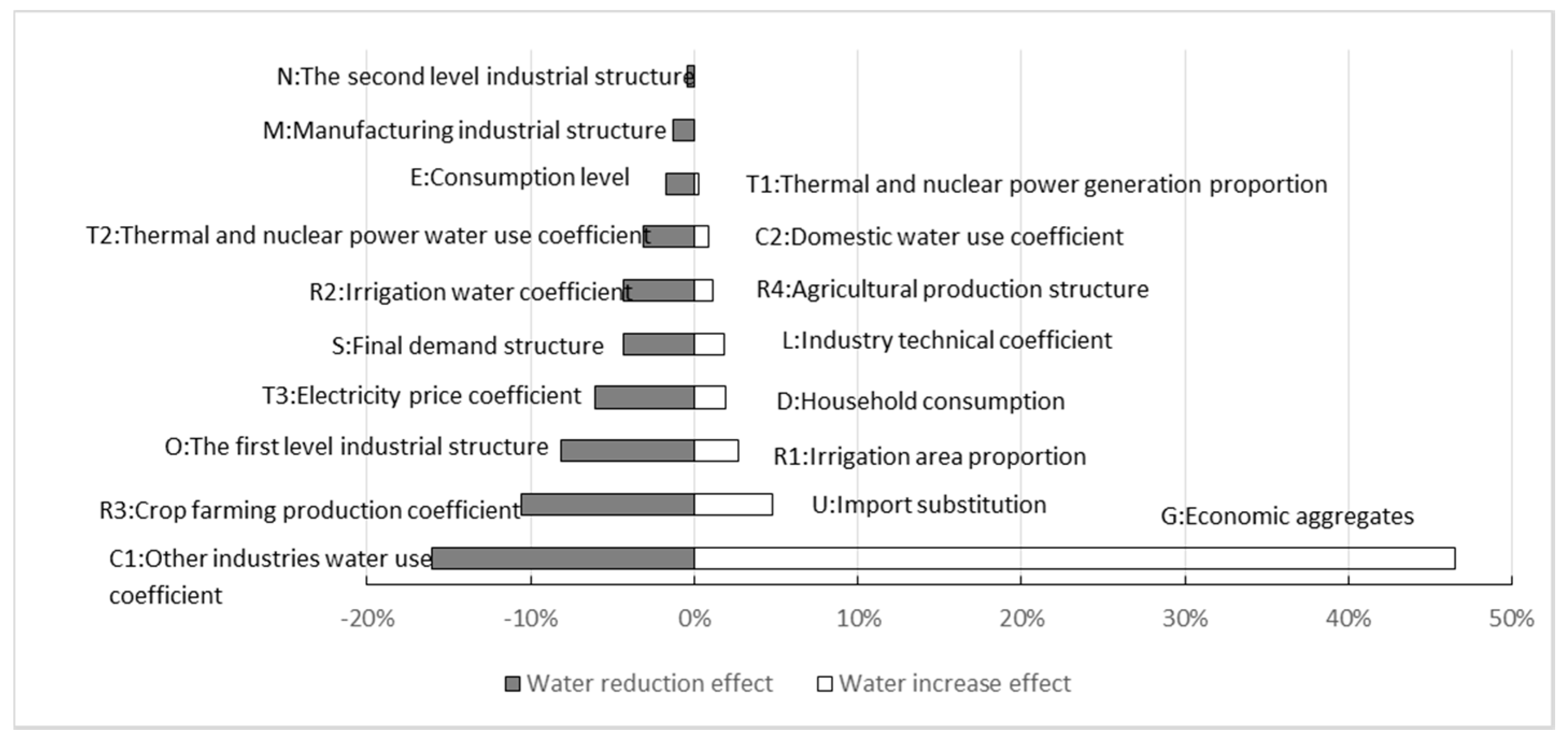
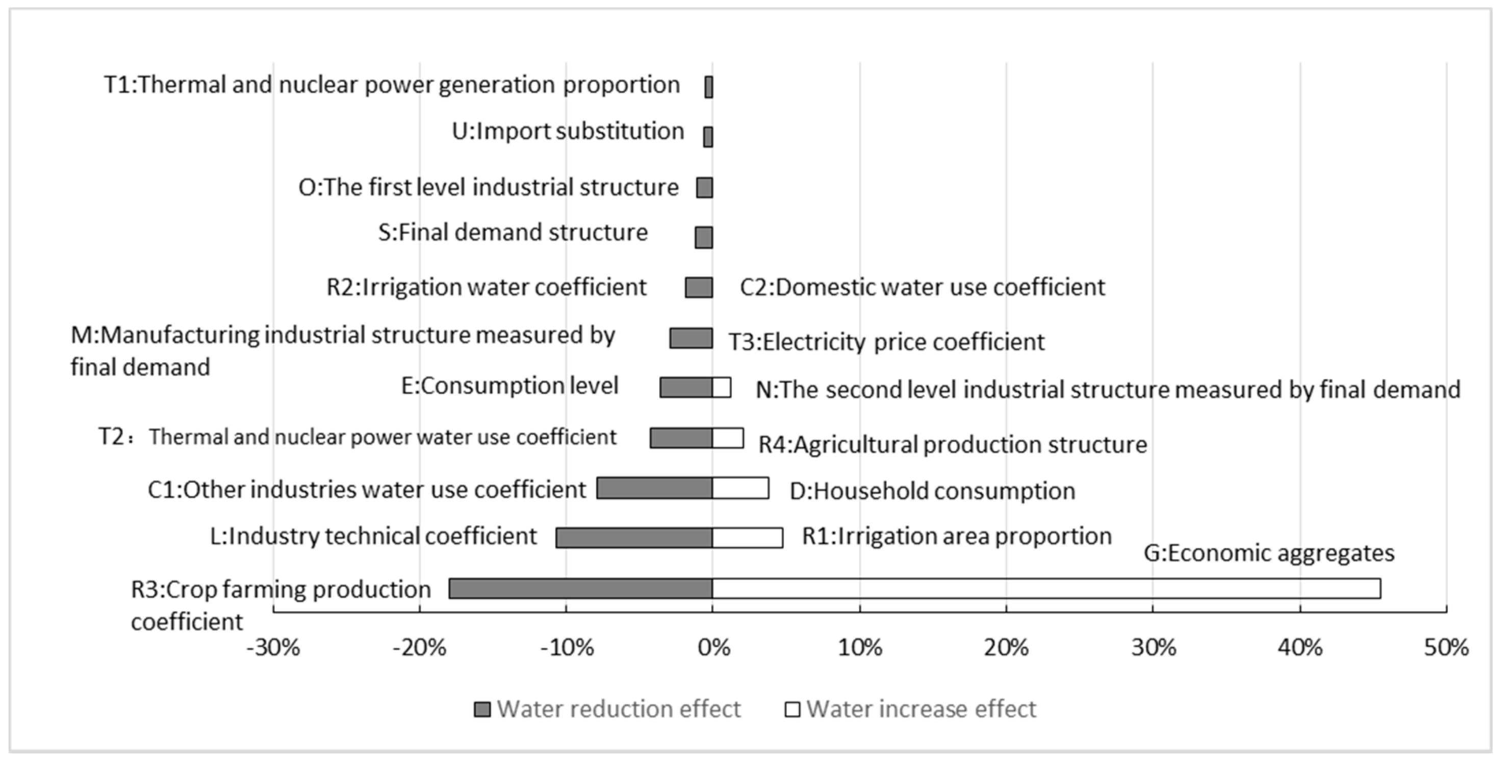
4. Results and Discussions

4.1. Basic Results Analysis

From 2002 to 2007, water use increased by 3.9%. The driving factors are illustrated in Figure 1. Of the 18 factors, 10 had the effect of reducing water use and 8 had the effect of increasing water use. Ten factors that contributed to the reduction total water use are C1 (16%), R3 (10.6%), O (8.1%), T3 (6.1%), S (4.3%), R2 (4.3%), T2 (3.1%), E (1.7%), M (1.3%), N (0.5%). The effects of social and economic factors on water reduction were mainly reflected in the advancement of production technology, advancement of water-saving technology, and adjustment of industrial structure. In other words, more products could be produced per unit of water use. The total effects of the drivers of water reduction decreased water use during this period by 308.4 billion (10⁹) m³, which was 56.1% of the total water use in 2002. Similarly, eight factors increased water use. Evidently, the main factors of the increase in water use were economic and social development, agricultural structure, and increase in irrigation. These factors increased water use by 330 billion (10⁹) m³, which was 60.0% of total water use in 2002.

From 2007 to 2012, water use increased by 5.4%. Figure 2 shows the driving factors and their effect. Of the 18 factors, 11 had the effect of reducing water use and 7 had the effect of increasing water use. Eleven factors that contributed to the reduction in total water use are R3 (18%), L (10.6%), C1 (7.9%), T2 (4.2%), E (3.6%), M (2.9%), R2 (1.8%), S (1.2%), O (1.1%), U (0.6%), T1 (0.5%). The effects of social and economic factors on water reduction were mainly reflected in the advancement in production technology, advancement in water-saving technology, and adjustment in industrial structure. The total water reduction effect reduced water use during this period by 299.4 billion (10⁹) m³, which was 52.4% of total water use in 2007. Similarly, seven factors contributed to the water increasing effect. Evidently, the main factors for the increase in water use were economic and social development, agricultural structure, and increase in irrigation. These factors increased water use by 329.9 billion (10⁹) m³, which was 57.7% of total water use in 2007.

A comparison of these two time periods showed changes in each factor’s effect on water use. The three factors of economic aggregates (G), crop farming production coefficient (R3), and other industries’ water-use coefficient (C1), representing economic scale, agricultural production efficiency, and overall industry water-use efficiency, respectively, had a larger impact on water use. Economic aggregates (G) had always been the largest driving factor for water use, resulting in a water increase effect. Its driving force proportion decreased slightly from 46.6% to 45.5%. The driving force of the intermediate input technical coefficient (L) changed significantly. Between 2002 and 2007, it was a water increase driving factor (increased water use by 1.8%), and between 2007 and 2012, it was a water reduction driving factor (reduced water use by 10.6%). This indicates advancement of production efficiency was directed toward water-saving and gradually became an important driving force.

4.2. The Effect of the Crop Farming Industry

The water-reducing effect of the crop farming industry reduced total water use by 11.1% between 2002 and 2007, and by 13% between 2007 and 2012. The crop farming production coefficient and irrigation water coefficient had a water reduction effect, while the irrigation area proportion and agricultural production structure had a water increasing effect.

Table 3. Technical parameters of agricultural production.

Year	Grain Production (1 Billion Tons)	Irrigation Area Ratio (%)	Irrigation Water Coefficient * (m3/ha)	Crop Farming Production Coefficient ** (Dollar/ha)	Agricultural Production Structure (Crop Farming Proportion, %)
2002	4.571	45.3	26.8	9.1	49.4
2007	5.015	47.4	25.0	10.8	50.4
2012	5.896	51.3	24.2	14.9	52.5

* The irrigation water-use coefficient is determined according to actual irrigated area and amount of irrigation water. The data are from the China Statistical Yearbook [29,30,31], with lower values than those in the Water Resources Bulletin [2,20,21]. ** The crop farming production coefficient here is the reciprocal of the median value calculated in the previous matrix. The average exchange rate was 7.8073 in 2007.

shows the technical parameters of agricultural production. The adjustment of the agricultural production structure (increased proportion of crop farming production) and increase in the proportion of irrigation area led to an increase in grain production and water use. From 2002 to 2007, agricultural grain production increased by 9.7%, and by 17.6% from 2007 to 2012. This was mainly realized by expanding the crop farming area, increasing the irrigation area, and increasing agricultural production efficiency.

The crop farming production coefficient (arable land area occupied per dollar output) reduced water use by 10.6% between 2002 and 2007, and by 18.0% between 2007 and 2012. This indicates an increasingly prominent effect on water use. The irrigation water coefficient reduced water use by 4.3% between 2002 and 2007, and by 1.8% between 2007 and 2012.

With the advance of drought-resistant seed technology and agricultural production technology, as well as continuous improvement in farmland water conservancy facilities, China’s agricultural production efficiency has been consistently improving. The advance in agricultural technology and agricultural water-saving technology offset the aforementioned driving forces for increased water use.

4.3. The Effect of the Power Industry

The water-reducing effect of power production reduced total water use by 9.0% between 2002 and 2007, and by 3.5% between 2007 and 2012; the thermal and nuclear power water-use coefficient reduced water use. Water use of the secondary industries mainly comprises thermal and nuclear power water use, which accounts for more than 30% of industrial water use. Thermal and nuclear power generation was 3.9528 trillion kWh in 2012, which was approximately 2.8 times that in 2002.

Table 4. Technical parameters of the power industry.

Year	Total Power Generation	Thermal and Nuclear Power Generation	Thermal and Nuclear Power Generation Ratio	Electricity Price Coefficient *	Power Industry’s Water-Use Coefficient
	(1 Billion kWh)	(1 Billion kWh)	(%)	(Dollar/kWh)	(m3/kWh)
2002	1654	1363	0.82	0.07	0.027
2007	3278	2785	0.85	0.13	0.018
2012	4938	3990	0.80	0.11	0.011

* The electricity price coefficient here is the reciprocal of the median value calculated in the previous matrix. The average exchange rate was 7.8073 in 2007.

shows the parameters of the power industry. The per unit power output value (power output value/power generation) was 0.07, 0.13, and 0.11 dollar/kWh in 2002, 2007, and 2012, respectively. The power production coefficient led to a reduction in water use of 6.1% and an increase in water use of 1.2% in the two time periods, respectively. This indicates that the increase in per unit power output value could reduce water use, while the decrease in per unit power output value could increase water use. The thermal and nuclear power generation proportion resulted in an increase in water use of 0.2% between 2002 and 2007, and a reduction in water use of 0.5% between 2007 and 2012. This indicates that an increase in the scale of the thermal and nuclear power structure would have a water-increasing effect. In contrast, a reduction in the proportion of thermal and nuclear power could have a water-reducing effect.

Water is a good heat conductor in the power production process. It is used for cooling, which is not a necessary consumable. Although the final demand brought about by economic development increased, and the demand for electricity increased rapidly, the increase in power water use was stable. It did not increase dramatically with increasing power generation because of advances in recycling and water-saving technology and the consistent improvement in the overall water-use efficiency of the power industry.

4.4. The Effect of the Development Mode Transformation

“The transformation of the development mode” mainly refers to the optimization of the economic demand structure, as well as the adjustment of international trade through methods like macro-control. In this study, the transformation of the development mode is decomposed into final demand structure (S), first-level industrial structure (O), second-level industrial structure (N), manufacturing industrial structure (M) measured by final demand, and import substitution (U).

The water-reduction effect brought about by the transformation of the development mode reduced water use by 9.5% from 2002 to 2007 and by 5.3% from 2007 to 2012. Except for import substitution (U) between 2002 and 2007, and the second-level industrial structure (N) between 2007 and 2012, both of which had water-increasing effects, all other factors had water-reduction effects. This indicates that the transformation of economic development was conducive for total water-use control.

The final demand structure (S) during the periods examined is shown in Table 3. In the final demand structure (S), the proportion of fixed capital formation increased continuously. Exports increased from 16.95% to 26.35%, and then dropped to 21.96% in 2012. While government consumption gradually decreased, household consumption also showed a decreasing trend, dropping to 29.05% in 2012. During these periods, China’s economic growth mainly relied on investment and consumption, and the pulling effect of investment and exports gradually increased. The changes in the final demand structure (S) had a significant water-reducing effect, reducing water use by 4.3% between 2002 and 2007, and by 1.2% between 2007 and 2012.

The changes in the first-level industrial structure (O) in final demand were mainly reflected by the decrease in the proportions of the primary and tertiary industries, as well as the increase in the proportion of the secondary industries. Their proportions in 2002, 2007, and 2012 were 9.3:55.8:34.9, 5.1:62.4:32.5, and 4.1:62.1:33.8, respectively (

Table 5. Final demand structure.

Year	Final Demand Structure (S, %)				First-Level Industrial Structure in the Final Demand (O, %)
	Household Consumption	Government Consumption	Fixed Capital	Exports	Primary Industry	Secondary Industry	Tertiary Industry
2002	38.99	17.48	26.58	16.95	9.3	55.8	34.9
2007	29.43	11.02	33.20	26.35	5.1	62.4	32.5
2012	29.05	9.41	39.59	21.96	4.1	62.1	33.8

). This structural change helped reduce water use. Water use declined by 8.1% between 2002 and 2007, and by 1.1% between 2007 and 2012. The first-level industrial structure had a great change and water-reducing effects were significant between 2002 and 2007.

The change in the manufacturing industrial structure (M) in final demand reduced water use by 1.3% between 2002 and 2007, and by 2.9% between 2007 and 2012. The industries that account for a large proportion and show an increasing trend include general-purpose equipment manufacturing, transportation equipment manufacturing, the electric industry, and other electronic equipment manufacturing industries. The industries that also account for a large proportion, but show a decreasing trend include food manufacturing, tobacco processing, textile, clothing, chemical, and other water-intensive industries. Evidently, the manufacturing industrial structure is adjusting to the gradual reduction in the proportion of water-intensive industries and increase in the proportion of low-water industries. Therefore, changes in the manufacturing industrial structure had a water-reducing effect.

The import substitution (U) changes from a water increase driving factor (increased water use by 4.8%) to a water reduction driving factor (reduced water use by 0.6%). The flow of products reflects a “virtual water” flow in international trade. “Virtual water” can reduce total water use by increasing the import of goods with higher virtual water content and reducing the export of products like grains and textiles.

4.5. The Effect of Domestic Living

The influencing factors of domestic water increased water use by 1.1% between 2002 and 2007, and by 0.3% between 2007 and 2012. Among the factors, household consumption (D) was the main factor driving the water-use increase. Increase in household consumption (D) closely relates to population growth. In the two periods, household consumption drove an increase of 1.9% and 3.8% in water use, respectively, and the water-increasing effect showed a rising trend. The level of consumption (E) was the main factor that drove water-use reduction. Thus, as the income level increased, the water-reducing effect of domestic water consumption gradually emerged. Water use driven by level of consumption (E) declined by 1.7% between 2002 and 2007, and by 3.6% between 2007 and 2012. The domestic water use coefficient (C2), that is, per capita domestic water use, had a weak influence on total water use. Water use driven by C2 increased by 0.9% and 0.1%, respectively.

5. Conclusions

The water-comparable non-competitive input–output table for 2002, 2007, and 2012, compiled in this paper can eliminate the influences of pricing factors and imported products on water use and the driving force analysis. An SDA model of the driving factors for water use was conducted, in which 18 factors were considered. The model expressed the driving forces in detail. There were driving factors for both water-increasing and water-reducing effects. Quantifying the driving force of water use is useful for controlling the total water use.

According to this study, economic growth increases water use, but its effect was declining. Advancement of production technology in China between 2002 and 2012 was directed toward water-saving and gradually became an important driving force. The advancement of agricultural technology (increase in agricultural production) and irrigation efficiency offset the increase in water use, thereby realizing an increase in water-use efficiency. The improvement in production technology and water-saving technology played a major role in water-use reduction and increased water-use efficiency in the power industry. This declares that water-saving technologies and production technologies are both crucial for controlling total water use. Transformation of the development mode was an important factor that drove the reduction of water use. The decline in the final consumption structure and the increase in investment had water-reducing effects. Regarding final demand, the decrease in the proportion of primary industries led to obvious water-reducing effects. Controlling the proportion of high water-intensive industries and thermal and nuclear power generation in the economic system was important to save water resources. International trade was also important to alleviate water stress in China.

This research method can be applied to factor decomposition calculation in other fields, and the setting of driving factors can be changed according to the research situation. However, this study relies on the regional input–output tables, which are compiled lagging behind. Thereby the study also has time lag. Furthermore, in many countries and regions there is no industry water-use statistics, which leads to some inaccuracies.

References

1. Du, T.; Kang, S.; Zhang, X.; Zhang, J. China’s food security is threatened by the unsustainable use of water resources in North and Northwest China. Food Energy Secur. 2014, 3, 7–18. [Google Scholar] [CrossRef]
2. The Ministry of Water Resources of China. China Water Resources Bulletin (2002); China Water & Power Press: Beijing, China, 2002. (In Chinese)
3. The Ministry of Water Resources of China. China Water Resources Bulletin (2015); China Water & Power Press: Beijing, China, 2015. (In Chinese)
4. Shang, Y.; Lu, S.; Shang, L.; Li, X.; Wei, Y.; Lei, X.; Wang, C.; Wang, H. Decomposition methods for analyzing changes of industrial water use. J. Hydrol. 2016, 543, 808–817. [Google Scholar] [CrossRef] [Green Version]
5. Xia, Y.; Yang, C.H.; Chen, X.K. Analysis on determining factors of energy intensity in China based on comparable price input-output table. Syst. Eng. Theory Pract. 2009, 29, 21–27. (In Chinese) [Google Scholar] [CrossRef]
6. Guo, C.X. An analysis of the increase of CO2 emission in China—Based on SDA technique. China Ind. Econ. 2010, 12, 47–56. (In Chinese) [Google Scholar] [CrossRef]
7. Sherwood, J.; Clabeaux, R.; Carbajales-Dale, M. An extended environmental input-output lifecycle assessment model to study the urban food-energy-water nexus. Environ. Res. Lett. 2017, 12, 105003. [Google Scholar] [CrossRef]
8. Li, J. A decomposition method of structural decomposition analysis. J. Syst. Sci. Complex. 2005, 18, 210–218. [Google Scholar]
9. Wood, R. Structural decomposition analysis of Australia’s green house gas emissions. Energy Policy 2009, 37, 4943–4948. [Google Scholar] [CrossRef]
10. Carter, H.O.; Ireri, D. Linkage of California-Arizona input-output models to analyze water transfer pattern. In Applications of Input-Output Analysis; Carter, A.P., Brody, A., Eds.; North-Holland Publishing Co.: Amsterdam, The Netherlands, 1972. [Google Scholar]
11. Liu, L.F. Application of Input-output Technology in the adjustment of water price in Beijing. Stat. Decis. 2005, 20, 146–148. (In Chinese) [Google Scholar] [CrossRef]
12. Incera, A.C.; Avelino, A.F.; Solís, A.F. Gray water and environmental externalities: International patterns of water pollution through a structural decomposition analysis. J. Clean. Prod. 2017, 165, 1174–1187. [Google Scholar] [CrossRef]
13. Rose, A.; Chen, C.Y. Sources of change in energy use in the US economy, 1972- 1982: A structural decomposition analysis. Resour. Energy 1991, 13, 1–21. [Google Scholar] [CrossRef]
14. Cazcarro, I.; Duarte, R.; Sanchez-Choliz, J. Economic growth and the evolution of water consumption in Spain: A structural decomposition analysis. Ecol. Econ. 2013, 96, 51–61. [Google Scholar] [CrossRef]
15. Yang, Z.W.; Xu, X.Y.; Chen, W.; Wang, H.R. Dynamic structural decomposition analysis model of water use Evolution II: Application. J. Hydraul. Eng. 2015, 46, 802–810. (In Chinese) [Google Scholar] [CrossRef]
16. Li, W.; Liu, J.H.; Jia, Y.W.; Wang, X.F. Attribution analysis of economic driving factors of social water cycle evolution. J. China Inst. Water Resour. Hydropower Res. 2016, 14, 356–361. (In Chinese) [Google Scholar] [CrossRef]
17. National Bureau of Statistics of China. China Regional Input-Output Table (2002); China Statistical Press: Beijing, China, 2002. (In Chinese)
18. National Bureau of Statistics of China. China Regional Input-Output Table (2007); China Statistical Press: Beijing, China, 2007. (In Chinese)
19. National Bureau of Statistics of China. China Regional Input-Output Table (2012); China Statistical Press: Beijing, China, 2012. (In Chinese)
20. The Ministry of Water Resources of China. China Water Resources Bulletin (2007); China Water & Power Press: Beijing, China, 2007. (In Chinese)
21. The Ministry of Water Resources of China. China Water Resources Bulletin (2012); China Water & Power Press: Beijing, China, 2012. (In Chinese)
22. Skoulikaris, C.; Ganoulis, J. Multipurpose hydropower projects economic assessment under climate change conditions. Fresenious Environ. Bull. 2017, 26, 5599–5607. [Google Scholar]
23. Fan, L.; Liu, G.; Wang, F.; Ritsema, C.J.; Geissen, V. Domestic water consumption under intermittent and continuous modes of water supply. Water Resour. Manag. 2014, 28, 853–865. [Google Scholar] [CrossRef]
24. The Ministry of Water Resources of China & National Bureau of Statistics of China. Bulletin of First National Census for Water; China Water & Power Press: Beijing, China, 2013. (In Chinese)
25. Zhang, Y.G. Economic development pattern change impact on China’s carbon intensity. Econ. Res. J. 2010, 4, 120–133. (In Chinese) [Google Scholar] [CrossRef]
26. Dietzenbacher, E.; Los, B. Structural decomposition analyses with dependent determinants. Econ. Syst. Res. 2000, 12, 497–514. [Google Scholar] [CrossRef]
27. Fujimagari, D. The sources of change in the canadian industry output. Econ. Syst. Res. 1989, 1, 187–202. [Google Scholar] [CrossRef]
28. Betts, J.R. Two Exact, Non-arbitrary and general methods of decomposing temporal change. Econ. Lett. 1989, 30, 151–156. [Google Scholar] [CrossRef]
29. National Bureau of Statistics of China. China Statistical Yearbook (2002); China Statistical Press: Beijing, China, 2002. (In Chinese)
30. National Bureau of Statistics of China. China Statistical Yearbook (2007); China Statistical Press: Beijing, China, 2007. (In Chinese)
31. National Bureau of Statistics of China. China Statistical Yearbook (2012); China Statistical Press: Beijing, China, 2012. (In Chinese)
Figure 1. Driving effects of various factors on water use from 2002 to 2007.
Sustainability 11 02300 g001
Figure 2. Driving effect of various factors on water use from 2007 to 2012.
Sustainability 11 02300 g002