Optimal Design of a Distributed Energy System Using the Functional Interval Model That Allows Reduced Carbon Emissions in Guanzhong, a Rural Area of China

Abstract

Nowadays, rural power supply in China plays an important role in restricting the economic development and improvement of residential living standards. In this study, an interval full-infinite programming rural energy model (IFIP-REM) was developed for supporting distributed energy system (DES) optimal design under uncertainties in rural areas. By affecting the upper and lower bounds of the interval by complex and variable external conditions, IFIP-REM could simulate the influence of external systems. To validate the model, a real case study of DES optimal design in Guanzhong, a rural area of China, was tested and aimed to minimize system cost and constraints of resources, energy supply reliability, and carbon emission mitigation. The data revealed generation of reasonable optimization schemes to obtain interval solutions of IFIP-REM. Compared to centralized energy system (CES), DES reduced electricity purchasing of the municipal grid by 47.5% and extended carbon emission of both upper and lower bounds to [17.13, 44.51] % and [12.42, 36.02] %, respectively. Overall, the proposed model could help managers make decisions of DES optimal design by coordinating conflicts among economic cost, system efficiency, and carbon emission mitigation.

1. Introduction

According to the United Nations Environment Program, energy consumption has increased dramatically in the past few decades, where the architecture sector accounts for about 40% [1,2,3]. The situation is particularly striking in China since the building energy consumption has doubled in just 20 years with average growth rate of 3.70% [4] and an average energy consumption growth rate of 8.56% in rural areas [5,6]. Rural power supply has become an important factor in restricting current rural economic development and improvement of residential living standards. To solve the problem of power supply in rural areas, the government has performed several developments of agricultural networks via upgrading and reconstruction projects. However, many economy and technology-related issues still require solutions, particularly in remote areas and border defense islands. Therefore, it is urgent to seek new solutions while upgrading rural grids [7].

Distributed energy systems (DES) can handle small-scale, short-distance energy supply problems to compensate for the shortcomings of the municipal grid [8]. It is increasingly becoming an attractive option worldwide due to its high efficiency, superior reliability, less investment, and reduced transportation distance [9,10]. Compared to centralized energy systems (CES), DES uses a wider range of technologies containing prime movers, waste heat recovery, energy storage, heat pumps, solar photovoltaic, small wind turbines, and other equipment with renewable energy resources [11,12,13,14,15,16]. DES use renewable energy to reduce dependence on fossil fuel resources and reduce carbon emissions to the atmosphere [17]. Therefore, the development of DES according to local conditions would be an effective measure to promote large-scale utilization of rural renewable energy, maintaining rural natural ecological environment, and improving rural power supply capacity. This, in turn, will be of great significance to the rapid development of the rural economy.

Therefore, numerous studies have been devoted for optimal design of DES. For instance, Liu et al. calculated the optimal operation and explored the economic, energy saving, emission reduction, and peak modulating characteristics of DES under different configurations [18]. Doagou-Mojarrad et al. proposed an optimized method to reduce power loss, energy cost, and pollutant emissions [19]. Falke et al. applied an optimized model on investment planning and operation management of DES to examine the impact of different efficiency measures on total cost and emissions of carbon dioxide equivalent [20]. Liu et al. presented the feasibility of different renewable energy penetrations in DES by establishing the Energy PLAN model in Chongming County, China [21]. Yeşim and Mehmet established a mixed integer linear programming model to improve efficiency and reduce the cost of DES by decreasing energy distribution losses and the transportation cost of energy distribution networks [22]. Wu et al. also considered optimal neighborhoods-scale DES for both supply and demand, as well as optimal combination of building structures within community [23]. However, only a few of them focused on uncertainties in the DES optimal design process. Besides, these studies did not consider carbon emission reductions in the same framework, especially in rural areas. In an actual DES optimal design process, uncertainties exist in various aspects, such as energy-supply activities and economic, technical, equipment cost, system stability, fluctuation of energy demand, and political indicators [24,25,26]. First, renewable energy represented in the literature is affected by uncertainties linked to climate [27]. For example, the output powers of photovoltaic plants suffer from randomness and volatility, which will greatly impact the stable operation of the system. Second, the complexity of DES results from a wide variety of system components, such as equipment associated with power generation, refrigeration, heating, and energy storage. Furthermore, management of energy in DES often requires consideration of economic and reliability constraints in actual situations, and the system must be controlled by constraints of electricity balance to maintain the system’s cold and heat balances. Meanwhile, an energy management for DES should not only consider real-time satisfaction of load requirements, but also premeditate the economics of power supply cost.

Several methods have been developed to study such complexities and uncertainties. For example, interval linear programming (ILP) is employed to deal with problems of interval uncertainties in system analysis [28,29,30,31]. This defines uncertainties in an interval range, determining the upper and lower bounds, and performing system analysis [32,33,34,35]. However, ILP is based on assumptions of the upper or lower determination number (crisp interval) [36]. The crisp interval is then input into the model and the relationship between the final values of the upper and lower bounds with external impact factors cannot be intuitively reflected. In practical problems, the upper and lower of intervals are affected by complex and variable external factors, requiring function intervals to characterize the factors. For example, the purchase cost of equipment would change according to discount rate, defining the ratio of future limited-period expected income in present value. The change in discount rate will then be affected by external uncertainty factors. An effective way for describing these uncertainties would be through function intervals, in which the upper and lower bounds are functions related to several influencing factors. When uncertainty factors are expressed as crisp intervals and function intervals, they lead to the interval full-infinite programming method (IFIP) [37]. IFIP is based on extension of uncertainties as crisp and function intervals with infinite numbers of objective function and constraints. These reflect decision-making objectives directly in the optimization process and solution results, and prevent shortcomings of various methods running separately [38].

Therefore, in this study, an interval full-infinite programming rural energy model (IFIP-REM) was developed to optimize the design of DES in rural areas. IFIP-REM was then applied to a real case in Guanzhong for optimal design of DES, where both energy load and system equipment matching problems were taken into account to identify the optimal energy-using pattern of local energy systems. The IFIP method for dealing with uncertainties was represented as crisp intervals and functional intervals. The determination of outcomes for desired policy associated with rural environment, economic, and energy supply reliability were discussed. The solutions obtained from the case study provide a foundation for decision-making related to the optimal design of DES in rural areas, such as promoting capacity expansion and/or dynamic changes in development planning. The obtained solutions would also be utilized for coordinating economic cost, system efficiency, and solving conflicts among pollutant mitigation and energy supply security interactions under uncertainty.

2. Application

2.1. Problem Description

To promote China’s Western Development Policy and construct the Belt and Road Initiatives, the Ministry of Housing and Urban-Rural Development of the People’s Republic of China issued the act of “Development Plan for the Guanzhong Plain Urban Agglomeration” in 2018. The Guanzhong Plain urban agglomeration is located in the center of inland China (104°57′E~112°56′E, 33°09′N~36°93′N), centered on Xi’an [39]. It is located in a cold temperate zone (National Building Thermal Design Division) with average elevation of about 500 m, and is characterized by four distinct seasons with large temperature differences, long, cold winters, and dry weather [40,41]. The Guanzhong area is the second urban agglomeration in western China with administrative space of around 107.10 × 10³ km², population of 29.80 million, and 1958.42 billion RMB regional GDP as of 2017. It is the most important birthplace of Chinese civilization and the starting point of the ancient Silk Road. Hence, it has a unique strategic position in national modernization and acts as an important fulcrum of the Eurasian Continental Bridge and a gateway to the western region.

Currently, renewable energy usage in Guanzhong is still relatively simple and inefficient. Though solar energy, biomass, and geothermal energy are employed, their efficiency does not exceed 10% [42]. Therefore, it is necessary to reform energy use in rural areas and introduce new energy-saving and environmentally-friendly resources, such as DES, to improve energy problems in rural areas. This would promote the development of rural life and economy. Meanwhile, renewable energy storage space in rural areas will enable better use of distributed energy to move away from fossil energy. Thus, it is necessary to optimize the design of DES in this region according to the actual situation.

The region suffers from several problems. First, the introduction of national strategy of Guanzhong Plain urban agglomeration and the Belt and Road Initiatives have both increased energy consumption in Guanzhong, with a gap in energy supply and demand. Second, the large distance separating the Guanzhong rural area from power stations has led to a relatively fragile distribution network that is vulnerable to emergencies and low power supply reliability. Third, the Guanzhong area suffers from adverse natural conditions and a fragile ecological environment and has high environmental protection requirements. Fourth, it is located deeply inland and is sandwiched between the Qinling Mountains and Loess Plateau. The air dispersion is weak, resulting in increased constraints between the atmospheric environment and air pollution [43].

When designing DES in Guanzhong with a hybrid sustainable energy system, including a multisource, multitechnology, and multiuser environment, many uncertainties and interactions must be systematically evaluated. Many uncertainties exist in various factors and processes associated with power production, conversion, transmission and supply, and energy conversion. If local energy supply does not meet energy demand, some degree of energy supply uncertainties may emerge, and addressing these uncertainties and complexities is important.

2.2. Modeling

The Guanzhong area is rich in renewable energy resources, such as biomass, geothermal sources, and solar. These features can establish the DES study [44]. The target function of the proposed system was to minimize the total system cost. This could be formulated as interval full-infinite programming rural energy model (IFIP-REM) described through Equations (1)–(24):

Objective function:

$$\min f=(C_{Capital}+C_{OM}+C_{Fuel}+C_{Elec}-C_{Sub})$$

(1)

(1) Equipment cost:

$$\begin{array}{ll}{C}_{Capital}& =4/365\times [{\displaystyle {\sum }_i{\displaystyle {\sum }_{u}Maxca{p}_{iu}^{\pm }\times P{N}_i^{\pm }\times CapCos{t}_{iu}^{\pm }\left({\alpha }_i\right)}}\\ & +{\displaystyle {\sum }_{u}MaxCap{C}_u^{\pm }\times PN{C}_u^{\pm }\times CapCost{C}_u^{\pm }\left({\beta }_u\right)}\\ & +{\displaystyle {\sum }_{u}MaxESto{r}_u^{\pm }\times PN{S}_u^{\pm }\times CapCost{S}_u^{\pm }\left({\beta }_u\right)}]\end{array}$$

(2)

(2) Equipment operating cost:

$$\begin{array}{ll}{C}_{OM}& ={\displaystyle {\sum }_s{\displaystyle {\sum }_h{\displaystyle {\sum }_i{\displaystyle {\sum }_{u}O{M}_{iu}^{\pm }\left({\varphi }_{iu}\right)\times G_{shiu}^{\pm }}}}}+{\displaystyle {\sum }_s{\displaystyle {\sum }_h{\displaystyle {\sum }_{u}OM{C}_u^{\pm }\left({\tau }_u\right)\times C{T}_{shu}^{\pm }}}}\\ & +4/365\times {\displaystyle {\sum }_{u}OM{S}_u^{\pm }\left({\tau }_u\right)\times MaxESto{r}_u^{\pm }}\end{array}$$

(3)

(3) Fuel cost:

$$C_{Fuel}={\displaystyle {\sum }_s{\displaystyle {\sum }_h{\displaystyle {\sum }_i{\displaystyle {\sum }_{u}PFue{l}_{iu}^{\pm }\left({\psi }_{iu}\right)\times G_{shiu}^{\pm }/{\eta }_{iu}^{}}}}}$$

(4)

(4) Purchasing electricity cost:

$$C_{Elec}={\displaystyle {\sum }_s{\displaystyle {\sum }_{h}PEle{c}_h^{}\times E{P}_{sh}^{\pm }}}$$

(5)

(5) Subsidy:

$$\begin{array}{c}{C}_{Sub}=4/365\times {\displaystyle {\sum }_i{\displaystyle {\sum }_{u}PSu{b}_{iu}^{\pm }\times MaxCa{p}_{iu}^{\pm }/Tlif{e}_i^{\pm }}}\\ +{\displaystyle {\sum }_s{\displaystyle {\sum }_h{\displaystyle {\sum }_i{\displaystyle {\sum }_{u}PSub{V}_{iu}^{\pm }\left({\sigma }_{iu}\right)\times G_{shiu}^{\pm }}}}}\end{array}$$

(6)

(6) Carbon emissions:

a. Carbon emissions of this system:

$$Ptl={\displaystyle {\sum }_s{\displaystyle {\sum }_{h}E{P}_{sh}^{\pm }\times cefg}}+{\displaystyle {\sum }_s{\displaystyle {\sum }_h{\displaystyle {\sum }_i{\displaystyle {\sum }_u{G}_{shiu}^{\pm }\times ce{f}_{iu}/{\eta }_{iu}}}}}$$

(7)

b. Carbon emissions from centralized energy system:

$$\begin{array}{ll}Ctptl=& {\displaystyle {\sum }_s{\displaystyle {\sum }_{h}E{D}_{sh,u=cold}^{\pm }\times cefcg}}/md+\\ & {\displaystyle {\sum }_s{\displaystyle {\sum }_{h}E{D}_{sh,u=heat}^{\pm }\times cefng}}/mr+{\displaystyle {\sum }_s{\displaystyle {\sum }_{h}E{D}_{sh,u=elec}^{\pm }\times cefg}}\end{array}$$

(8)

Subject to:

(1) Maximum power constraints for equipment:

$${\displaystyle {\sum }_s{\displaystyle {\sum }_h{\displaystyle {\sum }_i{\displaystyle {\sum }_u{G}_{shiu}^{\pm }}}}}\le {\displaystyle {\sum }_i{\displaystyle {\sum }_{u}P{N}_i^{\pm }\times MaxCa{p}_{iu}^{}}}$$

(9)

$${\displaystyle {\sum }_s{\displaystyle {\sum }_h{\displaystyle {\sum }_{u}C{T}_{shu}^{\pm }}}}\le {\displaystyle {\sum }_{u}PN{C}_u^{\pm }\times MaxCap{C}_u^{}}$$

(10)

$$\lambda \times {\displaystyle {\sum }_s{\displaystyle {\sum }_h{\displaystyle {\sum }_i{\displaystyle {\sum }_u{G}_{shi=NG,u=heat}^{\pm }}}}}\le {\displaystyle {\sum }_s{\displaystyle {\sum }_h{\displaystyle {\sum }_i{\displaystyle {\sum }_u{G}_{shi=NG,u=elec}^{\pm }}}}}$$

(11)

(2) Solar photovoltaic panel generation constraints:

$${\displaystyle {\sum }_s{\displaystyle {\sum }_h{\displaystyle {\sum }_i{\displaystyle {\sum }_u{G}_{s,h,i=PV,u=elec}^{\pm }}}}}\le {\displaystyle {\sum }_s{\displaystyle {\sum }_h{\displaystyle {\sum }_i{\displaystyle {\sum }_{u}P{N}_{i=PV}^{\pm }\times SA\times S{I}_{sh}^{\pm }\times {\eta }_{i=PV,u}^{}}}}}$$

(12)

(3) Energy conversion equipment conversion constraints:

$${\displaystyle {\sum }_s{\displaystyle {\sum }_h{\displaystyle {\sum }_i{\displaystyle {\sum }_u{\omega }_{u=cold}^{}{\displaystyle {\sum }_i{G}_{s=sum,h,i,u=heat}^{\pm }}}}}}={\displaystyle {\sum }_s{\displaystyle {\sum }_h{\displaystyle {\sum }_{u}C{T}_{s=sum,h,u=heat}^{\pm }}}}$$

(13)

$${\displaystyle {\sum }_s{\displaystyle {\sum }_h{\displaystyle {\sum }_i{\displaystyle {\sum }_u{\omega }_{u=elec}^{}{\displaystyle {\sum }_i{G}_{s=sum,h,i,u=elec}^{\pm }}}}}}={\displaystyle {\sum }_s{\displaystyle {\sum }_h{\displaystyle {\sum }_{u}C{T}_{s=sum,h,u=elec}^{\pm }}}}$$

(14)

$${\displaystyle {\sum }_s{\displaystyle {\sum }_h{\displaystyle {\sum }_i{\displaystyle {\sum }_u{\omega }_u^{}{\displaystyle {\sum }_i{G}_{s=spr/aut/win,h,i,u}^{\pm }}}}}}={\displaystyle {\sum }_s{\displaystyle {\sum }_h{\displaystyle {\sum }_{u}C{T}_{s=spr/aut/win,h,u}^{\pm }}}}$$

(15)

(4) Storage equipment constraints:

Energy storage equipment at h = 1:

$${\displaystyle {\sum }_s{\displaystyle {\sum }_h{\displaystyle {\sum }_{u}ESto{r}_{s,h=1,u}^{\pm }}}}=0$$

(16)

$${\displaystyle {\sum }_s{\displaystyle {\sum }_h{\displaystyle {\sum }_{u}ISto{r}_{s,h=1,u}^{\pm }}}}\ge 0$$

(17)

$${\displaystyle {\sum }_s{\displaystyle {\sum }_h{\displaystyle {\sum }_{u}OSto{r}_{s,h=1,u}^{\pm }=0}}}$$

(18)

Energy storage equipment at h>1:

$${\displaystyle {\sum }_s{\displaystyle {\sum }_h{\displaystyle {\sum }_{u}ESto{r}_{shu}^{\pm }}}}={\displaystyle {\sum }_s{\displaystyle {\sum }_h{\displaystyle {\sum }_{u}ESto{r}_{s,h-1,u}^{\pm }+{\upsilon }_u^{}\times ISto{r}_{s,h-1,u}^{\pm }-OSto{r}_{s,h-1,u}^{\pm }}}}$$

(19)

$$0\le {\displaystyle {\sum }_s{\displaystyle {\sum }_h{\displaystyle {\sum }_{u}ESto{r}_{shu}^{\pm }+{\upsilon }_u^{}\times ISto{r}_{s,h-1,u}^{\pm }-OSto{r}_{s,h-1,u}^{\pm }}}}\le {\displaystyle {\sum }_{u}MaxESto{r}_u^{\pm }}$$

(20)

$$0\le {\displaystyle {\sum }_s{\displaystyle {\sum }_h{\displaystyle {\sum }_{u}ESto{r}_{shu}^{\pm }}}}\le {\displaystyle {\sum }_{u}MaxESto{r}_u^{\pm }}$$

(21)

(5) Energy balance constraints:

$${\displaystyle {\sum }_s{\displaystyle {\sum }_h{\displaystyle {\sum }_{u}C{T}_{sh,u=elec}^{\pm }+E{P}_{sh}^{\pm }+OSto{r}_{sh,u=elec}^{\pm }}}}\ge {\displaystyle {\sum }_s{\displaystyle {\sum }_h{\displaystyle {\sum }_{u}ISto{r}_{sh,u=elec}^{\pm }+E{D}_{sh,u=elec}^{\pm }+C{T}_{sh,u=cold}^{\pm }\times {\gamma }^{}}}}$$

(22)

$$\begin{array}{l}{\displaystyle {\sum }_s{\displaystyle {\sum }_h{\displaystyle {\sum }_{u}C{T}_{sh,u=heat/cold}^{\pm }+{\displaystyle {\sum }_s{\displaystyle {\sum }_h{\displaystyle {\sum }_{u}OSto{r}_{sh,u=heat/cold}^{\pm }}}}}}}\ge \\ {\displaystyle {\sum }_s{\displaystyle {\sum }_h{\displaystyle {\sum }_{u}ISto{r}_{sh,u=heat/cold}^{\pm }+{\displaystyle {\sum }_s{\displaystyle {\sum }_h{\displaystyle {\sum }_{u}E{D}_{sh,u=heat}^{\pm }}}}}}}\end{array}$$

(23)

(6) Carbon emission reduction constraint:

$$\begin{array}{l}{\displaystyle {\sum }_s{\displaystyle {\sum }_h{\displaystyle {\sum }_{u}E{P}_{sh}^{\pm }}}}\times cefg+{\displaystyle {\sum }_s{\displaystyle {\sum }_h{\displaystyle {\sum }_i{\displaystyle {\sum }_u{G}_{shiu}\times ce{f}_{iu}/{\eta }_{iu}}}}}\le \\ {\displaystyle {\sum }_s{\displaystyle {\sum }_h{\displaystyle {\sum }_{i}E{D}_{sh,i=cold}}}}\times cefcg\times \left(1-rt\right)/md+\\ {\displaystyle {\sum }_s{\displaystyle {\sum }_h{\displaystyle {\sum }_{i}E{D}_{sh,i=heat}}}}\times cefng\times \left(1-rt\right)/mr+{\displaystyle {\sum }_s{\displaystyle {\sum }_h{\displaystyle {\sum }_{i}E{D}_{sh,i=elec}}}}\times cefg\times \left(1-rt\right)\end{array}$$

(24)

The meanings of symbols and letters are shown in Appendix A, and the methodology is shown in Appendix B.

The construction area was set to 50.66 × 10³ m² in Guanzhong rural area. The cold and heat loads were simulated by EnergyPlus 8.6 software, and the electrical load was obtained through a questionnaire survey in search region (

Table 1. Hourly operation table of household electrical appliances in spring or autumn.

Equipment	Power /W	Hour: From 1 to 24
		1	2	3	4	5	6	7	8	9	10	11	12	13	14	15	16	17	18	19	20	21	22	23	24
Refrigerator	120	1	1	1	1	1	1	1	1	1	1	1	1	1	1	1	1	1	1	1	1	1	1	1	1
Television	200										1	1	1	1			1	1	1	1	1	1	1	1
Humidifier	30
Electro bike	100	1	1	1	1	1	1	1														1	1	1	1
Light	100							3												2	1	1	3	3	1
Computer	300																				1	1	1	1	1
Electric kettle	1200								1											1	1
Induction cooker	2000								1				1							1
Electric cooker	800												1							1
Kitchen ventilator	300												1							1
Microwave oven	1200												1							1
Electric heater	2000
Bathroom master	1200																					1
Washing machine	170											1
Total/W		220	220	220	220	220	220	520	3320	120	320	490	4620	320	120	120	320	320	320	6020	1920	2020	1020	1050	620

,

Table 2. Hourly operation table of household electrical appliances in summer.

Equipment	Power /W	Hour: From 1 to 24
		1	2	3	4	5	6	7	8	9	10	11	12	13	14	15	16	17	18	19	20	21	22	23	24
Refrigerator	120	1	1	1	1	1	1	1	1	1	1	1	1	1	1	1	1	1	1	1	1	1	1	1	1
Television	200												1	1			1	1	1	1	1	1	1	1
Humidifier	30
Electro bike	100	1	1	1	1	1	1	1														1	1	1	1
Light	100						3														2	2	1	1	1
Computer	300																				1	1	1	1	1
Electric kettle	1200							1												1	1
Induction cooker	2000							1						1						1
Electric cooker	800													1						1
Kitchen ventilator	300													1						1
Microwave oven	1200													1						1
air conditioning	1200												1	1	1					1	1	1	1	1
Bathroom master	1200
Washing machine	170
Total/W		220	220	220	220	220	550	3520	120	120	120	120	1520	5820	1320	120	320	320	320	7020	3320	2220	2020	2020	620

and

Table 3. Hourly operation table of household electrical appliances in winter.

Equipment	Power /W	Hour: From 1 to 24
		1	2	3	4	5	6	7	8	9	10	11	12	13	14	15	16	17	18	19	20	21	22	23	24
Refrigerator	120	1	1	1	1	1	1	1	1	1	1	1	1	1	1	1	1	1	1	1	1	1	1	1	1
Television	200										1	1	1	1			1	1	1	1	1	1	1	1
Humidifier	30	1	1	1	1	1	1	1														1	1	1	1
Electro bike	100	1	1	1	1	1	1	1														1	1	1	1
Light	100								3										2	2	1	1	3	3	1
Computer	300																				1	1	1	1	1
Electric kettle	1200								1											1	1
Induction cooker	2000								1					1						1
Electric cooker	800													1						1
Kitchen ventilator	300													1						1
Microwave oven	1200													1						1
Electric heater	2000																					1
Bathroom master	1200																					1
Washing machine	170											1
Total/W		250	250	250	250	250	250	250	3620	120	320	490	320	4620	120	120	320	320	520	6020	1920	4050	1050	1050	650

Notes: Numbers in this table are the number of operating pieces equipment at each time.

). There is little difference in electrical load in spring and autumn, as shown in Table 1. EnergyPlus is a full-featured building energy analysis software that can be used to simulate the building’s running energy consumption. In this study, the following data was entered into the software: (1) Building-related data, including geographic location, time zone, and structure; (2) Equipment data within the building; (3) Meteorological data for the study area. Finally, the energy requirements of the research objective can be obtained through software calculation. The solar energy resources data were extracted from the “Standard Meteorological Data Book of Buildings” [45]. The biomass boiler and ground source heat pump could only be employed in winter and summer seasons [46]. DES equipment is complex, so the equipment is divided into the following categories: (a) energy production equipment: internal combustion generating set (NG), solar photovoltaic panel (PV), biomass boiler (BB); (b) energy conversion equipment: ground source heat pump (GP), absorption chiller (AC), heat exchanger (HE); (c) energy conversion equipment: cold storage equipment (CS), heat storage tank (HS), and battery (BA). This categorization was performed according to government reports, statistical yearbooks, previous research results, equipment product research, and other means to summarize the technical parameters and financial characteristics of various equipment (

Table 4. Summary of equipment parameters.

Equipment	Efficiency			Equipment Cost/RMB/KWh	Operating Cost/RMB/KWh	Lifetime/Year
	L	R	D
NG	--	0.50	0.35	[6625.60(1+α), 9234.40(1+α)]	[0.06(1+ϕ), 0.08(1+ϕ)]	30
PV	--	--	0.16	[6475.20(1+α), 9024.80(1+α)]	[8.40 × 10-3(1+ϕ), 1.2 × 10-3(1+ϕ)]	30
BB	--	0.85	--	[1158.90(1+α), 1615.10(1+α)]	[0.07(1+ϕ), 0.09(1+ϕ)]	20
GP	5.00	4.40	--	[8340.10(1+β), 11623.90(1+β)]	[8.70 × 10-3(1+τ), 11.3 × 10-3(1+τ)]	20
AC	1.20	--	--	[1230.70(1+β), 1715.30(1+β)]	[0.007(1+τ), 0.009(1+τ)]	20
HE	--	0.98	--	[167.90(1+β), 234.10(1+β)]	[1.80 × 10-3(1+τ), 2.60 × 10-3(1+τ)]	20
CS	0.65	--	--	[158.70(1+β), 221.30(1+β)]	[0.17(1+τ), 0.23(1+τ)]	20
HS	--	0.82	--	[75.20(1+β), 104.80(1+β)]	[0.15(1+τ), 0.21(1+τ)]	20
BA	--	--	0.85	[1488.90(1+β), 2075.10(1+β)]	[6.93(1+τ), 9.67(1+τ)]	13.5

Notes: L, R, and D represent cold, heat, and electricity, respectively. α is energy production equipment depreciation rate. β is energy conversion/storage equipment depreciation rate. φ is energy production equipment discount rate. τ is energy conversion/storage equipment discount rate.

).

In this DES, NG and PV generate electricity to supply power to users, and heat generated by NG is recovered by the waste heat storage equipment to directly supply heat load or to supply cold load. When the amount of electricity generated by this system cannot meet the demand of electric load, it is supplemented by the power grid, and when electricity generation is greater than electricity load, it is stored in a battery. In the supply of cold or heat load in this system, when the supply of cold and heat energy of system is greater than the demand of cold or heat load, the excess cold or heat is stored in energy storage equipment; if the cold or heat load requirements are not met, the energy storage equipment is used according to operating criteria, or supplemented by electrical energy conversion. The energy flow chart of the DES designed in this paper is shown in Figure 1. In addition, we compare and analyze the carbon emissions of the CES and DES constructed in this study combined with renewable energy. The compositions of these two systems are shown in

Table 5. Description of the energy systems.

Energy System	System Composition
CES	Power grid + Internal combustion generating set + Absorption chiller + Waste heat boiler + Energy storage system
DES	Power grid + Internal combustion generating set + Absorption chiller + Heat exchanger + Renewable energy equipment + Energy storage system

.

The optimal design process first determines the availability of local resources and selection of corresponding equipment to establish the optimal design model with total cost of the system as the goal. Then, LINGO13.0 (Linear Interactive and General Optimizer 13.0) is used to program and solve the model. The optimal solution of the model is obtained by inputting relevant parameters. LINGO is a comprehensive tool that makes building and solving linear, nonlinear, and integer-optimized models faster, easier, and more efficient, which provides a fast solver engine to illustrate and solve optimization models [47]. In general, using LINGO to solve an operational research problem can be divided into the following two steps: (1) According to the actual problem, establish a mathematical model, use mathematical modeling method to establish an optimization model; (2) LINGO is used to solve the optimization model. Mainly based on LINGO, we translate the mathematical model into a computer language, and solve it with a computer [48]. Figure 2 shows the optimal configuration of IFIP-REM flow. The optimization process would first determine the available resources and corresponding equipment to establish the optimal configuration model with minimum total system cost as the objective function. The model provides the optimal solution and configuration model of the DES.

3. Results and Discussion

The interval full-infinite programming rural energy model (IFIP-REM) was developed to first optimize design the DES and was then applied to Guanzhong. The relationship between the cost of cold, heat, electricity, and system equipment configuration required by users of IFIP-REM solution was established. The interactions among system equipment configuration, cost, and system energy consumption were considered. In this paper, a typical daily load for each season was selected. Because there are 8760 hours in a year, if the energy supply and demand balance of each hour is used as a constraint in optimal design model, after inputting other nonlinear constraints and objective functions, the model will become a complex nonlinear optimization problem. Solving such a model with a general computer will result in difficulty, i.e., the solution efficiency is low, and the solution quality is unstable. Therefore, in the modeling process, it is necessary to appropriately compress the input quantity of energy supply and demand. The compression time dimension is closely related to the energy load characteristics of the system’s terminal. Because the terminal energy load of the study area has a large quarterly difference, the time scale is compressed into four representative seasons, thus reducing the calculation points to 96.

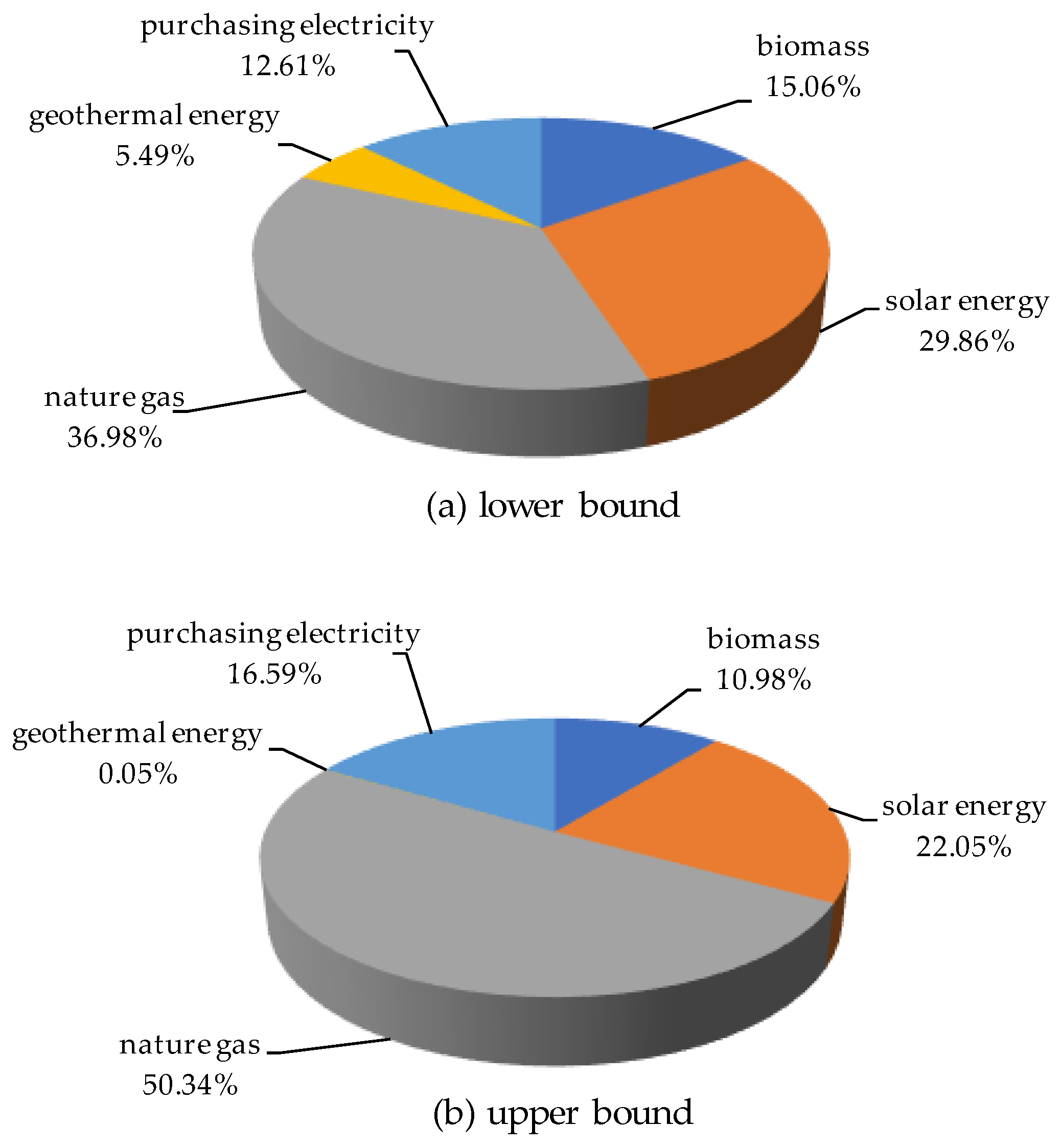
3.1. Energy Consumption

The energy supply scheme’s lower and upper bounds are presented in Figure 3. The energy resources used in Guanzhong can be divided into five types. Natural gas and solar energy ranked first and second with proportions of 36.98% and 50.34%, respectively. In the lower bound supply, geothermal energy accounts for 5.49%. In contrast, geothermal energy of the upper bound supply only accounts for 0.05% of the total energy. This is due to the optimal design meeting the minimum total cost of the system. In addition, because the DES uses natural gas as an energy source in internal combustion engines, natural gas consumption showed the greatest values. These data suggested that imported renewable energy played a significant role in IFIP-RES, particularly when energy demand reached the lower bound.

3.2. Optimized Model

The optimal configuration pattern of the proposed system in terms of cold, heat, and electricity was obtained by calculating IFIP-REM. With four distinct seasons in the Guanzhong area, no requirement for heat or cold in spring and autumn were required, but it is necessary to provide heat and cold in summer and winter to improve residents’ living conditions. The three possible patterns were discussed below.

Figure 4 depicts cold balance patterns for the DES on a typical summer day. During operation of the system, the cold load was mainly met by internal combustion engines, solar photovoltaic panels, and grid power conversion to absorption chillers. User’s cold demand peaked between 13:00 and 20:00 with no fluctuations at other times. As user’s energy demand decreases, the number of ground source heat pump units configured by the system was small. This occurred due to automatic system optimization. Through ground source heat pump and absorption chiller processes, electricity was converted into cold load and then supplied to users. In some periods, excess cold load was generated and stored by ice-storage devices. Since the energy storage efficiency was 0.65, the cold energy released by ice storage devices was lower than the stored cold energy, and no energy was wasted during the cold conversion process. Figure 5 represents the heat balance pattern for the DES on a typical winter day. The heat generated by biomass boilers and internal combustion engines was supplied to users after conversion by heat exchangers. Since the conversion efficiency was 0.98, no energy was wasted during the heating process.

Figure 6 illustrates the electricity balance for a typical day of DES operation in the four seasons. The electricity consumption increased as residents used more appliances during the morning, day, and night. Before these periods, the system stored electricity in advance to reduce the exertion of power generation equipment. The storage efficiency of the battery was 0.85. Hence, the amount of electricity flowing into the batteries was also higher than that flowing out of batteries. Solar radiation intensity reached photovoltaic panel power generation requirements and could operate at full capacity. The electricity generated by photovoltaic panels was directly regulated and controlled by the controller and sent directly to DC and AC loads. When solar photovoltaic panels were excessively utilized at certain periods, electricity other than load power will temporarily be stored in the battery. When the system is short of electricity, the battery can be invoked as a power source to supply the load. Considering the limited capacity of the battery, the system was connected to the municipal grid to ensure normal load. On the other hand, the system stores electric energy during low-voltage periods and sells electricity to the grid during peak hours while ensuring self-use. This might increase the economics of the system while cutting peaks and filling valleys. As we can see in Figure 6, during spring and autumn, because of the lack of cold and heat load demand, only solar photovoltaic panels, storage batteries, and municipal power grids provide electricity for users in this system. The supply and demand are relatively balanced, and basically no power loss occurs. In summer without heat load, absorption chillers can use internal combustion. The refrigeration efficiency of absorption chillers is high, and the coefficient of performance value can reach 1.30, which ensures high system energy utilization efficiency. In the winter, we can see that there is an excess of electric energy. This is because the system needs to generate heat by using internal combustion generators to meet users’ heat demands. Therefore, the power consumption of the system is increased by taking extra power from the grid.

3.3. Carbon Emission

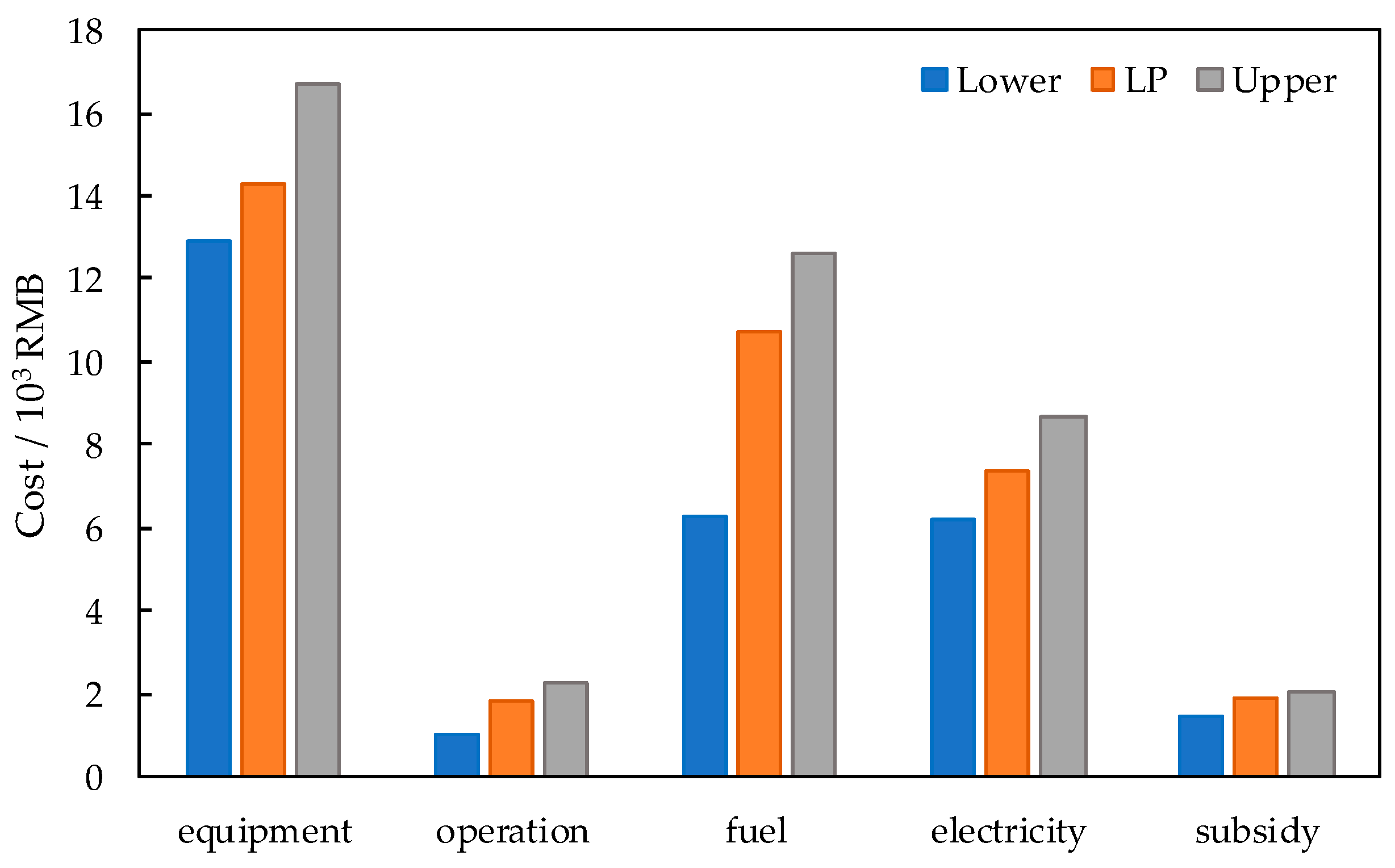
Figure 7 depicts carbon emissions of the DES and CES during the four seasons. The DES showed better reduction in carbon emission than CES, and the carbon reduction rate is [22.73, 31.05] %. In the CES, carbon emissions in spring and autumn were less (4.90 × 10³ and 6.83 × 10³ kg, respectively). The largest values were obtained during winter ([9.45, 13.10] × 10³ kg). In spring and autumn, users utilized no heating or cooling. Carbon discharge increased due to users’ cold and heat loads in summer and winter. However, the carbon emission curve of the DES appeared relatively stable with discharge amounts fluctuating between 3.81× 10³ kg and 5.98 × 10³ kg in spring, summer, and autumn. Carbon discharge amounts rose sharply and discharge was recorded as [6.27, 10.06] × 10³ kg in winter. Because heat generated by biomass boilers and internal combustion engines supplied users after conversion by heat exchangers, carbon discharge rose rapidly.

The purchased electricity from the municipal grid by the DES and CES reached [12.49, 17.38] × 10³ kWh and [23.80, 33.16] × 10³ kWh, respectively. Hence, the DES purchased less electricity from the municipal grid to ensure the reliability of energy usage. The CES consumed more electricity because it required electricity for providing users with heat and cold loads, and thus consumed more power than the DES. Based on the latest coal consumption rates of 6 × 10³ kW and above (326 g/kWh) published by the National Energy Administration, the DES reduced the burning of standard coal by [3687.06, 5144.28] kg per year through clean energy use. Relevant data suggested that natural gas power generation had obvious advantages over coal-fired power in terms of reducing carbon emissions.

3.4. System Cost

The purpose of this study is to minimize the system cost based on optimized results. By optimizing the configuration of the proposed system, total system costs in terms of equipment, operation, fuel, procurement, and subsidies should be minimized. Figure 8 presents the composition of the system cost’s lower and upper bounds under optimal design circumstances. The total cost of this system hovered between RMB 24.82 × 10³ and 39.85 × 10³. Equipment, fuel, and electricity purchase costs accounted for the majority (RMB [12.92, 16.70] × 10³, [6.30, 12.65] × 10³ and [6.22, 8.66] × 10³, respectively). In addition, the cost of renewable energy equipment accounted for [19.82, 63.95] % of total equipment cost. The high price of renewable energy equipment coupled with the lack of subsidies related to DES policies led to the inability of the system to prioritize renewable energy equipment during optimization. The use of renewable energy DES in rural areas would not only solve the daily power needs of thousands of people, but also maximize environmental protection.

3.5. Comparison of DES Model Results Using Linear Programming (LP) and IFIP Method

Figure 9 shows the composition of system cost under optimal design conditions after optimizing DES in Guanzhong rural area of China using the LP and IFIP methods. As seen from Figure 9, equipment cost and fuel cost fluctuate in the optimization process. Combined with the above result-based analysis, it can be indirectly concluded that under the constraints of carbon emissions, in order to meet the demand for energy, the system uses renewable energy equipment for energy supply, which leads to a sharp increase in the equipment cost of this system. The carbon emission reduction effect of the distributed energy system is obvious. Compared with CES, the carbon emission reduction rate optimized by the LP method is 28.50%, while that by IFIP method is [22.71, 31.05] %. Results calculated by the LP method are just within the range of the results calculated by the IFIP method, indicating that the IFIP method can reflect the problems in the process of system optimization more comprehensively and completely than the LP method. IFIP addresses multiple uncertainties in costs, impact factors, and system objectives (decisions, crisp interval and function interval). This model inherits the advantages of LP and full-infinite programming and can directly reflect the objective function and uncertainty in the optimization process and solution.

4. Conclusions

An interval full-infinite programming rural energy model (IFIP-REM) was developed and applied to the distributed energy system (DES) in a rural area. IFIP-REM was applied to Guanzhong to minimize the system cost, meet the high energy demand, achieve better system equipment capacity, moderate equipment cost, and elevate efficiency. The optimal allocation model of the DES considered the abundant renewable energy in rural areas.

Comparison between the traditional centralized energy system and distributed energy system indicated that the allocation pattern of the DES in Guanzhong could be defined according to IFIP-REM calculations. On the other hand, the DES could reduce electricity purchasing from the municipal grid by 47.5% when compared to the CES. The upper and lower bounds of reduction in carbon emissions of the DES reached [17.13, 44.51] % and [12.42, 36.02] %, respectively. The DES was found to be suitable for rural areas rich in renewable energies. The government should introduce relevant laws and policies to support the construction of new energy conversion sources and invest in new projects. In the long run, this should enhance economic and environmental benefits. These findings would help decision makers in discussing alternative energy supplies, renewable energy matching, system cost, and carbon emission mitigation.

For the first time, we attempted to apply the IFIP method to the optimal design of a rural DES considering the increasingly complex and volatile situation in Guanzhong. However, this method still has space for improvement. A major limitation of this model consisted of only using functional intervals linearly related to its factors. Nonlinearities in the DES optimization process exist, so it is necessary to investigate these systems in more depth. Coping with IFIP problems and multiple independent variables will be the focus of future research.

References

1. Besir, A.B.; Cuce, E. Green roofs and facades: A comprehensive review. Renew. Sustain. Energy Rev. 2018, 82, 915–939. [Google Scholar] [CrossRef]
2. Sun, L.; Hu, J.; Jin, H. Research and Application of Distributed Energy Integration Optimization for Sino-German Building in the Cold Area of China. IFAC-PapersOnLine 2018, 51, 90–95. [Google Scholar] [CrossRef]
3. Liu, Z.; Xu, W.; Zhai, X.; Qian, C.; Chen, X. Feasibility and performance study of the hybrid ground-source heat pump system for one office building in Chinese heating dominated areas. Renew. Energy 2017, 101, 1131–1140. [Google Scholar] [CrossRef]
4. Wei, Y.; Zhang, X.; Shi, Y.; Xia, L.; Pan, S.; Wu, J.; Han, M.; Zhao, X. A review of data-driven approaches for prediction and classification of building energy consumption. Renew. Sustain. Energy Rev. 2018, 82, 1027–1047. [Google Scholar] [CrossRef]
5. Wang, R.; Jiang, Z. Energy consumption in China’s rural areas: A study based on the village energy survey. J. Clean. Prod. 2017, 143, 452–461. [Google Scholar] [CrossRef]
6. Chen, C.; Li, Y.; Huang, G. Interval-fuzzy municipal-scale energy model for identification of optimal strategies for energy management A case study of Tianjin, China. Renew. Energy 2016, 86, 1161–1177. [Google Scholar] [CrossRef]
7. Jian, Y.; Xu, Y.; Wu, H.; Yin, D. Economic power supply radius under different distribution transformer installation in rural low-voltage network. Trans. Chin. Soc. Agric. Eng. 2013, 29, 190–195. [Google Scholar]
8. Rieder, A.; Christidis, A.; Tsatsaronis, G. Multi criteria dynamic design optimization of a small scale distributed energy system. Energy 2014, 74, 230–239. [Google Scholar] [CrossRef]
9. Zhou, Z.; Zhang, J.; Liu, P.; Li, Z.; Georgiadis, M.C.; Pistikopoulos, E.N. A two-stage stochastic programming model for the optimal design of distributed energy systems. Appl. Energy 2013, 103, 135–144. [Google Scholar] [CrossRef]
10. Akorede, M.F.; Hizam, H.; Pouresmaeil, E. Distributed energy resources and benefits to the environment. Renew. Sustain. Energy Rev. 2010, 14, 724–734. [Google Scholar] [CrossRef] [Green Version]
11. Han, J.; Ouyang, L.; Xu, Y.; Zeng, R.; Kang, S.; Zhang, G. Current status of distributed energy system in China. Renew. Sustain. Energy Rev. 2016, 55, 288–297. [Google Scholar] [CrossRef]
12. Fujimoto, Y.; Kikusato, H.; Yoshizawa, S.; Kawano, S.; Yoshida, A.; Wakao, S.J.; Murata, N.; Amano, Y.; Tanabe, S.; Hayashi, Y. Distributed energy management for comprehensive utilization of residential photovoltaic outputs. IEEE Trans. Smart Grid 2018, 9, 1216–1227. [Google Scholar] [CrossRef]
13. Jin, H.; Sui, J.; Xu, C.; Zhang, D.; Shi, L. Research on theory and method of multi-energy complementary distributed CCHP system. Proc. CSEE 2016, 36, 3150–3160. [Google Scholar]
14. Zhou, Z.; Liu, P.; Li, Z.; Ni, W. An engineering approach to the optimal design of distributed energy systems in China. Appl. Therm. Eng. 2013, 53, 387–396. [Google Scholar] [CrossRef]
15. Giwa, A.; Alabi, A.; Yusuf, A.; Olukan, T. A comprehensive review on biomass and solar energy for sustainable energy generation in Nigeria. Renew. Sustain. Energy Rev. 2017, 69, 620–641. [Google Scholar] [CrossRef]
16. Fichera, A.; Frasca, M.; Volpe, R. Complex networks for the integration of distributed energy systems in urban areas. Appl. Energy 2017, 193, 336–345. [Google Scholar] [CrossRef]
17. Baños, R.; Manzano-Agugliaro, F.; Montoya, F.G.; Gil, C.; Alcayde, A.; Gómez, J. Optimization methods applied to renewable and sustainable energy: A review. Renew. Sustain. Energy Rev. 2011, 15, 1753–1766. [Google Scholar] [CrossRef]
18. Liu, A.; Zhang, S.; Xiao, Y. Comparison of the application in CCHP between micro turbines and small gas turbines in southern China. Gas Turbine Technol. 2009, 22, 1–9. [Google Scholar]
19. Doagoumojarrad, H.; Gharehpetian, G.B.; Rastegar, H.; Olamaei, J. Optimal placement and sizing of DG (distributed generation) units in distribution networks by novel hybrid evolutionary algorithm. Energy 2013, 54, 129–138. [Google Scholar] [CrossRef]
20. Falke, T.; Krengel, S.; Meinerzhagen, A.K.; Schnettler, A. Multi-objective optimization and simulation model for the design of distributed energy systems. Appl. Energy 2016, 184, 1508–1516. [Google Scholar] [CrossRef]
21. Liu, L.; Zhu, T.; Pan, Y.; Wang, H. Multiple energy complementation based on distributed energy systems—Case study of Chongming County, China. Appl. Energy 2017, 192, 329–336. [Google Scholar] [CrossRef]
22. Yeşim, O.; Mehmet, A. Allocation of distributed energy systems at district-scale over wide areas for sustainable urban planning with a MILP model. Math. Probl. Eng. 2018, 2018, 4208415. [Google Scholar]
23. Wu, Q.; Ren, H.; Gao, W.; Weng, P.; Ren, J. Coupling optimization of urban spatial structure and neighborhood-scale distributed energy systems. Energy 2018, 144, 472–481. [Google Scholar] [CrossRef]
24. Zhu, Y.; Li, Y.; Huang, G. Planning carbon emission trading for Beijing’s electric power systems under dual uncertainties. Renew. Sustain. Energy Rev. 2013, 23, 113–128. [Google Scholar] [CrossRef]
25. Choi, G.B.; Lee, S.G.; Lee, J.M. Multi-period energy planning model under uncertainty in market prices and demands of energy resources: A case study of Korea power system. Chem. Eng. Res. Des. 2016, 114, 341–358. [Google Scholar] [CrossRef]
26. Moret, S.; Bierlaire, M.; Maréchala, F. Strategic energy planning under uncertainty: A mixed-integer linear programming modeling framework for large-scale energy systems. Comput. Aided Chem. Eng. 2016, 38, 1899–1904. [Google Scholar]
27. Du, W.; Chen, X.; Wang, H. PLL Performance Evaluation Considering Power System Dynamics for Grid Connection of Renewable Power Generation. J. Environ. Inform. 2018, 32, 55–62. [Google Scholar] [CrossRef]
28. Rohn, J. Interval linear programming. In Linear Optimization Problems with Inexact Data; Springer: Berlin/Heidelberg, Germany, 2006; pp. 521–529. [Google Scholar]
29. Damchi, Y.; Sadeh, J.; Mashhadi, H.R. Applying Hybrid Interval Linear Programming and Genetic Algorithm to Coordinate Distance and Directional Over-current Relays. Electr. Power Compon. Syst. 2016, 44, 1–12. [Google Scholar] [CrossRef]
30. Li, W.; Bao, Z.; Huang, G.; Xie, Y. An Inexact Credibility Chance-Constrained Integer Programming for Greenhouse Gas Mitigation Management in Regional Electric Power System under Uncertainty. J. Environ. Inform. 2018, 31, 111–122. [Google Scholar] [CrossRef]
31. Mishmast, N.H.; Ashayerinasab, H.A.; Allahdadi, M. Solving methods for interval linear programming problem: A review and an improved method. In Operational Research; Springer: Berlin/Heidelberg, Germany, 2018. [Google Scholar]
32. Huang, G.; Moore, R.D. Grey linear programming, its solving approach, and its application to water pollution control. Int. J. Syst. Sci. 1993, 24, 159–172. [Google Scholar] [CrossRef]
33. Tong, S. Interval number and fuzzy number linear programmings. Fuzzy Set Syst. 1994, 66, 301–306. [Google Scholar]
34. Huang, G. IPWN: An interval parameter water quality management model. Eng. Optim. 1996, 26, 79–103. [Google Scholar] [CrossRef]
35. Zeng, X. Development of Stochastic-Fuzzy Programming Methods for Water Trading in Watershed; North China Electric Power University: Beijing, China, 2015. (In Chinese) [Google Scholar]
36. Zhu, Y.; Huang, G.; Li, Y.; He, L.; Zhang, X. An interval full-infinite mixed-integer programming method for planning municipal energy systems—A case study of Beijing. Appl. Energy 2011, 88, 2846–2862. [Google Scholar] [CrossRef]
37. Zhu, Y.; Li, Y.; Huang, G. Planning municipal-scale energy systems under functional interval uncertainties. Renew. Energy 2012, 39, 71–84. [Google Scholar] [CrossRef]
38. Zhu, Y. Integrated Full-Infinite Programming Methods for Energy Systems Management; North China Electric Power University: Beijing, China, 2014. (In Chinese) [Google Scholar]
39. Cai, X. Pattern Research of Towns and Villages Settlements Planning under the Bio-Climate Conditions in Guanzhong Region; Chang’an University: Xi’an, China, 2013. (In Chinese) [Google Scholar]
40. Zhao, X. A Storage Solar Heating System Applies to Guanzhong Region Villages; Xi’an University of Architecture and Technology: Xi’an, China, 2017. (In Chinese) [Google Scholar]
41. Ministry of Housing and Urban-Rural Development of the People’s Republic of China. Guanzhong Plain Urban Agglomeration Development Plan; Ministry of Housing and Urban-Rural Development of the People’s Republic of China: Beijing, China, 2018. (In Chinese)
42. Cong, H.; Zhao, L.; Wang, J.; Yao, Z. Current situation and development demand analysis of rural energy in China. Trans. Chin. Soc. Agric. Eng. 2017, 33, 224–231. [Google Scholar]
43. Sun, J.; Shen, Z.; Cao, J.; Zhang, L.; Wu, T.; Zhang, Q.; Yin, X.; Lei, Y.; Huang, Y.; Huang, R.; et al. Particulate matters emitted from maize straw burning for winter heating in rural areas in Guanzhong plain, China: Current emission and future reduction. Atmos. Res. 2017, 184, 66–76. [Google Scholar] [CrossRef]
44. Liu, Y.; Wang, M.; Wang, D.; Zhou, Y. Feasibility analysis of solar energy and biomass energy combined heating resources in northwest China rural area. Acta Energ. Sol. Sin. 2108, 4, 1045–1051. [Google Scholar]
45. Zhang, Q.; Yang, H. Typical Meteorological Database Handbook for Buildings; Architecture & Building Press: Beijing, China, 2012; pp. 290–300. (In Chinese) [Google Scholar]
46. The Statistics Bureau of Shaanxi Province. Shaanxi Statistical Yearbook 2015; China Statistics Press: Beijing, China, 2015. (In Chinese) [Google Scholar]
47. Gaafary, M.M.; El-Kilani, H.S.; Moustafa, M.M. Optimum design of B-series marine propellers. Alex. Eng. J. 2011, 50, 13–18. [Google Scholar] [CrossRef] [Green Version]
48. Cunningham, K.; Schrage, L. The LINGO algebraic modeling language. In Modeling Languages in Mathematical Optimization; Kluwer Academic Publishers: Norwell, MA, USA, 2004. [Google Scholar]
49. Huang, C.; Nie, S.; Guo, L.; Fan, Y. Inexact Fuzzy Stochastic Chance Constraint Programming for Emergency Evacuation in Qinshan Nuclear Power Plant under Uncertainty. J. Environ. Inform. 2017, 30, 63–78. [Google Scholar] [CrossRef]
50. Cheng, G.; Huang, G.; Dong, C.; Baetz, B.; Li, Y. Interval Recourse Linear Programming for Resources and Environmental Systems Management under Uncertainty. J. Environ. Inform. 2017, 30, 119–136. [Google Scholar] [CrossRef]
Figure 1. Energy flow chart for Guanzhong’s distributed energy system (DES).
Sustainability 11 01930 g001
Figure 2. The framework of the interval full-infinite programming rural energy model (IFIP-REM) for Guanzhong’s DES.
Sustainability 11 01930 g002
Figure 3. Proportional energy supply for IFIP-REM.
Sustainability 11 01930 g003
Figure 4. Cold balance pattern for a typical summer day.
Sustainability 11 01930 g004
Figure 5. Heat balance pattern for a typical winter day.
Sustainability 11 01930 g005
Figure 6. Electricity balance pattern for a typical day.
Sustainability 11 01930 g006aSustainability 11 01930 g006b
Figure 7. Comparison of systems carbon discharge.
Sustainability 11 01930 g007
Figure 8. System cost composition.
Sustainability 11 01930 g008
Figure 9. System cost composition obtained by the linear programming (LP) and IFIP methods.
Sustainability 11 01930 g009