Use of Life Cycle Cost Analysis and Multiple Criteria Decision Aid Tools for Designing Road Vertical Profiles

Abstract

The current design practice for the vertical profile of roads in rolling and mountainous terrains is to follow the existing grades in order to minimize earthwork costs. This means that the only criterion considered during the design phase is the initial cost. It would be preferable to include other criteria that are directly related to sustainability, particularly fuel consumption and CO₂ emissions. Therefore, this paper describes a proposed design procedure that starts by finding feasible alternatives with different grades. Then, a microsimulation traffic tool is used to simulate the movement of predicted vehicles (volume and type) over the different alternatives. The microsimulation tool provides reliable estimates of travel times, fuel consumption, and CO₂ emissions for the different alternatives. With these data, it is possible to use life cycle cost analysis (LCCA) or multiple criteria decision aid (MCDA) tools to select the “optimal” alternative. The proposed procedure was used on a case study involving a 6-km highway section with different proposed grades ranging from 2% to 8%. Using LCCA and an MCDA tool, it was revealed that the current design alternative is not the optimal alternative in most considered scenarios (various fuel values for LCCA and different “Cost” weights for MCDA).

1. Introduction

Over the past few years, most research in the transportation sector has dealt with minimizing fuel consumption and greenhouse gas (GHG) emissions. This trend developed as a direct result of growing worldwide awareness about climate change and the need for sustainability. In fact, climate change is mainly the result of increased GHG production caused by energy consumption due to transport, industries, and other sources. According to the Intergovernmental Panel on Climate Change, in 2010, anthropogenic GHG emissions reached about 50 gigatons of CO₂-equivalent [1]. In the U.S., in 2017, CO₂ emitted from fossil fuel combustion in the transportation sector was estimated at 1794 megatons of CO₂-equivalent [2]. In their Transportation Energy Data Book, Davis and Boundy presented many facts about fuel consumption in the transportation sector in the U.S. [3], including the following main facts:

• In 2016, there were 113 million cars and 133 million light trucks;
• In 2016, light vehicles accounted for 90% of the 3.2 trillion driven vehicle miles;
• In 2016, there were 11,499,000 heavy trucks;
• In 2016, heavy trucks and buses accounted for 10% of the 3.2 trillion driven vehicle miles;
• In 2017, transportation petroleum use was 70% of total petroleum use;
• In 2017, petroleum comprised 92% of transportation energy use;
• In 2016, cars and light trucks accounted for 63% of transportation petroleum use;
• In 2016, medium trucks accounted for 4% of transportation petroleum use;
• In 2016, heavy trucks and buses accounted for 19% of transportation petroleum use;
• In 2017, transportation energy use accounted for about 29% of total energy use;
• In 2016, cars and light trucks accounted for 59% of transportation energy use;
• In 2016, medium trucks accounted for 5% of transportation energy use;
• In 2016, heavy trucks and buses accounted for 19% of transportation energy use.

These numbers highlight the large role that road transportation plays in fuel consumption and GHG emissions and should encourage researchers to find ways to minimize both fuel consumption and emissions. Previous research has found that the longitudinal slope of a roadway has a large impact on instantaneous fuel rates [4,5,6,7,8,9]. It has even been suggested that grade information be used in advanced navigation systems developed to provide users with the ability to select routes that minimize fuel consumption levels. For instance, the results of a real-world experiment by Boriboonsomsin and Barth showed that road grade has significant effects on the fuel economy of light-duty vehicles and suggested using road grade information in advanced eco-routing navigation systems to guide drivers away from steep highways [10]. This work proposes using fuel consumption and CO₂ emissions as criteria during the initial design of the vertical profile of roads. The conventional design recommendation to follow the terrain profile to minimize cut/fill quantities might be revisited in certain situations. For instance, a decrease in the longitudinal grade from 6% to 3% would certainly increase the initial construction cost; however, benefits from significant reductions in fuel consumption and CO₂ emissions, improved service to motorists, and reduced accidents might justify such an investment. This paper presents a case study where traffic microsimulation software was used to simulate traffic on a 6-km, four-lane divided highway section (two lanes per direction). Five alternatives were considered for the longitudinal profile of the studied section. Life cycle cost analysis (LCCA) as well as a multiple criteria decision aid (MCDA) tool were used to select the “optimal” alternative. Based on the considered costs for the fuel/CO₂ emissions or the weights attributed to the criteria, the alternative with the lowest earthwork cost was not found to be the optimal solution.

This paper is organized as follows. First, background is provided on the technical tools used, such as LCCA, MCDA, and car following and fuel consumption models used in the traffic microsimulation tool. After that, the proposed evaluation method is described and the case study with the selected five alternatives is presented. Finally, results of the case study are discussed, and the conclusions of the paper are drawn.

2. Methods

This section provides an overview of the technical tools used in this study.

2.1. Life Cycle Cost Analysis

Life Cycle Cost Analysis is a procedure that uses the principles of economic analysis to establish cost-effectiveness of different feasible alternatives for a project over a multiyear timeframe. For all the alternatives, all associated costs during the analysis period have to be estimated. The benefits of one alternative (with higher cost) over another are calculated based on the savings in user costs, such as time, vehicle operating costs, accidents, and emissions. There are different indicators of whether one project alternative is cost-effective compared to another. Indicators include net present worth (NPW), equivalent uniform annual worth (EUAW), benefit to cost ratio (BCR), and internal rate of return (IROR). As shown in Equation (1), the NPW is the difference between the discounted present benefits of project j with respect to project i (j is a higher cost alternative than i) and the difference in the discounted present costs of both projects. In this equation, τ is the discount rate, n is the analysis period, and t is the year number when a cost (C_j or C_i) or a benefit (B_j/i) is applied. The EUAW is a conversion of the NPW into a series of equal annual amounts. This is achieved mathematically using Equation (2). As shown in Equation (3), the BCR of alternative j with respect to i (BCR_j/i) is the ratio of the discounted present benefits of project j with respect to project i to the difference in the discounted present costs of both projects. If the higher cost alternative, j, yields a BCR equal to or greater than 1, it is retained and the lower cost alternative, i, is eliminated. With all three methods, the discount rate should be assumed depending on risk of investment and economic conditions. The IROR is the discount rate for which the NPW is equal to zero. If the IROR exceeds the minimum attractive rate of return, the higher cost project is retained; otherwise, it is eliminated and the lower cost alternative is selected.

$$NPW={\displaystyle \sum }_{t=0}^n\frac{B_{j/i}}{{\left(1+\tau \right)}^t}-\left({\displaystyle \sum }_{t=0}^n\frac{C_j}{{\left(1+\tau \right)}^t}-{\displaystyle \sum }_{t=0}^n\frac{C_i}{{\left(1+\tau \right)}^t}\right)$$

(1)

$$EUAW=NPW\left[\frac{\tau {\left(1+\tau \right)}^n}{{\left(1+\tau \right)}^n-1}\right]$$

(2)

$$BC{R}_{j/i}=\frac{{\sum }_{t=0}^n\frac{B_{j/i}}{{\left(1+\tau \right)}^t}}{{\sum }_{t=0}^n\frac{C_j}{{\left(1+\tau \right)}^t}-{\sum }_{t=0}^n\frac{C_i}{{\left(1+\tau \right)}^t}}$$

(3)

It is important to note here that the evaluation of the cost is inherently a delicate issue. Several uncertainties can be present during the process. These uncertainties can be subdivided into three categories: (1) economical, (2) policy, and (3) technical uncertainties [11]. For instance, the quantification of the perceived benefit (user costs) and cost (agency costs) of the different alternatives might be uncertain. The changes in raw material prices is subject to current and future economic contexts, which is, by nature, difficult to predict. The quantification of the benefit is a subjective process and depends on the chosen measures. To address these issues, a careful determination of these uncertainties and their causes is needed. This will enable the identification of those that can be managed and thus minimize their impact [11]. In this study, only uncertainties in the cost of emitted CO₂ and consumed fuel were considered. Uncertainties in other variables were deemed similar for all alternatives, which will not affect the performed comparative study.

2.2. Multiple Criteria Decision Aid

This major discipline in operations research has evolved considerably over the past decades. MCDA is mainly concerned with the development and implementation of methods to facilitate decision makers in selecting one of several alternatives that perform differently with respect to multiple selected criteria. Over the years, several methods have been developed, such as the analytical hierarchy process (AHP) [12], ELECTRE [13], and PROMETHEE [14]. In this research, the latter method was chosen to evaluate the selected alternatives. A brief overview of the method is given below.

PROMETHEE was developed in 1982 by Brans [15] to help decision makers analyze, evaluate, choose, and accept one set of alternatives as best as compared to all others. The steps involved in making the final ranking of a set of alternatives are explained in detail in Brans and Mareschal [16]; the most important equations are explained hereafter. PROMETHEE uses a preference function to compare the performance of two alternatives for a given criterion. Several preference functions are available; this study used the linear function. With this linear function, the normalized preference value is computed as shown in Equation (4), where d is the difference in performance between alternatives a and b for a given criterion, q is the indifference threshold, and p is the preference threshold. This means that a P(a, b) value of zero indicates an indifference in performance between the two alternatives a and b with respect to the evaluated criterion, while a P(a, b) value of 1 indicates a strict preference of alternative a over b for this criterion.

$$P\left(a, b\right)=\{\begin{array}{c}0 if d<q\\ \frac{d-q}{p-q} if q\le d<p\\ 1 if d>p\end{array}$$

(4)

Once all preference values are computed for all paired alternatives and for all criteria, PROMETHEE computes a multicriteria preference index π(a, b) of a over b as shown in Equation (5).

$$\pi \left(a, b\right)={\displaystyle \sum }_{j=1}^k{w}_j{P}_j\left(a, b\right), {\displaystyle \sum }_{j=1}^k{w}_j=1$$

(5)

where w_j is the weight associated with criterion j and k is the total number of criteria. A value of π(a, b) close to zero indicates a weak global preference of a over b, while a value close to 1 indicates a strong global preference of a over b. Then, each alternative a belonging to the total set of alternatives A is faced with the n − 1 of other alternatives by calculating two indices—the positive and negative outranking flows—as shown in Equations (6) and (7), respectively. The net outranking flow, Equation (8), is then used to rank all the alternatives. The alternative with the highest net outranking flow is considered the “optimal” alternative for the project.

$${\varnothing }^{+}\left(a\right)=\frac{1}{n-1}{\displaystyle \sum }_{x\in A}\pi \left(a, x\right)$$

(6)

$${\varnothing }^{-}\left(a\right)=\frac{1}{n-1}{\displaystyle \sum }_{x\in A}\pi \left(x, a\right)$$

(7)

$$\varnothing \left(a\right)={\varnothing }^{+}\left(a\right)-{\varnothing }^{-}\left(a\right)$$

(8)

2.3. Rakha–Pasumarthy–Adjerid (RPA) Car-Following Model

In order to evaluate the performance of the different considered alternatives, INTEGRATION software was used. INTEGRATION is a microscopic traffic assignment and simulation software developed over the past four decades [17,18,19,20]. It was conceived as an integrated simulation and traffic assignment model and performs traffic simulations by tracking the movement of individual vehicles every deci-second. This allows detailed analyses of lane-changing movements and shock wave propagations. It also permits considerable flexibility in representing spatial and temporal variations in traffic conditions. The longitudinal motion of the vehicles in INTEGRATION is modeled using the Rakha–Pasumarthy–Adjerid (RPA) car-following model [19]. The model is composed of three main components: steady state (SS), collision avoidance (CA), and vehicle dynamics (DYN) models. The RPA model assigns the minimum of the computed three speeds as the speed of the following vehicle, u_n(t), as shown in Equation (9).

$$u_n\left(t\right)=\min \left(u_n^{SS}\left(t\right), u_n^{CA}\left(t\right), u_n^{DYN}\left(t\right)\right)$$

(9)

2.3.1. First Order Steady-State Car-Following Model

The RPA model utilizes the Van Aerde nonlinear functional form to control the steady-state behavior of traffic. The latter model was proposed by Van Aerde and described by Van Aerde and Rakha [20] as presented in Equation (10).

$$S_n^{SS}\left(t\right)=c_1+\frac{c_2}{u_f-u_n^{SS}\left(t\right)}+c_3{u}_n^{SS}\left(t\right)$$

(10)

where $S_n^{SS}$ is the steady-state spacing (in meters) between the leading vehicle n − 1 and the following vehicle n at time t, $u_n\left(t\right)$ is the speed of vehicle n, in (m/s), u_f is the free-flow speed expressed in m/s, and c₁ (m), c₂ (m²/s), and c₃ (s) are constants used for the Van Aerde steady-state model that have been shown to be directly related to the macroscopic parameters defining the fundamental diagram of the roadway. A speed formulation is adopted for the Van Aerde model, as demonstrated in Equation (11), which is derived from Equation (10) using basic mathematics.

$$u_n^{SS}\left(t\right)=\frac{-c_1+c_3{u}_f+S_n^{SS}\left(t\right)-\sqrt{{\left(c_1-c_3{u}_f-S_n^{SS}\left(t\right)\right)}^2-4c_3(S_n^{SS}\left(t\right)u_f-c_1{u}_f-c_2}}{2c_3}$$

(11)

2.3.2. Collision Avoidance Model

The expression of the collision avoidance term is shown in Equation (12) and is directly related to a simple derivation of the maximum distance that a vehicle can travel to decelerate from its initial speed to the speed of the vehicle ahead of it while ensuring that, in the case of a complete stop, the jam density spacing, Sj, between the two vehicles is respected.

$$u_n^{CA}\left(t\right)=\sqrt{{\left(u_{n-1}\left(t\right)\right)}^2+2b{S}_n\left(t\right)-S_j}$$

(12)

where, u_n−1(t) is the speed of the leading vehicle and b is the maximum allowed vehicle deceleration.

2.3.3. Vehicle Dynamics Model

The final component of the RPA model is the vehicle dynamics model that ensures that the vehicle’s mechanical capabilities do not limit it from attaining the speeds that are dictated by the steady-state component. This model computes the typical acceleration of the following vehicle as the ratio of the resultant force to the vehicle mass M, as shown in Equation (13). The resultant force is computed as the difference between the tractive force acting on the following vehicle $F_n$ (Equation (14)) and the sum of the resistive forces acting on the vehicle, which include the aerodynamics (R_a), rolling (R_r), and grade (R_g) resistances.

$$a_n^{DYN}=\frac{F_n\left(t\right)-\left(R_{a, n}\left(t\right)+R_{r, n}\left(t\right)+R_{g, n}\left(t\right)\right)}{M_n}$$

(13)

where

$$F_n\left(t\right)=\min \left(3600 \eta \frac{\gamma P}{u_n\left(t\right)}, 9.81 \mu M_{ta}\right)$$

(14)

where P is the engine power, µ is the coefficient of friction between the tires and the pavement, γ is the vehicle throttle level (taken as the percentage of the maximum observed throttle level that a certain driver uses), η is the power transmission efficiency, and M_ta is the vehicle mass on the tractive axle. The acceleration computed using the dynamics model is then used to calculate the maximum feasible speed $u_n^{DYN}$ using a first Euler approximation.

2.4. Virginia Tech Comprehensive Power-Based Fuel Consumption Model (VT-CPFM)

As shown in Equation (15), the Virginia Tech comprehensive power-based fuel consumption model (VT-CPFM) estimates vehicle instantaneous fuel consumption rates by calculating instantaneous power as an input variable.

$$FC\left(t\right)=\{\begin{array}{c}{\alpha }_0+{\alpha }_{1}P\left(t\right)+{\alpha }_{2}P{\left(t\right)}^2 if P\left(t\right)\ge 0\\ {\alpha }_0 if P\left(t\right)<0\end{array}$$

(15)

where FC(t) is the fuel consumption rate in L/s at time t and P(t) is the calculated instantaneous power in kW at the same time t. α₀, α₁, and α₂ are the model parameters, which are vehicle-dependent and are obtained using any drive cycle as long as both the drive cycles and the total fuel consumed for those drive cycles are reported. Prior research has shown that the VT-CPFM is simple, accurate, and easily calibrated [21]. The instantaneous power, in kW, is calculated as presented in Equation (16) by computing the instantaneous resistance forces R(t) in N, the instantaneous acceleration a(t) in m/s², the mass of the vehicle m in kg and its driveline efficiency η_d, and the instantaneous vehicle speed v(t) in km/h. The resistance force on the vehicle is computed as the sum of the aerodynamic R_a, rolling R_rl, and grade resistance R_G forces as expressed in Equation (17). In this equation, p is the density of air at sea level at a temperature of 15 °C, C_d is the vehicle drag coefficient (unitless); C_h is a correction factor for altitude (unitless) and is computed as (1–0.085H) where H is the altitude in km; A_f is the vehicle frontal area in m²; C_r, C₁, and C₂ are rolling resistance parameters that vary as a function of the road surface type, road condition, and vehicle tire type; and G(t) is the instantaneous road vertical grade in m/m.

$$P\left(t\right)=\left(\frac{R\left(t\right)+1.04ma\left(t\right)}{3600{\eta }_d}\right)v\left(t\right)$$

(16)

$$\{\begin{array}{c}R\left(t\right)=R_a+R_{rl}+R_G\\ R_a=\frac{\rho }{25.92}{C}_d{C}_h{A}_{f}v{\left(t\right)}^2\\ R_{rl}=9.81m\frac{C_r}{1000}\left(C_{1}v\left(t\right)+C_2\right)\\ R_G=9.81mG\left(t\right)\end{array}$$

(17)

It is important to mention here that the various presented models include quantities that are inherently difficult to evaluate. This is particularly relevant for the velocity of the vehicle, the vehicle ahead of it, the acceleration, the rolling resistance, the aerodynamic resistive force used in the RPA model, and vehicle power. For instance, the aerodynamic resistive force contains the air density and the drag coefficient. Both quantities do vary and depend on the location and orientation of the vehicles to the incoming airstream, respectively. This is also relevant for the CO₂ emissions generated by the vehicles. To address this issue, expected values within specific distributions can be adopted [22,23]. The model used in this paper is deterministic to simplify the evaluation. A future version of the simulation software will consider all these uncertainty aspects. However, for the current comparative study, all these parameters were kept the same for all treated alternatives and only the grade value (variable of interest) was varied between alternatives.

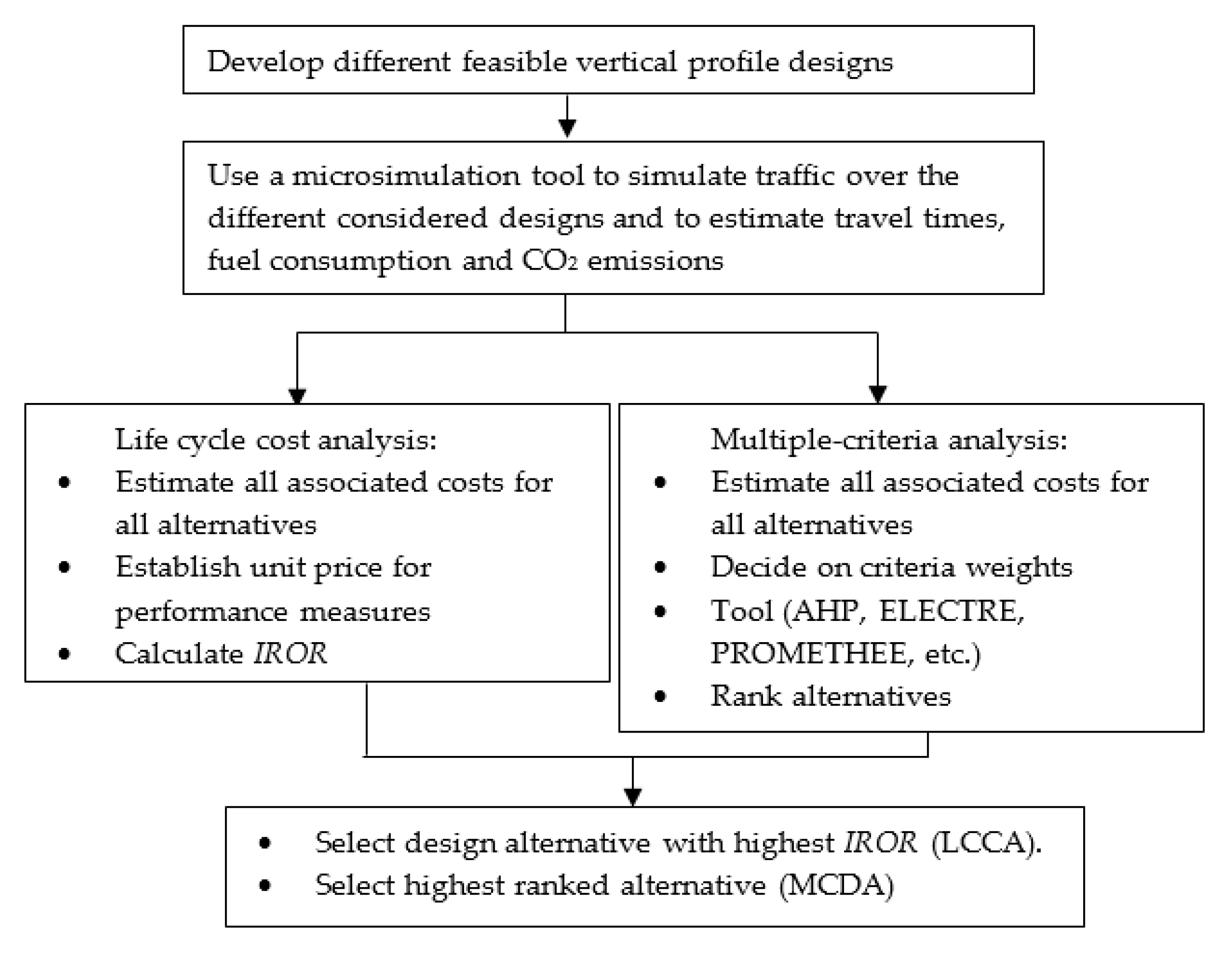
3. Proposed Evaluation Procedure

Figure 1 shows the proposed longitudinal profile road design procedure. It is up to the geometric road designer to come up with alternatives regarding the vertical slope choice. Of course, on level terrains, there might be only one alternative—the proposed procedure is not applicable in that case. However, in rolling and mountainous terrains, the designer could propose several alternatives. Usually, in these types of situations, the designer chooses a low design speed in order to minimize the initial cost of the roadway. With a low design speed value, a larger maximum vertical slope is allowed in geometric design specifications. The designer would then follow the terrain slopes, provided they do not exceed this maximum allowable design slope for the studied highway. Sometimes, when the distance is long and the slope is high, the designer keeps the maximum design slope and adds an additional lane for slow vehicles. Even in steep downhill cases, the designer leaves the grade at its maximum allowable value and designs escape ramps to be used by trucks with braking problems. Therefore, the proposed procedure does not oversimplify the existing geometric design process. In fact, the designer should come up with the slopes and vertical curves’ values that verify the chosen design speed (usually low value for tough terrains for the sole purpose of minimizing initial construction cost). In fact, the designer is accustomed to coming up with one solution without verifying that it is the “optimal” solution. It is therefore recommended that the designer investigate at least three feasible alternatives when designing the vertical profile in rolling and mountainous terrains rather than just accepting the profile that closely follows the existing terrain and uses the maximum allowable grade. It is recommended that the designer propose alternatives with smaller feasible vertical grades (i.e., consider an increase in the design speed even in rolling and mountainous terrains). Once the alternatives are established, the designer should estimate all involved costs for all alternatives. Types of costs to be estimated include excavation (this cost depends greatly on the soil type to be excavated), transportation of fill material (in case of filling to reduce a grade), construction of additional lanes or escape ramps for trucks (for the base alternative), etc. Life cycle cost analysis for selecting a project is a comparative study. This means that costs associated with all alternatives can be eliminated from the comparison. For example, costs associated with environmental impacts due to the road construction are thought to be similar for all alternatives. The same applies for maintenance costs. Even though the authors believe that degradation will decrease with grade reduction, there are no published studies affirming this hypothesis. The authors know that slower heavy loads will induce higher strains in the hot-mix asphalt layer, which accelerates pavement degradation (fatigue and rutting). Once all the costs are estimated, the designer should use a traffic microsimuation tool to reasonably estimate travel times, fuel consumption, and CO₂ emissions. If the decision maker can estimate other measures of effectiveness (such as accidents and emission of other pollutants as NO_x, SO_x, PM₁₀, and PM₅) between the proposed alternatives, then he/she should include them in the analysis.

Results of the microsimulation tool are then used as input for two different types of analysis, depending on the decision maker’s preference. Many agencies prefer the use of LCCA to select the alternative with the best dollar net revenues. For this type of analysis, all costs associated with the alternatives during the analysis period must be estimated. To estimate the benefits of one alternative over another, unit prices for user time, fuel, and CO₂ emissions are established. The benefits are the saved user costs associated with one alternative versus another multiplied by the considered unit cost. Other criteria, such as accidents (crashes, injuries, deaths) could be taken into account if they can be estimated within a certain level of reliability. Once the costs and benefits of one project versus another are all established in dollar values for the whole analysis period, an economic indicator, as discussed above, can be calculated to select the best cost-effective alternative. For this study, the IROR is used.

Agencies that prefer not to use LCCA, given the difficulties in choosing an appropriate analysis period, an appropriate discount rate, and/or during the conversion process of performance measures into monetary value, can use any MCDA tool to compare alternatives. For this type of analysis, the costs associated with the different alternatives should also be estimated. The advantage of these types of methods is that the performance measures are used as is and do not need to be converted into a monetary value. The disadvantage of these methods is that the result depends on the chosen weight for the different criteria, which various individuals perceive differently. For instance, a businessperson may perceive cost to be the most important criterion, while an environmentalist may perceive CO₂ emissions and fuel consumption to be most important. For this reason, a sensitivity analysis is always recommended, wherein the weights are changed to study the effects on the final selection.

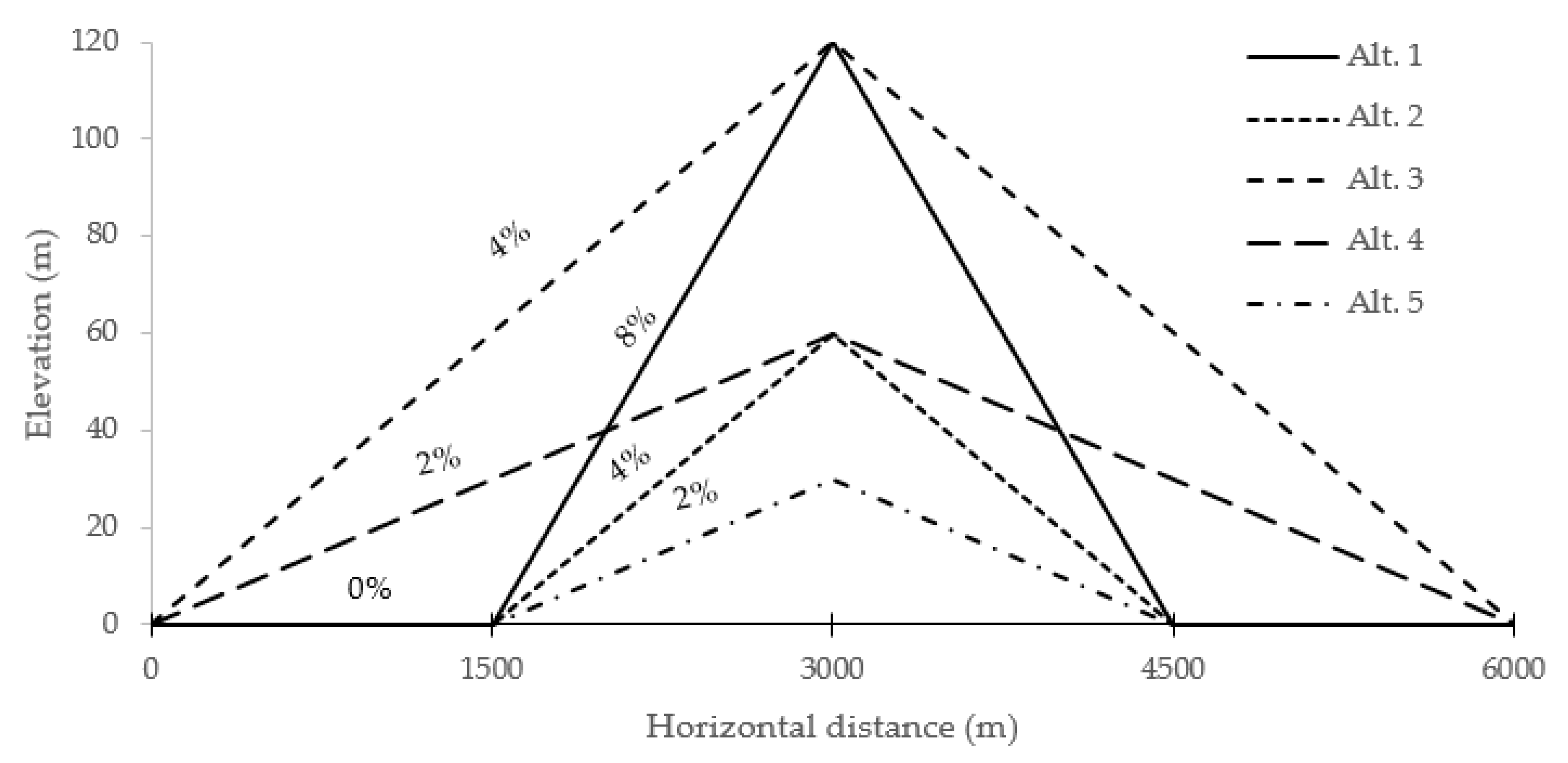
4. Case Study: Description, Results, and Discussion

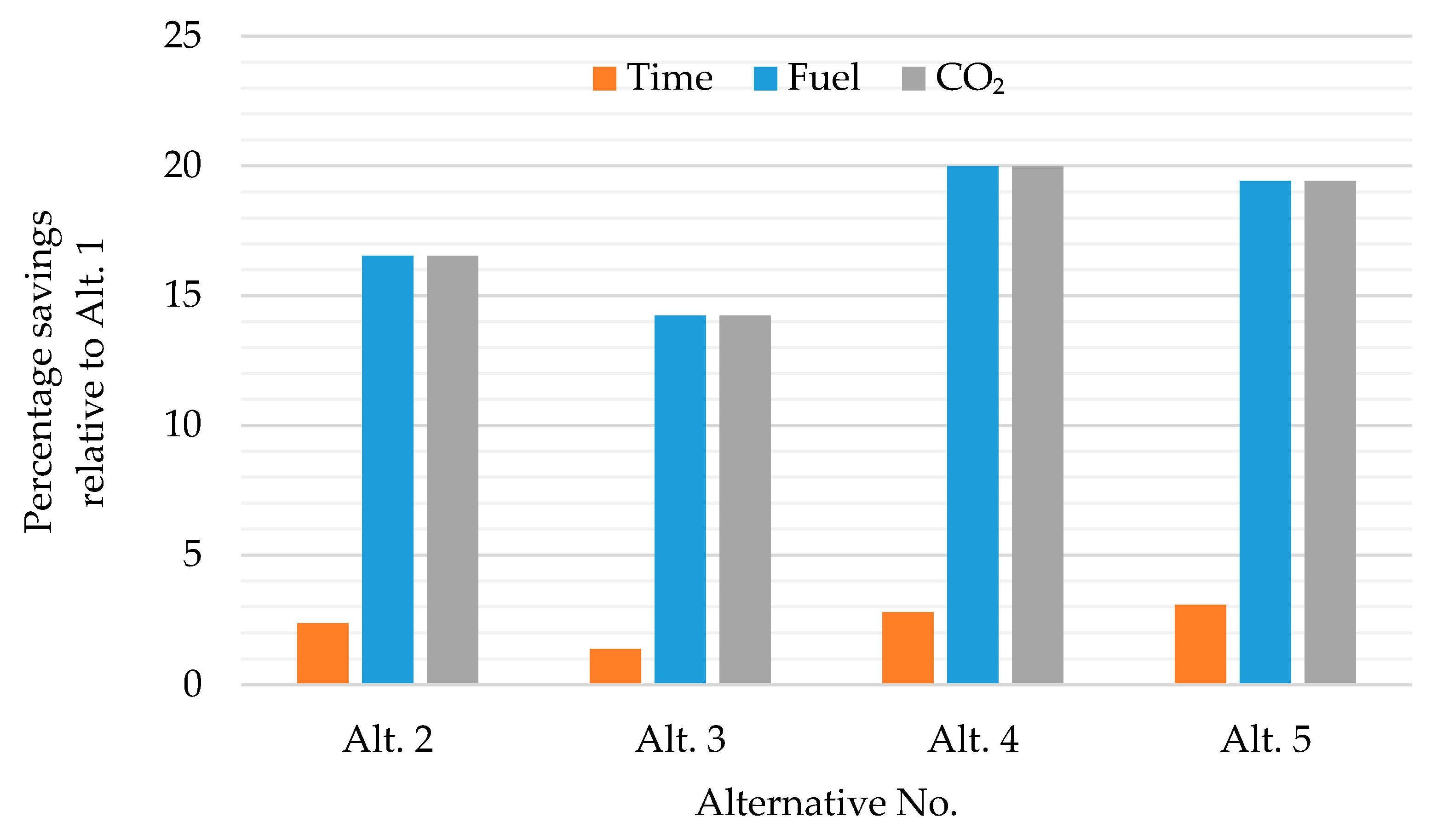
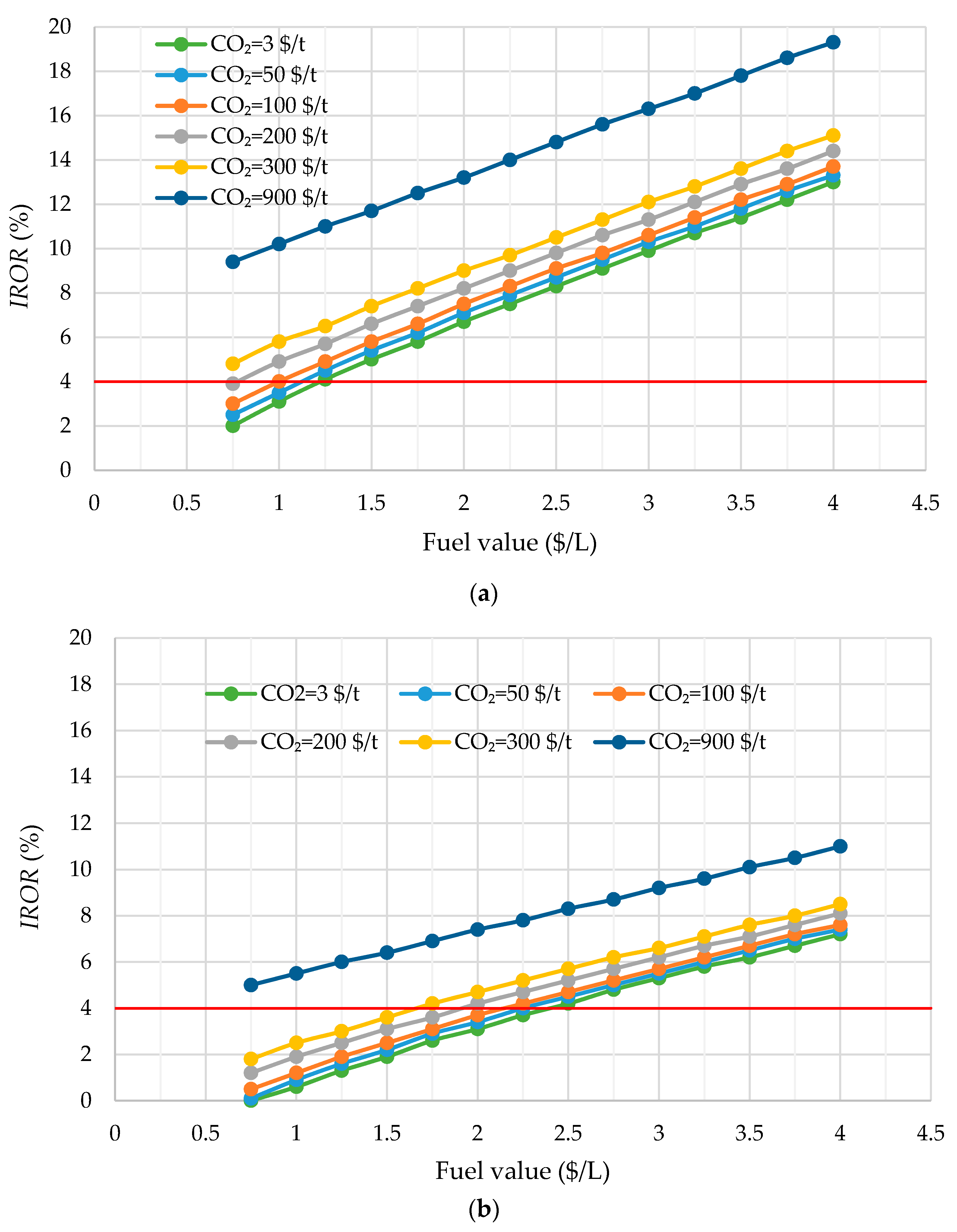
To test the proposed procedure, a case study was considered. The case study was adopted from Prassas and Roess’ Engineering Economic and Finance for Transportation Infrastructure [24]. In their example, Prassas and Roess used LCCA to evaluate the option of reducing the severity of an existing grade of a rural road. The difference in this study is that the length of the highway section was taken equal to 6 km (double of that used in the example by Prassas and Roess) so that the alternatives would have the same start and end elevations. All alternatives were assumed as new designs with alternative one being the design that followed the existing terrain. Two more designs were also considered in addition to the three treated by Prassas and Roess. Therefore, five different alternatives (Alt. 1 to Alt. 5) were studied, as shown in Figure 2. Alt. 1 is the basis design with minimum earthwork costs. It consists of two 1.5-km leveled sections and two 1.5-km 8% sections (one uphill and one downhill). Alt. 2 would make the 8% sections 4% sections instead. Alt. 3 makes the whole 6-km road a 4% grade (3 km uphill and 3 km downhill). Alt. 4 consists of making the whole 6-km road a 2% grade (3 km uphill and 3 km downhill). Alt. 5 keeps the 0% grade sections and brings the uphill and downhill sections to 2%. Obviously, in a real-life situation, using a 0% grade is not recommended (grade should be ≥ 0.3% for drainage purposes). However, the case study is used to validate the procedure and the authors believe that the results will not be affected by such an assumption. In addition, the vertical curves were not considered since they will not affect the measures of effectiveness (travel time, fuel consumption, and CO₂ emissions) results.

INTEGRATION was then used to simulate traffic over the five considered cases. Traffic characteristics were kept the same for all alternatives in order to study the effect of grade on performance (travel time, fuel consumption, and CO₂ emissions).

Table 1. Traffic characteristics used for the case study.

Characteristics	Value
Average annual daily traffic	2000
Percentage of trucks	15%
Directional distribution	50/50
Proportions of daily traffic occurring during the peak hour	15%
Free flow speed	120 km/h
Speed at capacity	90 km/h
Jam density	160 veh./km/lane
Saturation flow rate	1800 veh./h/lane

shows the main assumptions used for the traffic simulations. The infrastructure was modeled as a 2 × 2 highway. Simulating uphill and downhill movements is very important, as many researchers think that consuming more driving fuel uphill would be compensated for by consuming less fuel when driving downhill, and hence designers should always follow the terrain grade. Results of the simulations can be used to show whether this argument is valid. The modeled vehicles were a car with a mass of 1550 kg and a power of 132 kW and a truck with a total mass of 27,500 kg and a power of 354 kW. These represent typical characteristics for cars and trucks in the U.S. However, the used vehicles do not have the modern engines that cut the injection when driving downhill since the available software does not model engine cut offs, at this time. This feature could be added in future versions of the software.

Figure 3a–c shows the per year travel time, fuel consumption, and CO₂ emissions for all treated alternatives as predicted by INTEGRATION. In terms of travel time, all the alternatives resulted in similar values for cars of around 324 kilo-vehicles times hour (kveh. × h) per year. This is explained by the average travel speed of around 115 km/h, which did not differ as a function of grade. Average travel speed for trucks, on the other hand, was found to differ as a function of grade, with a value of 58.2 km/h at 8% uphill, 86.2 km/h at 4% uphill, 101 km/h at 2% uphill, while the average truck speed traveling on leveled grade or downhill was around 113 km/h. This difference in travel speed going downhill or uphill explains the difference in total travel time per year for trucks for the different alternatives. The total travel time per year for trucks predicted for Alt. 1 was 72.5 kveh. × h and decreased to 60.6 kveh. × h for Alt. 5.

For fuel consumption, the values predicted for cars and trucks differed significantly between the alternatives, with Alt.1 being the worst case. Cars were predicted to consume 4.2 million liters (ML) of fuel per year when traveling on the road as designed for Alt.1. This number decreased to 3.4 ML for Alt. 2 and 3.2 ML for Alt. 5. For trucks, a similar trend was observed, as 6.1 ML of fuel per year would be consumed by trucks traveling on the road as designed for Alt.1, with a decrease in consumption to 5.1 ML per year for Alt. 2. This result is mainly due to the dependency of fuel consumption on the grade value. For cars, the average fuel consumption on the level road was found to be 8.5 L/100 km, increased to 23.4 L/100 km uphill on a grade of 8% (an increase of about 174%), and decreased to 4.3 L/100 km downhill on a grade of 8% (a decrease of about 49%). Therefore, the notion that going downhill compensates for the extra fuel consumed going uphill proves not to be accurate, as the percentage increase going uphill is much more than the percentage decrease going downhill (about 3.5 times). For trucks, the average fuel consumption on the level road was found to be 77.6 L/100 km, increased to 197.4 L/100 km uphill on a grade of 8% (an increase of about 154%), and decreased to 14.5 L/100 km downhill on a grade of 8% (a decrease of about 81%). This confirms that fuel consumption does not vary linearly with grade value. The rate of increase in fuel consumption going from a negative grade (downhill) to a level road (0%) is much smaller than the rate of increase going from a level road to a positive grade (uphill).

As expected, the CO₂ emission trend is similar to that for fuel consumption given that CO₂ emissions are equal to a constant multiplied by the fuel consumption. The constant used varies depending on the vehicle type. Cars (trucks) traveling on a road as designed for Alt. 1 are expected to emit 9.7 (14.1) kilotons (kt) of CO₂ per year. These numbers decrease to 7.6 kt (11.6 kt) per year for cars (trucks) traveling on a road designed for Alt. 5.

To conclude this discussion, a comparison in performance measures of all alternatives relative to Alt. 1 was established, as shown in Figure 4. In terms of travel time, Alt. 1 was found to be outperformed by a value ranging between 1.4% (Alt. 3) and 3% (Alt. 5). For fuel consumption and CO₂ emissions, Alt. 3 outperformed Alt. 1 by 14.2%, while Alt. 4 reached savings as high as 20%.

In summary, all alternatives outperformed Alt. 1 in terms of travel time, fuel consumption, and CO₂ emissions. The next question is whether these savings outweigh the increase in cost associated with earthwork needed to bring the road level to the proposed values for each alternative. This question can be answered based on the results of the LCCA and MCDA tool presented in the following sections.

4.1. LCCA Results

In order to perform LCCA, different assumptions about construction- and user-related costs must be made.

Table 2. Assumed earthwork and user costs.

Item	Cost
Earthwork cost Alt. 1 (M$)	4
Earthwork cost Alt. 2 (M$)	60
Earthwork cost Alt. 3 (M$)	44
Earthwork cost Alt. 4 (M$)	88
Earthwork cost Alt. 5 (M$)	120
Value of travel time ($/(veh. × h), cars	30
Value of travel time ($/(veh. × h), trucks	56
Value of fuel ($/L)	0.75–4
Value of CO2 emissions ($/t)	3, 50, 100, 200, 300, 900

summarizes the assumptions used in this study. The earthwork costs were calculated based on quantity of cut in m³ and the average unit price for regular excavation used in the State of Virginia (20 $/m³). It was assumed that the cut material is of acceptable quality to be used in the fill areas for Alt. 3 and Alt. 4. The fuel cost per liter and the CO₂ cost per ton were varied, as shown in the table, in order to study the sensitivity of these values on the calculated IROR. The analysis period was taken to be equal to 50 years. Alt. 1 was taken as the basis alternative since it is the common geometric design and the least expensive alternative.

Figure 5a shows the variation of the calculated IROR as a function of fuel value for different prices of CO₂ emissions for Alt. 2 as compared to Alt. 1. The CO₂ emissions prices included the lowest (3 $/t) and highest (900 $/t) published values as reported by Nocera et al. [11]. If a 4% discount rate were assumed to be the minimum attractive rate of return, then Alt. 2 would be preferred over Alt.1 for a fuel value higher than 1.25 $/L, 1.12 $/L, 1.0 $/L, 0.76 $/L, 0.55 $/L, and 0 $/L for CO₂ emission prices per ton of $3, $50, $100, $200, $300, and $900, respectively. The 0.75 $/L represents the approximate current average sale price of fuel (diesel and gasoline) in the U.S. The authors believe that the value of fuel is much more than its sale price and should include the concept of sustainability, since a liter saved today would be available for use by future generations. Using a value of 4 $/L results in IROR values greater than 13%. Therefore, given these results, Alt. 2 is preferred over Alt. 1.

Figure 5b shows the variation of the calculated IROR as a function of fuel value for different prices of CO₂ emissions for the most costly alternative (Alt. 5) as compared to Alt. 1. The decision to select this high-priced alternative over Alt. 1 starts for fuel prices of about 2.3 $/L. Therefore, the decision to select even this high-cost alternative over Alt. 1 is highly recommended, especially given that other criteria that add to the benefits of this alternative were not considered. These include a reduction in fatal crashes, injuries, and physical damage to vehicles during accidents. It is known that the probability of accidents on 8% grades is higher than the probability at lower grades for driving in both directions (upgrade and downgrade). At high grades, trucks create moving bottlenecks that result in different vehicle speeds along the roadway. This speed differential causes higher crash rates. Driving downhill on an 8% grade increases the probability of truck braking mechanism failures. The addition of supplementary lanes for trucks driving upgrade and the construction of escape ramps for trucks driving downgrade would increase the cost of the base design. These additional costs and benefits were not considered in this case study to make it simpler and to show that the alternatives are more attractive than the base solution even when ignoring these parameters.

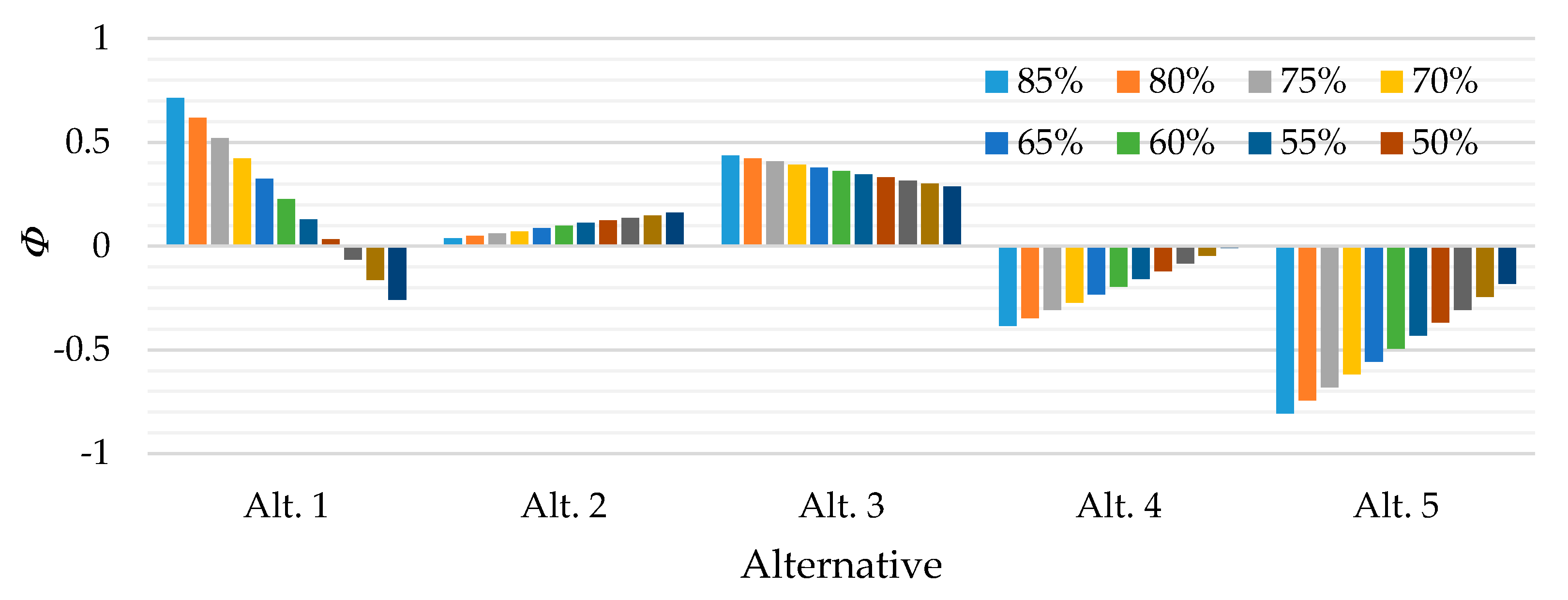
4.2. MCDA Tool Results

PROMETHEE was used to rank the proposed alternatives for different scenarios. The scenarios correspond to different weights attributed to the Cost criterion. The weight of the “Time” criterion was kept constant at 5%, while the weight for the Cost criterion was varied from 35% to 85%, which means that the weights for the “Fuel” and “CO₂” criteria were equally varied from 5% to 30%.

Table 3. Performance table as used with PROMETHEE.

	Cost (M$)	Fuel per Year (kL)	CO2 per Year (t)	Time per Year (kveh. × h)
Alt. 1	4	10,300	23,800	396.4
Alt. 2	60	8500	19,900	387.1
Alt. 3	44	8700	20,400	391.0
Alt. 4	88	8200	19,100	385.3
Alt. 5	120	8200	19,200	384.2
Indifference threshold (q)	4	600	1600	3.6
Preference threshold (p)	10	1600	4000	9.6
Weight	50–300	5–30	5–30	5

shows the performance table as used with PROMETHEE. The indifference and preference thresholds were set as recommended by the software, with the exception of the Cost criterion, where values of 4 and 10 M$ were used as thresholds to ensure a strict preference for Alt. 1 with respect to all other alternatives for this criterion. In Table 3, the green values show the best performing alternative with respect to a given criterion, while the red values show the worst preforming alternative.

Figure 6 shows the calculated net outranking flow, Φ, for all the alternatives for all considered scenarios. For a given scenario, the alternative with the highest calculated Φ is the first ranked alternative. Therefore, when the weight of the Cost criterion is higher than 70%, Alt. 1 is ranked first, followed by Alt. 3, then Alt. 2. For a Cost criterion of 65%, Alt. 3 becomes the highest ranked alternative followed by Alt. 1. Alt. 1 loses the second place to Alt. 2 when the weight of the Cost criterion is 50%. At a Cost weight of 40%, Alt.1 loses the third place to Alt. 4. At a Cost weight of 35% and lower, Alt. 1 becomes the worst ranked alternative. These results indicate that the least cost alternative is ranked first only for the scenarios in which the decision maker considers cost to be the most important criterion with a weight over 65%. This seldom happens in real-life situations, as decision makers should not consider one criterion with a weight higher than the total weights of the other considered criteria. In addition, and as discussed in the LCCA section of the paper, if safety (based on the number of crashes) were added as a criterion, then the ranking of Alt. 1 would further decrease.

5. Conclusions

With the worldwide movement towards sustainability, it is time for transportation engineers to consider road geometric designs that minimize fuel consumption and CO₂ emissions. Geometric road designers are accustomed to following the terrain profile in rolling and mountainous areas, considering only minimizing the initial cost of the road. However, on steep grades, cars and trucks emit more CO₂ and consume more fuel. Therefore, it is recommended that several feasible alternatives with different reduced slopes be included in the initial design of the vertical profile of roads. The designer should then use a traffic simulation tool to simulate the traffic that will be using the designed road to estimate the performance measures for the different alternatives. Once the performance measures are estimated, the designer can use either LCCA or an MCDA tool to select the “optimal” alternative. The proposed procedure was tested with a case study and the findings led to the following conclusions:

• The least cost alternative with the lowest required earthwork may not be the “optimal” design.
• As compared to a leveled road (0% grade), the rate of car and truck fuel consumption and CO₂ emissions is much higher when going uphill than when going downhill. Therefore, the idea that excess fuel consumed uphill is compensated by lesser fuel consumed downhill is inaccurate.
• Currently, vertical profiles of roads are the role of a geometric designer who is an expert on surveying and geometric road properties. This study recommends that transportation engineers consider a project from all perspectives (planning, design, management, etc.) and understand concepts related to traffic engineering and management.
• A design software could be developed to help the analysis described in this paper. The input to such a software is the associated costs for all alternatives (excavation, filling, transportation, materials, extra lane construction, etc.) as well as the measures of performances predicted for each alternative. The software output would be the LCCA indicators and/or the ranking of the different alternatives using any MCDA tool. Different types of uncertainties could be added to the software analysis tool.

References

1. Intergovernmental Panel on Climate Change. Climate Change 2014: Synthesis Report; Contribution of Working Groups I, II and III to the Fifth Assessment Report of the Intergovernmental Panel on Climate Change; Core Writing Team, Pachauri, R.K., Meyer, L.A., Eds.; IPCC: Geneva, Switzerland, 2015; p. 151. [Google Scholar]
2. United States Environmental Protection Agency. Inventory of U.S. Greenhouse Gas Emissions and Sinks: 1990–2017; EPA Report No. EPA 430-P-19-001; United States Environmental Protection Agency: Washington, DC, USA, 2019; p. 669.
3. Davis, S.C.; Boundy, R.G. Transportation Energy Data Book, 37th ed. Available online: https://info.ornl.gov/sites/publications/Files/Pub116893.pdf (accessed on 12 December 2019).
4. Zaniewski, J.P.; Butler, B.C.; Cunningham, G.; Elkins, G.E.; Paggi, M.S.; Machemehl, R. Vehicle Operating Costs, Fuel Consumption, and Pavement Type Condition Factors; FHWA/PL/82/00; FHWA, U.S. Department of Transportation: Washington, DC, USA, 1982.
5. Klaubert, E.C. Highway Effects on Vehicle Performance; FHWA-RD-00-164; FHWA, U.S. Department of Transportation: Washington, DC, USA, 2001.
6. Park, S.; Rakha, H. Energy and environmental impacts of roadway grades. Transp. Res. Rec. J. Transp. Res. Board 2006, 1987, 148–160. [Google Scholar] [CrossRef]
7. Chatti, K.; Zaabar, I. Estimating the Effects of Pavement Condition on Vehicle Operating Costs; NCHRP Report 720; Transportation Research Board: Washington, DC, USA, 2012. [Google Scholar]
8. Kang, M.W.; Shariat, S.; Jha, M.K. New highway geometric design methods for minimizing vehicular fuel consumption and improving safety. Transp. Res. C 2013, 31, 99–111. [Google Scholar] [CrossRef]
9. Loulizi, A.; Rakha, H.; Bichiou, Y. Quantifying grade effects on vehicle fuel consumption for use in sustainable highway design. Int. J. Sustain. Transp. 2018, 12, 441–451. [Google Scholar] [CrossRef]
10. Boriboonsomsin, K.; Barth, M. Impacts of road grade on fuel consumption and carbon dioxide emissions evidenced by use of advanced navigation systems. Transp. Res. Rec. J. Transp. Res. Board 2009, 2139, 21–30. [Google Scholar] [CrossRef]
11. Nocera, S.; Galati, O.I.; Cavallaro, F. On the Uncertainty in the Economic Valuation of Carbon Emissions from Transport. J. Transp. Econ. Policy 2018, 52, 68–94. [Google Scholar]
12. Saaty, T.L. The Analytic Hierarchy Process: Planning, Priority Setting, Resource Allocation; McGraw-Hill International Book Co.: New York, NY, USA, 1980. [Google Scholar]
13. Roy, B. Classement et choix en présence de points de vue multiples (la méthode ELECTRE). La Rev. D’Inform. Rech. Opérationelle (RIRO) 1968, 2, 57–75. [Google Scholar]
14. Brans, J.P.; Mareschal, P. Promethee Methods, Multiple Criteria Decision Analysis: State of the Art Surveys; Springer Sciences: Boston, MA, USA, 2005; Chapter 5; pp. 163–195. [Google Scholar]
15. Brans, J.P. L’Ingénierie de la Décision—Elaboration D’instruments D’aide à La Décision—Méthode PROMETHEE; Université Laval, Colloque d’aide à la décision: Quebec, QC, Canada, 1982; pp. 183–213. [Google Scholar]
16. Brans, J.P.; Mareschal, B. The Promcalc and Gaia decision-support system for multicriteria decision aid. Decis. Support Syst. 1994, 12, 297–310. [Google Scholar] [CrossRef]
17. Van Aerde, M.; Yagar, S. Dynamic Integrated Freeway/Traffic Signal Networks: A Routeing-Based Modelling Approach. Transp. Res. 1988, 22, 445–453. [Google Scholar] [CrossRef]
18. Van Aerde, M.; Rakha, H. INTEGRATION © Release 2.40 for Windows: User’s Guide—Volume I: Fundamental Model Features; M. Van Aerde & Assoc., Ltd.: Blacksburg, VA, USA, 2013. [Google Scholar]
19. Rakha, H.; Pasumarthy, P.; Adjerid, S. A Simplified Behavioral Vehicle Longitudinal Motion Model. Transp. Lett. Int. J. Transp. Res. 2009, 1, 95–110. [Google Scholar] [CrossRef]
20. Van Aerde, M.; Rakha, H. Multivariate calibration of single regime speed-flow-density relationships [road traffic management]. In Proceedings of the Vehicle Navigation and Information Systems Conference, in conjunction with the Pacific Rim TransTech Conference: 6th International VNIS: A Ride into the Future, Seattle, WA, USA, 30 July–2 August 1995. [Google Scholar]
21. Rakha, H.; Ahn, K.; Moran, K.; Saerens, B.; Van Den Bulck, E. Virginia Tech comprehensive power-based fuel consumption model: Model development and testing. Transp. Res. D 2011, 16, 492–503. [Google Scholar] [CrossRef]
22. Guo, J.X.; Tan, X.; Gu, B.; Qu, X. The impacts of uncertainties on the carbon mitigation design: Perspective from abatement cost and emission rate. J. Clean. Prod. 2019, 232, 213–223. [Google Scholar] [CrossRef]
23. Xu, Z.; Elomri, A.; Pokharel, S.; Zhang, Q.; Ming, X.G.; Liu, W. Global reverse supply chain design for solid waste recycling under uncertainties and carbon emission constraint. Waste Manag. 2017, 64, 358–370. [Google Scholar] [CrossRef]
24. Prassas, E.S.; Roess, R.P. Engineering Economics and Finance for Transportation Infrastructure; Springer: Berlin, Germany, 2013. [Google Scholar]
Figure 1. Proposed procedure.
Sustainability 11 07127 g001
Figure 2. Vertical grade design alternatives.
Sustainability 11 07127 g002
Figure 3. Measures of performances for the different alternatives: (a) travel time; (b) fuel; (c) CO2.
Sustainability 11 07127 g003
Figure 4. Percentage savings in performances for alternatives relative to Alt. 1.
Sustainability 11 07127 g004
Figure 5. Internal rate of return (IROR) as a function of fuel and CO2 prices for (a) Alt. 2 vs. Alt. 1; (b) Alt. 5 vs. Alt. 1.
Sustainability 11 07127 g005
Figure 6. Calculated net outranking flow for the different alternatives for the various considered Cost weights.
Sustainability 11 07127 g006