Spatio-Temporal Variation of Heavy Metal Pollution during Accidents: A Case Study of the Heshangshan Protected Water Area, China

Abstract

Recently, water environmental accidents have occasionally occurred which have had wide-ranging influences, long durations and are difficult to deal with. The development of the social economy, the acceleration of industrialization, the huge discharge of industrial wastewater and the occasional occurrence of ship transportation accidents pose serious threats to the water quality of water inlets and protected water areas. This article applied the two-dimensional water quality model, used a GIS platform and FORTRAN language, and predicted spatio-temporal variations of the iron concentration during a water pollution accident. This research selected the water inlet of Heshangshan Water Plant and the Heshangshan protected water area as the research objective, and assumed a water pollution event had occurred. It was suggested that we should take corresponding emergency measures and relevant solutions to deal with the bad effects of water pollution accidents. The processes mainly included the selection of the study area, the determination of the equation to be used, parameters determination, as well as the identification of the accident scenario and source. The durations of the iron concentration exceeding the standard at the water inlet were 12–18 min and in the protected water area were 16–36 min in four water periods after the accident. In addition, the durations taken for the iron concentration to decrease to the background value in the protected water area were 18–38 min after the accident in four water periods in the accident scenario. Relevant departments should take some contingency measures to avoid fetching water from the intake after the accident within 40 min after the accident and the relevant staff can cancel the warning 40 min after the accident.

1. Introduction

Considering that 80% of human diseases are related to unsafe drinking water, according to the World Health Organization [1,2,3], drinking water is a major issue that can affect human health [4,5]. In consequence, drinking water safety has attracted the attention of many countries and has become a global strategic issue [6,7,8]. Water inlets are the points where water plants draw water from and protected water areas are the source of drinking water. Therefore, it is indispensable to ensure the water quality safety of water inlets and protected water areas. This paper contributes to producing knowledge in order to achieve SDG 6 (SDG 6 is clean water and sanitation, which aims to ensure water and sanitation for all and to achieve the sustainable management of water and sanitation) building on the previous literature on water and SDG 6 in its different dimensions [9,10,11]. Nowadays, heavy metal pollution has become one of the most important factors threatening water safety [12,13]. When heavy metals enter into the environment, the impacts are serious, long-term and difficult to eliminate [14]. Moreover, heavy metals tend to be highly toxic, easily enriched by organisms [15,16,17], and difficult to metabolize, which poses a serious threat to human life. As a result, it is important to study the spatio-temporal variation of heavy metals, which can supply decision-making for contingency planning. The dam break of Zijin Mining in 2010 was a significant environmental pollution event. The ketonic acid water leakage accident occurred in the Zijinshan Copper Mine Wet Process Plant of Fujian Province. The accident caused serious heavy metal pollution in the waters of the Tingjiang River. As the factory underreported the accident for nine days, none of the local residents dared to use the tap water. In 2011, there was a water pollution event in the Fujiang River of the Yangtze River Basin [18]. Heavy rain fell on the upper reaches of the Fujiang River and the debris flow brought the tailings of an electrolyzed manganese plant in Aba Autonomous Prefecture into the Fujiang River [19], which affected the water quality of the water inlet and the daily life of about 500,000 residents. A cadmium pollution accident occurred in the Longjiang River of Guangxi Province in 2012 [20], which influenced about 300 km of river and the water-drinking of residents along the river. The Three Gorges Project (TGP) is the largest water conservancy project in the world, and its reservoir area involves 30 million people [21,22]. Therefore, there are numerous water inlets of drinking water plants and protected water areas in the Three Gorges Reservoir Area, so the water quality safety of it is an important prerequisite for social and economic development. Predicting the concentration of heavy metals in an accident scenario is an important way to realize the safety warning and emergency response of the water inlet and the protected water area. It is particularly important to set up accident scenarios and carry out the prediction and analysis of the concentration of typical heavy metal pollutants with time and space in the Three Gorges Reservoir Area.

Many countries worldwide attach great importance to the prediction of pollution accidents, which is conducive to the formulation of scientific and reasonable emergency plans. The dispersion–advection equation was solved analytically and numerically and used to simulate the concentration of benzene and nitrobenzene in the Songhua River after the accident by Fu et al. (2008). The arrival time of the pollutant wave, the peak concentrations and the end of the pollutant wave at Harbin and along the river were predicted [23]. Wang et al. (2007) studied the chemical distribution of arsenic, iron, lead, antimony, zinc and other elements in stream sediments after the cadmium pollution accident in the Longjiang River. In order to better understand the toxicity of these pollutants and evaluate their ecological risks, the pollution levels of heavy metals in sediments were evaluated by principal component analysis (PCA) and geological accumulation index (I-geo). The results provide a good basis for the determination of heavy metal pollution in sediments [24]. The canal bridge is considered to be a typical location for pollution accidents, and the truck’s response, road conditions and human response are the main factors leading to sudden pollution accidents. Therefore, Tang et al. (2015) established a Bayesian network model to calculate the risks of water pollution and used MIKE 11 to simulate the fluid field and contaminant transport process. According to the calculation results, emergency countermeasures such as water diversion and water gate management were proposed [25]. Using techniques such as GIS, professor Hind Mohammad assessed drought conditions in the Yarmouk Basin (YB) in Northern Jordan, showing that drought periods are frequent and irregular as drought intensity and frequency change [26]. Nevertheless, there is still a limitation. Much research has focused on rivers and lakes, while few of them have concentrated on the prediction of the variation of pollutant concentration at water inlets and in protected water areas during water pollution accidents. However, predictions of the spatio-temporal variation of pollutant concentration at water inlets and in the protected water areas in accident scenarios contribute to the formulation of emergency plans and rapid response. Because the water plant takes water from the water inlet and supplies water to residents, the water quality of the water inlet is directly related to residents’ daily life and body health. Therefore, it is necessary to systematically carry out relevant research and proceed with the prediction of the water inlet and the protected water area in accident scenarios, so as to provide technical guidance and support for the water quality safety of domestic drinking water.

Based on the existing model, spatio-temporal variations of the pollutants of the water inlet and the protected water area in the accident scenario were predicted by using a GIS platform and FORTRAN language. Moreover, the durations of the iron concentration exceeding the standard at the water inlet, and the durations of the iron concentration exceeding the standard as well as spatio-temporal variations of the iron concentration in the protected water area were obtained. This will give a reference for relative research in method and provide strategic suggestions for decision makers in the prevention and treatment of water pollution accidents.

2. Materials and Methodology

2.1. Study Area

In this study, the Heshangshan protected water area was selected as the representative of the Three Gorges Reservoir Area (TGRA). It is the largest protected water area in the TGRA. In addition, the protected water area is the drinking water source of nearly one million residents in Chongqing City, which is the main city in the TGRA. The study area spanned 106°31′40″ E–106°32′25″ E, 29°30′43″ N–29°31′22″ N and covered 432 km². It belongs to Jiulongpo District, which is located in the southwest of the main city of Chongqing City. The District borders Yuzhong District, Shapingba District, Jiangjin District as well as Bishan County, and faces Nan’an District as well as Banan District across the river. The longest distance from north to south is 36.12 km, and the width from east to west was 30.4 km. The terrain map of Heshangshan is shown in Figure 1. The Heshangshan protected water area was the water intake area of Heshangshan water plant, and the plant withdrew 200,000 t/d of water from the study area and serviced 980,000 residents in Daping, Yangjiaping, Shiqiaopu and Zhongliangshan areas. The water plant also provided domestic water to some areas, such as Yuzhong District and Shapingba District. The water inlet of Heshangshan (106°31′54″ E, 29°31′11″ N) was located under the Egongyan Bridge in Chongqing City, near the left bank of the river. According to water quality monitoring data, the water qualification rate of Heshangshan protected water area was about 80% in recent years, which was lower than the desired one of 95%. Pollutants beyond level III of the water quality standard (GB3838-2002) in the protected water area included iron.

According to topographic data in the study area, data collection and a field investigation were conducted to obtain the cross-section data of the Heshangshan protected water area. The GIS-based inverse distance weighting method was used to process the terrain to generate the DEM diagram of the Heshangshan protected water area, as shown in Figure 2.

2.2. Methodology

2.2.1. Governing Equation

Strictly speaking, the models of water pollution are usually three-dimensional, but the three-dimensional model can be simplified to two-dimensional, one-dimensional or even zero-dimensional according to the assumptions of the model and the actual practical requirements. In general, the protected water area in cities and towns is relatively large (for river-type drinking water sources); the depth of the river is far less than the length and width of it. It is usually considered that the distribution of pollutants in the depth direction of the river is uniform, so it can be assumed that the contaminant does not substantially diffuse in the z direction, that is, the concentration diffusion coefficient is approximately zero; and the diffusion coefficient is non-zero in the x and y directions. Therefore, this study used the two-dimensional water quality model [27,28,29].

Water quality control equations in the following conserved form were adopted without considering wind shear stress and the Coriolis force [30,31,32,33]:

$$\frac{\partial h}{\partial t}+\frac{\partial h_u}{\partial x}+\frac{\partial h_v}{\partial y}=q,$$

(1)

$$\frac{\partial h_u}{\partial t}+u\frac{\partial h_u}{\partial x}+v\frac{\partial h_u}{\partial y}=-g\frac{\partial h^2}{\partial x}-gh\frac{\partial h_b}{\partial x}-g{n}^2\frac{u\sqrt{u^2+v^2}}{h^{1/6}}+\frac{\partial }{\partial x}\left({\epsilon }_{x}h\frac{\partial u}{\partial x}\right)+\frac{\partial }{\partial y}\left({\epsilon }_{x}h\frac{\partial u}{\partial y}\right),$$

(2)

$$\frac{\partial h_v}{\partial t}+u\frac{\partial h_v}{\partial x}+v\frac{\partial h_v}{\partial y}=-g\frac{\partial h^2}{\partial x}-gh\frac{\partial h_b}{\partial y}-g{n}^2\frac{v\sqrt{u^2+v^2}}{h^{1/6}}+\frac{\partial }{\partial x}\left({\epsilon }_{y}h\frac{\partial v}{\partial x}\right)+\frac{\partial }{\partial y}\left({\epsilon }_{y}h\frac{\partial v}{\partial y}\right),$$

(3)

$$\frac{\partial h_c}{\partial t}+u\frac{\partial h_c}{\partial x}+v\frac{\partial h_c}{\partial y}=\frac{\partial }{\partial x}\left(E_x\frac{\partial h_c}{\partial x}\right)+\frac{\partial }{\partial y}\left(E_y\frac{\partial h_c}{\partial y}\right)+H\sum S_i,$$

(4)

where x and y are the longitudinal and transverse flow distances of the river; u and v are the flow velocity of the river in the x and y directions; t is time; h is the water depth; z is the water level; h_b is the river bottom elevation; c is the concentration of a pollutant in the reach; ε_x, ε_y are x, y direction of the eddy viscosity coefficient, respectively; g is the gravitational constant; E_x and E_y are the sum of the molecular diffusion coefficient, turbulent diffusion coefficient and dispersion coefficient in x and y directions, respectively; n is the roughness of the reach, and q is the interval inflow of the reach. ∑Si is the sink source term of water pollutant. (In this article, $\sum S_i=K_{1}c+S_0$ and K₁ is degradation coefficient and S₀ is foreign exchange).

2.2.2. Equation of Discrete

For Equations (1)–(4), the finite volume method was used to discretize [34]:

$${\alpha }_P {\varphi }_p={\alpha }_E{\varphi }_E+{\alpha }_w{\varphi }_W+{\alpha }_N{\varphi }_N+{\alpha }_S{\varphi }_S+b,$$

(5)

The SIMPLEC method was used for the discretization of the continuity equation and the momentum equation, and the pressure-weighted interpolation method was used for the pressure correction formula, where α was the relaxation factor of the SIMPLEC method. The discrete equations are shown in Equation (5).

The parameter values are shown in

Table 1. Discrete parameter list of equations.

	Continuity Equation	Momentum Equation	Water Quality Equation
$\varphi$	$z^{\prime }$	u v	c
${\alpha }_P$	${\alpha }_E+{\alpha }_W+{\alpha }_N+{\alpha }_S$	$({\alpha }_E+{\alpha }_W+{\alpha }_N+{\alpha }_S+{\alpha }_P^0-S_p\Delta x\Delta y)/\alpha$
${\alpha }_E$	${\overline{d}}_e{h}_e\Delta y$	$D_{e}A\left(\left|P_e\right|\right)+-⟦F_e,0⟧$
${\alpha }_w$	${\overline{d}}_w{h}_w\Delta y$	$D_{w}A\left(\left|P_w\right|\right)+-⟦F_w,0⟧$
${\alpha }_N$	${\overline{d}}_n{h}_n\Delta x$	$D_{n}A\left(\left|P_n\right|\right)+-⟦F_n,0⟧$
${\alpha }_S$	${\overline{d}}_s{h}_s\Delta x$	$D_{S}A\left(\left|P_S\right|\right)+-⟦F_S,0⟧$
$b$	$u_e^{*}{h}_e\Delta y+u_w^{*}{h}_w\Delta y-v_n^{*}{h}_n\Delta x+v_s^{*}{h}_s\Delta x+\left(h_p^0-h_p^{*}\right)\Delta x\Delta y/\Delta t+q\Delta x\Delta y$	$S_c\Delta x\Delta y+{\varphi }_p^0{\alpha }_p^0+\left(1-\alpha \right)/\alpha {\alpha }_p{u}_p^{*}$
${\alpha }_p^0$	—	$h_p^0\Delta x\Delta y/\Delta t$
$D_e$	—	${\left({\epsilon }_{x}h\right)}_e\Delta y/\Delta x$
$P_e$	—	$F_e/D_e$
$S_p$	—	$-g{n}^2\sqrt{u^2+v^2}/h^{1/3}-q$	$-KH$
$S_c$	—	$-gh\left(Z_e-Z_w\right)/\Delta x$	$c_{0}H$
$u_e^{*}$	${\left(\left(\sum {\alpha }_{nb}{u}_{nb}+b\right)/{\alpha }_P\right)}_e+{\left(gh\Delta y/{\alpha }_P\right)}_e\left(Z_P-Z_E\right)$	—	—
${\overline{d}}_e$	${\left(\Delta y/{\alpha }_P\right)}_P{\left(\delta x\right)}_{e^{+}}/{\left(\delta x\right)}_e+{\left(\Delta y/{\alpha }_p\right)}_E{\left(\delta x\right)}_{e^{-}}/{\left(\delta x\right)}_e$	—	—

.

2.3. Parameter Determination

After the water quality prediction model was confirmed, the next step was to select and determine the parameters of the water quality prediction model. The accuracy and rationality of the parameter measurement are closely related to the reliability and scientificity of the water quality prediction model. The model is often simplified by certain assumptions for its practical application. There are many factors to be determined; however, the most important ones are the transverse diffusion coefficient and the longitudinal diffusion coefficient. Nowadays, the common parameter estimation methods of the water quality prediction model mainly include the empirical formula estimation method, the data calculation method and the method of directly referring to the data verified by the predecessors. Through investigation and the reviewing of the related literature, the empirical formula method was chosen to estimate the parameters of the water quality prediction model.

2.3.1. Transverse Diffusion Coefficient

The transverse diffusion coefficient in natural water is denoted as D_y, and the following empirical formula is used for calculation [35]:

$$D_y=\alpha H{u}^{*},$$

(6)

$$u^{*}=\sqrt{gHi},$$

(7)

where H is the average water depth of the river; α is the transverse diffusion coefficient of dimension 1; u* is the friction velocity; g is the gravitational acceleration; i is the average hydraulic gradient of the river.

The value of the transverse diffusion coefficient can be seen in

Table 2. Value reference table of the transverse diffusion coefficient.

River Type	α Reference	Note
Straight rectangular open channel	0.24~0.25	-
Straight natural river course	0.1~0.2	The average is 0.15.
A natural river with gentle bend and irregular channel	0.3~0.9	Small value can be taken when the channel shrinks, larger value can be taken when it expands, and 0.6 can be taken when it is uniform
A large bend in a natural river course	$\mathsf{\alpha }=0.25{\left(\frac{u}{u^{*}}\right)}^2\left(\frac{H}{R_c}\right)\frac{1}{K^5}$	u—average velocity of section, m/s; K—Karman Constant, Preferable 0.41; Rc—The bend radius, m.

.

2.3.2. Longitudinal Diffusion Coefficient

Considering that the longitudinal dispersion coefficient is much larger than the longitudinal diffusion one, the latter coefficient is ignored when they are studied together. Empirical formulas commonly used for the river longitudinal dispersion coefficient are shown in

Table 3. Calculation method of the longitudinal dispersion coefficient.

Calculation Formula	Note
$D_x=5.93H{u}^{*}$	Elder Formula (suitable for natural rivers)
$D_x=0.01u^2{B}^2/H{u}^{*}$	Fischer Formula
$D_x=0.007{\left(B/H\right)}^{2.1}{\left(u/u^{*}\right)}^{0.7}H{u}^{*}$	Formula of the Chinese academy of hydropower sciences
$D_x=\gamma u^{*}{A}^2/H^3$	H. Liu Formula
$D_x=\left(1-\frac{u^2}{2gH}\right)0.115Q/2Bi$	Mcquivey–Keefer Formula

.

3. Spatio-Temporal Variations of Iron Concentration in the Accident Scenario

3.1. Accident Scenario

This study hypothesized the accident scenario of iron pollution occurring in the Heshangshan protected water area. When drinking water contains too much iron, people who drink it will suffer from a hypoxia symptoms, leading to cell membrane damage, mitochondria membrane damage, electron transport problems and nervous system toxicity, which can be life threatening. In addition, according to the monthly monitoring data of the Heshangshan protected water area in 2016, the iron concentration of it increased rapidly and exceeded the standard in certain months. Therefore, iron was selected as the pollutant in this research.

Since the mobile risk sources in the protected water area included freight vehicles [36,37], this study assumed that a truck with 10 t of 40% ferric chloride overturned on the right bank of the upper boundary of the protected water area, and its pollutants flowed into the water from the bank. Let T = 0 when the accident happened, and all pollutants flowed into the protected water area in 10 min, so this study conducted research and analysis on this accident scenario. It was calculated that the iron concentration entering the water body was 16 mg/L. In addition, the degradation rate constant of the iron pollutants was 0 d⁻¹.

3.2. Determination of Boundary Conditions

In the two-dimensional water quality model, the upstream flow and the downstream water level were selected as boundary conditions of it to ensure the accuracy of the results. In this research, the upstream flow was the daily flow of the Zhutuo hydrological station, and the downstream water level was the water level of the Cuntan hydrological station. Influenced by natural or man-made factors [38,39], the annual variation of flow/water level in Zhutuo hydrologic station and Cuntan hydrologic station is obvious. The trend chart for the daily flow of Zhutuo hydrological station and the water level of Cuntan hydrological station in 2016 is shown in Figure 3. For Zhutuo hydrological station, the maximum daily flow was 29,000 m³/s, which occurred in the flood period, and the minimum one was 2770 m³/s, which occurred in the dry period. For the Cuntan hydrological station, the daily maximum and minimum water levels were 182.16 m in the flood period and 160.6 m in the down period, respectively.

3.3. Predict Processes

The reason for choosing the water inlet as the research objective is as follows. The water inlet is the place from which the water plant draws water, and the iron concentration at this location is very important for the water quality of the water plant and people’s drinking water safety. The durations for the iron concentration exceeding the standard of the water inlet and the protected water area were predicted. In addition, the spatio-temporal variation of the iron concentration in the four water periods and the durations from the time of the accident to the time when the iron concentration in the protected water area dropped to the background value were predicted and analyzed. Specifically, the durations of the iron concentration exceeding the standard in the protected water area were the durations when the maximum concentration of iron in the protected water area could not meet the standard. Only when the maximum concentration of iron in the protected water area met the standard, could the protected water area meet the standard.

The following is the basic condition of iron pollution concentration prediction and the setting and selection of the source term. In this study, the background value of iron in the protected water area is 0.1 mg/L and the standard value of it is 0.3 mg/L. Moreover, the four water periods concerned were, namely, the dry period, down period, flood period and storage period. The first period is from the end of October to the end of March, the down period extends to June 10, the flood period is from June 10 to the end of September, and then the last one is extends to the end of October. In 2016, the average flows of the protected water area in the four water periods were 3330 m³/s, 5031 m³/s, 16,083 m³/s and 10,393 m³/s, and the flow rate of the four water periods increased successively. Moreover, the time step of this study was set as one minute.

4. Results and Discussion

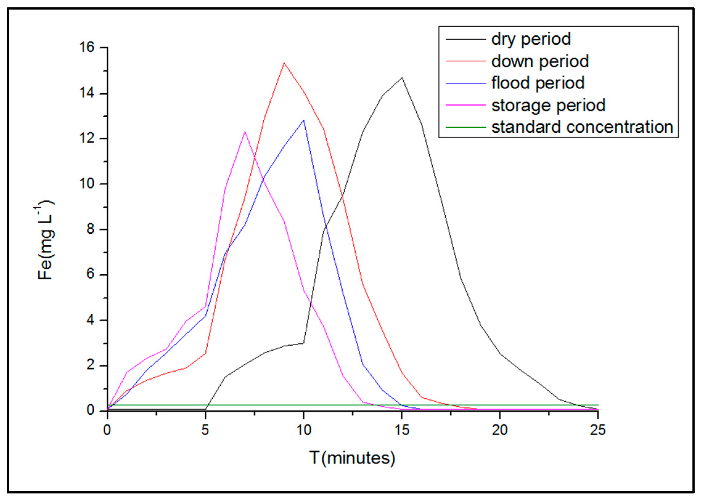
4.1. Durations of the Iron Concentration Exceeding the Standard at the Water Inlet

The velocity was an important factor to determine the diffusion rate of pollutants; the larger the velocity was, the faster the diffusion of pollutants would be, and so the sooner the pollutants reached the water inlet, the sooner the iron concentration of the water inlet met level III of water quality standards. The velocity of the water inlet was different in different water periods; in the dry period, the velocity was less than that in the down period, and the velocity of the water inlet in the down period was less than that in the flood period. Moreover, the velocity of the storage period was the largest, so the durations of the iron concentration exceeding the standard at the water inlet in the four water periods decreased successively. The starting time for pollutants to make the iron concentration of the water inlet exceed the standard in the dry period is the sixth minute after the accident, the starting time of the down period is the third minute, that of the flood period is the second minute, and the starting time in the storage period is the time of the accident. Moreover, the time when the maximum iron concentration of the water inlet occurs is the 15th minute, 10th minute, 8th minute and 5th minute after the accident in the four water periods.

The predicted results show that the polluted durations at the water inlet in the four water periods were 18 min, 15 min, 13 min, and 12 min, respectively. In conclusion, the larger the flow rate, the shorter the duration of the iron concentration exceeding the standard at the water inlet and the smaller the influence of the accident, as is shown in Figure 4.

Based on the above results, we suggest that the water inlet be closed for 20 min in the dry period and for 15 min in the remaining three water periods to ensure the safety of drinking water.

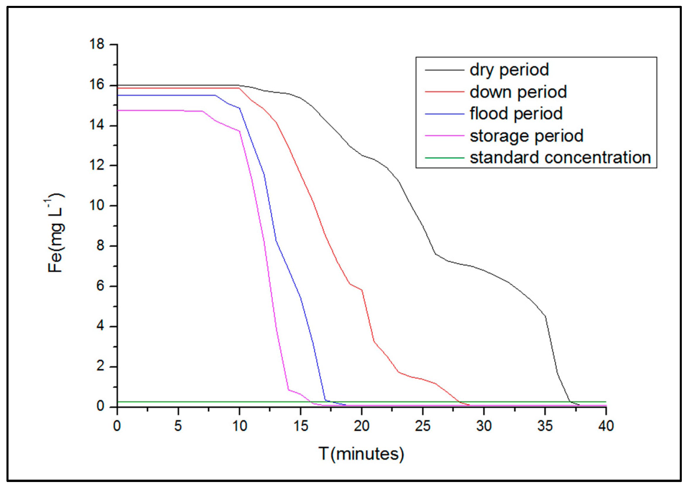
4.2. Durations of the Iron Concentration Exceeding the Standard for the Protected Water Area

The faster the velocity of water in protected water area was, the faster the diffusion rate of the pollutants was, and the shorter the duration of the iron concentration exceeding the standard in protected water area would be. In this study, the velocities of water in the four water periods decreased successively, so the length of exceeding the standard in the four water periods decreased in turn. The durations of the iron concentration exceeding the standard in the four water periods were 36 min, 28 min, 17 min and 16 min, respectively. Moreover, the maximum iron concentration in the protected water area occurred at the tenth minute after the accident.

Trends shown in Figure 5 indicate that the iron concentration in the protected water area declined over time after the accident and decreased with the increase in flow rate. In other words, the larger the flow rate was, the faster the iron concentration decreased, and the easier it was to meet the water quality standard.

Considering that the over-standard time of the iron concentration in the protected water area covered this of the water inlet, according to the national relevant regulations, it is recommended that relevant departments should take some contingency measures to avoid fetching water from the intake after the accident within 40 min in dry period, 30 min in the down period and 20 min in the remaining two water periods after the accident.

4.3. Spatio-temporal Variations of Iron Concentration in the Protected Water Area.

The spatio-temporal variation of the iron concentration in the protected water area was from the occurrence of the accident to the decrease in the iron concentration in the protected water area to the background value. In the protected water area, the water velocity and the spatio-temporal variations of the iron concentration were positively correlated. That is, the higher the flow rate, the faster the diffusion of iron pollutants in the protected water area, and the easier it was for the iron concentration in the protected water area to return to the background value.

The following are the simulation results of the dry period, down period, flood period and storage period. In this research, the abscissa axis is represented by I, J is the vertical axis; C is the concentration of the pollutant. In addition, the iron concentration of the protected water area in the four water periods could reach the background value (0.1 mg/L) with 38 min, 28 min, 18 min, and 16 min after the accident in the above scenario, respectively.

In the dry period, the maximum iron concentration in the protected water area was 16.22 mg/L, at the tenth minute after the accident. Thirty-eight min after the accident, the iron concentration decreased to the background value (Figure 6).

During the down period, the maximum iron concentration in the protected water area was 16.71 mg/L at the tenth minute after the accident. At 28 min after the accident, the iron concentration was 0.1 mg/L (Figure 7).

In the flood period, the maximum iron concentration in the protected waters was 17.95 mg/L at the same time as in the first two water periods and decreased to the background value in the eighteenth minute (Figure 8).

The maximum iron concentration was 14.77 mg/L at the fifth minute after the accident in the storage period, and the iron concentration reached 0.1 mg/L at the sixteenth minute (Figure 9).

By predicting the spatio-temporal variations of the iron concentration of the protected water area in the four water periods, it could be concluded that the higher the velocity, the less time it took for the iron concentration in the protected water area to reach the background value. At this time the water body has returned to normal state, the relevant managers can cancel the early warning.

5. Conclusions

Water pollution accidents seriously affect the safety of human life. Ensuring water safety of water inlets and the protected water area is necessary to protect people’s health. In this study, the planar two-dimensional water quality model was adopted to predict the spatio-temporal variations of the iron concentration in a certain accident scenario for the water inlet of the Heshangshan Water Plant and the Heshangshan protected water area. An iron pollution accident was assumed to have occurred in the protected water area. Then, the durations of the iron concentration exceeding the standard at the water inlet, those in the protected water area, and the spatio-temporal variations of iron concentration in the protected water area were analyzed. The conclusions were as follows.

The durations of the iron concentration exceeding the standard at the water inlet were 12–18 min in the four water periods after the accident. The relevant departments should take some contingency measures to avoid fetching water from the intake after the accident for 40 min after the accident. Furthermore, the durations of the iron concentration exceeding the standard in the protected water area were 16–36 min in the four water periods. In addition, the durations of the iron concentration decreasing to the background value in the protected water area were 18–38 min after the accident in the four water periods in the accident scenario. As a result, the relevant staff can cancel the warning 40 min after the accident.

This research can provide decision makers with fast and effective methods regarding water inlets and protected water areas. Moreover, it helps to mitigate the influence of accidents on the drinking water quality of residents after accidents. However, there are still some areas to be improved in this study. In the future, the longitudinal diffusion of pollutants and the biological damage of the water pollution accidents can be further considered [40,41].

References

1. Liu, R.Z.; Zhang, K.; Zhang, Z.J.; Borthwick, A.G.L. Water-Scale Environmental Risk Assessment of Accident Water Pollution: The Case of Laoguan River, China. J. Environ. Inform. 2018, 31, 87–96. [Google Scholar]
2. Hou, Y.; Zhang, T. Evaluation of major polluting accidents in China—Results and perspectives. J. Hazard. Mater. 2009, 168, 670–673. [Google Scholar] [CrossRef] [PubMed]
3. Kourakos, G.; Harter, T. Vectorized simulation of groundwater flow and streamline transport. Environ. Model. Softw. 2014, 52, 207–221. [Google Scholar] [CrossRef]
4. Tao, Y.; Ren, H.T.; Xia, J.X. Investigation on disposal effect of different countermeasure of sudden water pollution accident. J. Basic. Sci. Eng. 2013, 21, 203–213. [Google Scholar]
5. Ding, X.W.; Wang, S.Y.; Jiang, G.H. A simulation program on change trend of pollutant concentration under water pollution accidents and its application in Heshangshan drinking water source area. J. Clean. Prod. 2017, 167, 326–336. [Google Scholar] [CrossRef]
6. Zheng, H.Z.; Lei, X.H.; Shang, Y.Z. Sudden Water Pollution Accidents and Reservoir Emergency Operations: Impact Analysis at Danjiangkou Reservoir. Environ. Technol. 2018, 39, 787–803. [Google Scholar] [CrossRef]
7. Berg, H.H.; Friederichs, L.; Versteegh, J.F.M. How current risk assessment and risk management methods for drinking water in The Netherlands cover the WHO water safety plan approach. Int. J. Hyg. Envir. Health 2019, 222, 1030–1037. [Google Scholar] [CrossRef]
8. Gyamfi, E.; Appiah-Adjei, E.K.; Adjei, K.A. Potential heavy metal pollution of soil and water resources from artisanal mining in Kokoteasua, Ghana. Groundwater Sustain. Dev. 2019, 2, 450–456. [Google Scholar] [CrossRef]
9. Hall, R.P.; Ranganathan, S.; Raj Kumar, G.C. A General Micro-Level Modeling Approach to Analyzing Interconnected SDGs: Achieving SDG 6 and More through Multiple-Use Water Services (MUS). Sustainability 2017, 9, 314. [Google Scholar] [CrossRef] [Green Version]
10. Hussein, H.; Menga, F.; Greco, F. Monitoring Transboundary Water Cooperation in SDG 6.5.2: How a Critical Hydropolitics Approach Can Spot Inequitable Outcomes. Sustainability 2018, 10, 3640. [Google Scholar] [CrossRef] [Green Version]
11. Hoekstra, A.Y.; Chapagain, A.K.; Van Oel, P.R. Advancing Water Footprint Assessment Research: Challenges in Monitoring Progress towards Sustainable Development Goal 6. Water 2017, 9, 438. [Google Scholar] [CrossRef] [Green Version]
12. Zhao, Y.F.; Xu, M.; Liu, Q. Study of heavy metal pollution, ecological risk and source apportionment in the surface water and sediments of the Jiangsu coastal region, China: A case study of the Sheyang Estuary. Mar. Pollut. Bull. 2018, 11, 601–609. [Google Scholar] [CrossRef] [PubMed]
13. Islam, M.S.; Ahmed, M.K.; Raknuzzaman, M. Heavy metal pollution in surface water and sediment: A preliminary assessment of an urban river in a developing country. Ecol. Indic. 2015, 1, 282–291. [Google Scholar] [CrossRef]
14. Liang, N.; Yang, L.Y.; Dai, J.R. Heavy Metal Pollution in Surface Water of Linglong Gold Mining Area, China. Procedia Environ. Sci. 2011, 9, 914–917. [Google Scholar]
15. Goretti, E.; Pallottini, M.; Ricciarini, M.I.; Selvaggi, R.; Cappelletti, D. Heavy metals bioaccumulation in selected tissues of red swamp crayfish: An easy tool for monitoring environmental contamination levels. Sci. Total Environ. 2016, 559, 339–346. [Google Scholar] [CrossRef]
16. Liu, J.; Li, Y.; Zhang, B.; Cao, J.; Cao, Z.; Domagalski, J. Ecological risk of heavy metals in sediments of the Luan River source water. Ecotoxicology 2009, 18, 748–758. [Google Scholar] [CrossRef]
17. Di Veroli, A.; Santoro, F.; Pallottini, M.; Selvaggi, R.; Scardazza, F.; Cappelletti, D.; Goretti, E. Deformities of chironomid larvae and heavy metal pollution: From laboratory to field studies. Chemosphere 2014, 112, 9–17. [Google Scholar] [CrossRef]
18. Xu, G.; Liu, J.; Hu, G. Distribution and source of organic matter in surface sediment from the muddy deposit along the Zhejiang coast, East China Sea. Mar. Pollut. Bull. 2017, 123, 325–399. [Google Scholar] [CrossRef]
19. Xu, J.P.; Hou, S.H.; Yao, L.M. Integrated waste load allocation for river water pollution control under uncertainty: A case study of Tuojiang River. China Environ. Sci. Pollut. Res. 2017, 24, 17741–17759. [Google Scholar] [CrossRef]
20. Lu, Q.; Deng, Q.C.; Lu, W. Heavy Metal Pollution Status and Health Risk Assessment in the Longjiang River. Meteor. Environ. Res. 2017, 6, 51–56. [Google Scholar]
21. Shen, Z.Y.; Qiu, J.L.; Hong, Q. Simulation of spatial and temporal distributions of non-point source pollution load in the Three Gorges Reservoir Region. Sci. Total Environ. 2014, 493, 138–146. [Google Scholar] [CrossRef] [PubMed]
22. Zhang, Y.J.; Zhang, Y.H.; Wang, L.J. Application of Emergency Water Environment Risk Area Partitioning in the Three Gorges Reservoir. Environ. Sci. Tech. 2015, 32, 15–21. [Google Scholar]
23. Fu, W.J.; Fu, H.J.; Skøtt, K.; Yang, M. Modeling the spill in the Songhua River after the explosion in the petrochemical plant in Jilin. Environ. Sci. Pollut. Res. 2008, 15, 178–181. [Google Scholar] [CrossRef] [PubMed] [Green Version]
24. Wang, G.Y.; Liu, X.Y.; Gu, Q.Y. Chemical speciation of heavy metals in the sediments of Longjiang River: After a cadmium spill. Desalin. Water Treat. 2007, 62, 298–306. [Google Scholar] [CrossRef]
25. Tang, C.H.; Yi, Y.J.; Yang, Z.F. Risk forecasting of pollution accidents based on an integrated Bayesian Network and water quality model for the South to North Water Transfer Project. Ecol. Eng. 2015, 96, 109–116. [Google Scholar] [CrossRef]
26. Mohammad, A.H.; Jung, H.C.; Odeh, T.; Bhuiyan, C.; Hussein, H. Understanding the impact of droughts in the Yarmouk Basin, Jordan: Monitoring droughts through meteorological and hydrological drought indices. Arab. J. Geosci. 2018, 11, 103. [Google Scholar] [CrossRef] [Green Version]
27. Liu, J.; Liu, R.; Zhang, Z.; Cai, Y.; Zhang, L. A Bayesian Network-based risk dynamic simulation model for accidental water pollution discharge of mine tailings ponds at watershed-scale. J. Environ. Manag. 2019, 246, 821–831. [Google Scholar] [CrossRef]
28. Elkady, A.A.; Sweet, S.T.; Wade, T.L.; Klein, A.G. Distribution and assessment of heavy metals in the aquatic environment of Lake Manzala, Egypt. Ecol. Indic. 2015, 58, 445–457. [Google Scholar] [CrossRef]
29. Bastami, K.D.; Bagheri, H.; Kheirabadi, V.; Zaferani, G.G.; Teymori, M.B.; Hamzehpoor, A. Distribution and ecological risk assessment of heavy metals in surface sediments along southeast coast of the Caspian Sea. Mar. Pollut. Bull. 2014, 81, 262–267. [Google Scholar] [CrossRef]
30. Nazeer, S.; Hashmi, M.Z.; Malik, R.N. Heavy metals distribution, risk assessment and water quality characterization by water quality index of the River Soan, Pakistan. Ecol. Indic. 2014, 43, 262–270. [Google Scholar] [CrossRef]
31. Lalit, K.P.; Kumar, D.; Yadav, A.; Rai, J.; Gaur, J.P. Morphological abnormalities in periphytic diatoms as a tool for biomonitoring of heavy metal pollution in a river. Ecol. Indic. 2014, 36, 272–279. [Google Scholar]
32. Li, J.; Chen, Z.X. A new stabilized finite volume method for the stationary Stokes equations. Adv. Comput. Math. 2009, 30, 141–152. [Google Scholar] [CrossRef]
33. Audusse, E.; Bouchut, F.; Bristeau, M.O.; Klein, R.; Perthame, B. A fast and stable well-balanced scheme with hydrostatic reconstruction for shallow water flows. SIAM J. Sci. Comput. 2004, 25, 2050–2065. [Google Scholar] [CrossRef]
34. Qu, Y.Z.; Duffy, C.J. A semidiscrete finite volume formulation for multiprocess watershed simulation. Water Resour. Res. 2007, 43, 1073–1078. [Google Scholar] [CrossRef]
35. Chen, W.T.; Carduner, H.; Cussonneau, J.P. Measurement of the Transverse Diffusion Coefficient of Charge in Liquid Xenon. Defect Diffus. Forum 2012, 5, 567–572. [Google Scholar] [CrossRef] [Green Version]
36. Gao, Q.; Li, Y.; Cheng, Q.Y.; Yu, M.X.; Hu, B.; Wang, Z.G.; Yu, Z.Q. Analysis and assessment of the nutrients, biochemical indexes and heavy metals in the Three Gorges Reservoir, China, from 2008 to 2013. Water Res. 2016, 92, 262–274. [Google Scholar] [CrossRef]
37. Li, L.J.; Deng, P.X. Simulation of water quality variation in middle reaches of Yangtze River before and after operation of Three Gorges Project. Yangtze River 2018, 49, 51–56. (In Chinese) [Google Scholar]
38. Schroeder, H. Governing access and allocation in the Anthropocene. Glob. Environ. Chang. 2014, 26, A1–A3. [Google Scholar] [CrossRef]
39. Hulme, M. Behind the curve: Science and the politics of global warming. Clim. Chang. 2014, 126, 273–278. [Google Scholar] [CrossRef]
40. Pallottini, M.; Goretti, E.; Gaino, E.; Selvaggi, R.; Cappelletti, D.; Cereghino, R. Invertebrate diversity in relation to chemical pollution in an Umbrian stream system (Italy). Comptes Rendus Biol. 2015, 338, 511–520. [Google Scholar] [CrossRef]
41. Céréghino, R.; Park, Y.S. Review of the Self-Organizing Map (SOM) approach in water resources: Commentary. Environ. Model. Softw. 2009, 24, 945–947. [Google Scholar] [CrossRef]
Figure 1. Terrain map of the Heshangshan protected water area.
Sustainability 11 06919 g001
Figure 2. DEM diagram of the Heshangshan protected water area.
Sustainability 11 06919 g002
Figure 3. Daily flow of the Zhutuo hydrological station and water level of the Cuntan hydrological station (2016).
Sustainability 11 06919 g003
Figure 4. The iron concentration at the water inlet in the four water periods in the accident scenario.
Sustainability 11 06919 g004
Figure 5. Durations of the iron concentration exceeding the standard for the protected water area in the four water periods.
Sustainability 11 06919 g005
Figure 6. (a) Spatio-temporal variation of the iron concentration after 5 min in the dry period; (b) Spatio-temporal variation of the iron concentration after 10 min in the dry period; (c) Spatio-temporal variation of the iron concentration after 15 min in the dry period; (d) Spatio-temporal variation of the iron concentration after 38 min in the dry period.
Sustainability 11 06919 g006
Figure 7. (a) Spatio-temporal variation of the iron concentration after 5 min in the down period; (b) Spatio-temporal variation of the iron concentration after 10 min in the down period; (c) Spatio-temporal variation of the iron concentration after 15 min in the down period; (d) Spatio-temporal variation of the iron concentration after 28 min in the down period.
Sustainability 11 06919 g007aSustainability 11 06919 g007b
Figure 8. (a) Spatio-temporal variation of the iron concentration after 5 min in the flood period; (b) Spatio-temporal variation of the iron concentration after 10 min in the flood period; (c) Spatio-temporal variation of the iron concentration after 15 min in the flood period; (d) Spatio-temporal variation of the iron concentration after 18 min in the flood period.
Sustainability 11 06919 g008
Figure 9. (a) Spatio-temporal variation of the iron concentration after 5 min in the storage period; (b) Spatio-temporal variation of the iron concentration after 10 min in the storage period; (c) Spatio-temporal variation of the iron concentration after 15 min in the storage period; (d) Spatio-temporal variation of the iron concentration after 16 min in the storage period.
Sustainability 11 06919 g009