Article

ANN for Assessment of Energy Consumption of 4 kW PV Modules over a Year Considering the Impacts of Temperature and Irradiance

1
Mechanical Engineering Department, College of Engineering, Shaqra University, Dawadmi, Ar Riyadh P.O. 11911, Saudi Arabia
2
Electrical Power & Machines Department, Faculty of Engineering, Zagazig University, Zagazig P.O. 44519, Egypt
3
Electrical Engineering Department, College of Engineering, Shaqra University, Dawadmi, Ar Riyadh P.O. 11911, Saudi Arabia
*
Author to whom correspondence should be addressed.
Sustainability 2019, 11(23), 6802; https://doi.org/10.3390/su11236802
Submission received: 3 November 2019 / Revised: 20 November 2019 / Accepted: 25 November 2019 / Published: 30 November 2019
(This article belongs to the Collection Sustainable Electric Power Systems Research)

Abstract

:
Solar energy is considered the greatest source of renewable energy. In this paper, a case study was performed for a single-axis solar tracking model to analyze the performance of the solar panels in an office building under varying ambient temperatures and solar radiation over the course of one year (2018). This case study was performed in an office building at the College of Engineering at Shaqra University, Dawadmi, Saudi Arabia. The office building was supplied with electricity for a full year by the designed solar energy system. The study was conducted across the four seasons of the studied year to analyze the performance of a group of solar panels with the total capacity of a 4 kW DC system. The solar radiation, temperature, output DC power, and consumed AC power of the system were measured using wireless sensor networks (for temperature and irradiance measurement) and a signal acquisition system for each hour throughout the whole day. A single-axis solar tracker was designed for each panel (16 solar panels were used) using two light-dependent resistors (LDR) as detecting light sensors, one servo motor, an Arduino Uno, and a 250 W solar panel installed with an array tilt angle of 21°. Finally, an artificial neural network (ANN) was utilized to estimate energy consumption, according to the dataset of AC load power consumption for each month and the measurement values of the temperature and irradiance. The relative error between the measured and estimated energy was calculated in order to assess the accuracy of the proposed ANN model and update the weights of the training network. The maximum absolute relative error of the proposed system did not exceed 2 × 10⁻⁴. After assessment of the proposed model, the ANN results showed that the average energy in the region of the case study from a 4 kW DC solar system for one year, considering environmental impact, was around 8431 kWh/year.

1. Introduction

The irresponsible use of the Earth’s non-renewable energy resources is causing serious damage to all organisms on the planet. The uncontrolled usage of energy resources causes global warming, pollution, and accelerates the depletion of these non-renewable resources. Consequently, the global trend currently is to search for new, clean, and renewable sources of energy. Moreover, it is imperative to develop previously discovered energy sources to eliminate the damage caused by non-renewable sources and to also compensate for the depletion of non-renewable resources in the future [1,2].
Solar energy has always been a promising source of renewable energy. It continues to attract research into its optimal development and utilization as a result of the good response and remarkable developments in solar energy systems to date. There has been a consistent, significant increase in the number of researchers investigating photovoltaic (PV) solar cells. In recent years, significant and remarkable developments have been observed in solar energy systems, which have led to a significant increase in the renewable energy market, with more solar energy systems being installed [3]. According to the REN21 (2018) Global Status Report, 2017 was a very important year in the field of solar energy, representing the increase of solar energy system installation above any other renewable energy technology. According to this report, at least 98 GW of grid-connected and off-grid solar energy systems were installed in this year, which led to an increase in the total global capacity [4].
Numerous studies have been conducted to improve the performance of solar panels by tracking sunbeams. Active solar tracking devices use motors, gears, and sensors to track the Sun’s motion faster and more accurately than passive tracking devices. Sensors help to detect the position of the Sun in all directions. The motor motion is controlled by the signal coming from the Arduino board according to the signal from sensors. If the solar rays do not fall vertically on the solar panel of the tracking system, there will be a difference in the intensity of light falling on one sensor compared to the other sensors. As a result, the motor receives a signal from the Arduino board to move the solar panel toward vertical alignment of the solar rays [5]. A passive tracking system does not use any motors, gears, or controllers. The movement of the passive tracking system depends on a low-boiling-point liquid or compressed gas. The system moves due to the solar heat creating gas pressure, or the evaporation of liquid [6] due to the heat of the Sun.
Many studies have been conducted to analyze the performance of solar cells and study the effects of various factors such as temperature and radiation on the power extracted from the PV system. It has been observed that the changes in irradiance and temperature significantly affect the overall performance of PV systems [7,8,9,10].
Several methods have been developed for adjusting the single-diode model parameters under different levels of temperature and solar irradiation [11]. The impacts of changes in solar irradiation on seven parameters of the two-diode model have been studied, based on the levels of solar irradiation at the standard maximum power point (MPP) test conditions. Computing the values of the seven parameters at various levels of irradiation was carried out using the Runge–Kutta–Merson numerical analysis method [12].
The effects of irradiance and temperature on the behavior of single-crystal silicon (mono c-Si), polysilicon (poly-Si), and copper indium diselenide (CIS) solar cells were studied in [13]. The results showed remarkable superiority of mono c-Si and poly-Si cells in the early morning compared with CIS modules. However, as a result of the higher temperatures and radiation, this was diminished by midday. It was also observed from these tests that the short-circuit current (Isc) increased for the three types of modules only when temperatures increased, and that increasing irradiance had a positive effect on the Isc, open circuit voltage (Voc), and maximum output power (Pmax) in all modules [13].
A theoretical study was conducted to analyze the performance of solar cells under the influence of different temperatures and rapid changes of radiation, and the impact of these changes on the power output of the cell. Tests were performed on 92 series-connected cells under the influence of variable irradiation and temperature [14]. A new model for a photovoltaic cell has also been presented, considering high variations in temperature and solar irradiance based on a one-diode PV cell [15].
A study was carried out on six different PV technologies to analyze the irradiance effect on the shunt resistance of the PV cells. This study was conducted under 20 irradiance levels by measuring the I–V characteristic of the PV modules. The results obtained showed an inverse relationship between irradiance and the shunt resistance [16].
Another study was conducted on seven polycrystalline solar cells to analyze the effects of temperature and solar irradiance on the single-diode parameters when subjected to irradiance changes in the range of 600 to 1000 W/m2 and temperature changes from 25 to 55 °C. The results obtained from this study showed that shunt resistance increased with increases in temperature more than with irradiance changes [7].
A new algorithm for maximum power point tracking (MPPT) based on the perturb and observe method is implemented to achieve the high performance of the PV system with multi-changing in the irradiance of the solar panels in a rapid manner. To investigate the performance of the tracking system of the presented algorithm, a photovoltaic system was designed, simulated, and tested experimentally. The results obtained from both the simulation and experiment showed that this algorithm had the best accuracy, performance, and speed than the other methods with rapid multi-changing in the irradiance of the solar panels. [17]. Eight theoretical models have been presented by developing two modules for calculating the temperature of the PV module. The presented models were examined and compared with the data obtained experimentally. The results obtained showed the extent of the agreement and the convergence between the calculated and the measured temperature of the eight models [18,19]. The level of uncertainty was investigated by comparing the performance of a simple photovoltaic model with the AC power of three photovoltaic systems when the measurements of the site module temperature and the plane of array irradiance were not available [20].
Currently, most research studies focus on:
  • the development of solar energy systems to increase the solar energy captured to connect them to the grid, or
  • the implementation of a hybrid system between solar energy and any source of other renewable energy sources and then connecting the hybrid system to the grid.
A recent study investigated the possibility of integrating solar, wind, and wave energies together. The experimental and simulation results showed the effectiveness of this hybrid system and its ability to cover the required loads at any time [21].
An approach for increasing the efficiency of the solar panels was presented based on transparent pyramidal covers. Several pyramids with various height ratios were used to cover the solar panels to study their impact on the output voltage of the solar cells. The experimental results obtained showed when pyramids with a vertical height equal to their base length and with an angle of light incidence equal to 90 covered all the panels, the cover shape of the pyramids improved the output voltage of the solar panels by 4.2% [22]. A hybrid concentrated photovoltaic thermal solar system to generate high-temperature and electricity at the same time was modeled, simulated, and tested experimentally [23].
At present, a large number of research studies have focused on the precise prediction of the generation of solar energy, and particularly on the prediction of temperature and solar radiation. Accurate forecasting of solar irradiation greatly helps in the precise and optimal design of a solar energy system, which leads to improved solar energy generation. There are many methods used in the forecasting process and researchers are still seeking to develop and discover more accurate methods [24].
A model for forecasting the solar irradiation every hour was presented in [25]. The presented approach predicted each hour of solar irradiation from the historical database in a day similar to the forecasting day. The experimental results obtained indicated that the new approach gives a good forecasting performance [26,27].
Accurate irradiation forecasting is essential for integrating this intermittent energy with the network. One of the most effective and popular methods for hourly solar forecasting is machine learning [28,29,30,31]. A new study used the deep neural network (DNN) method for forecasting the short-term irradiation of solar panels [32]. Additionally, for energy estimation, the artificial neural network (ANN) can be utilized that considers the impact of solar irradiance and temperature. The main idea behind the development of the ANN was to model the human brain in order to solve complicated problems in a variety of scientific areas such as engineering, psychology, linguistics, philosophy, economics, neuroscience, etc. An ANN is defined as a computing system that is made up of a group of simple and highly interconnected processing elements (neurons) with linear or nonlinear transfer functions. These elements pass the information through the energetic state to external inputs. Neurons are used coordinately in several layers as the input layer, hidden layer(s), and output layer.
Currently, ANN is one of the most common and obvious prediction methods. This method depends on the neural network theory. A study has been conducted to study the effect of the number of input variables on the reliability of the ANN model used to predict the performance parameters of a solar energy system. The study was conducted in Ottawa, Canada for two years in different weather conditions. This study showed the accuracy of the ANN technique in predicting the performance of solar energy systems with reduced input variables [33]. The ANN technique has been used to predict the energy consumption of an excavator and CO2 emissions in different weather conditions. The model used was based on five input parameters. The results proved that the neural network was able to predict very accurately, in addition to the importance of the input parameters and their impact on output [34].
This study investigated the performance of the solar panels for small power equipment in an office building under conditions of diverse temperature and solar radiation fluctuations. A special focus was the impact of seasonal changes in temperature on the solar panels in a 12-month period (2018). Additionally, a pivotal objective was to determine which season(s) surpassed the rest in terms of the production of energy from the solar panels. This study was conducted using a single-axis solar tracking system. To assess the proposed model, the energy consumption for one year was investigated using an ANN taking into account the impact of temperature and solar irradiance. The results show that the average energy in the region of the case study with environmental impact for one year was around 8431   ( kWh / Year ) .

2. Methodology and Design Analysis

Sixteen high-efficiency solar panels were selected to ensure optimum performance levels of the solar energy system that formed an integral part of this study. The purpose was to analyze the performance of the solar cells under different weather conditions, primarily changes in temperature and solar radiation during certain months of the year. Each cell was able to generate 250   Watt and subsequently, the total capacity of the system was 4   kW . The system was installed to feed an office building located in the College of Engineering at Shaqra University, Dawadmi, Saudi Arabia at 24.5° N latitude and 44.4° E longitude as shown in Figure 1. The solar energy system used in this study depended on single-axis solar tracking technology, see Figure 1b, which helped to increase the efficiency of the solar cells. Usage of the tracking system increased the efficiency of the solar system by about 20% to 30%, in accordance with the climate changes and the location when compared to the fixed solar panels. The single-axis solar tracking system was designed and tested experimentally at different times throughout the day. The single-axis solar tracker with automatic control was designed using two light dependent resistors (LDR) as detecting light sensors, one servo motor, an Arduino Uno, and 250   Watt solar panels.

3. System Configuration

3.1. Single-Axis Solar Tracking System

The solar tracking device is a device used to reduce the incidence angle between the incoming light from the sun and the solar panels to increase the solar energy captured by the solar cells. This process is done by changing the position of the solar panels according to the direction of the movement of the sun from east to west. The solar tracker makes the solar panels face the sun directly at most times of the day during the movement of the sun. This technique has only one level of freedom and flexibility as it can only rotate the solar panel from one side to another. The block diagram shown in Figure 2 explains that the sensors sent the analog signal to the microcontroller after sensing the amount of light. The intelligent microcontroller then analyzed this signal and sent a signal to the servo motor to move toward the light. It had only one axis for tracking the sun from sunrise to sunset.
The light-dependent resistors (LDR) sensors were distributed in two different directions (see Figure 1b). If the sun was on one side, the LDR sensor on this side captured the sunbeams and the panel moved in this direction while the other sensor did not capture these sunbeams and vice versa. However, when the sun was vertical on the solar tracker, the light was equal on both sides and therefore the panel did not move. This model was less expensive than the dual-axis solar tracker and had a longer lifespan because of the lack of moving parts.

3.1.1. Sensors

Light Dependent Resistor (LDR)

LDR is a light-sensitive resistor that is used for the indication of the absence or the presence of sunlight. The resistance of the LDR is affected by the sunlight as its resistance decreased with the increase in the sunlight intensity, as shown in Figure 3.
The LDR was used for sensing the intensity of sunlight in the tracking systems to track the sunbeams and then to send a signal to the Arduino, which in turn gave the order to move the panel in the irradiation direction. The voltage divider configuration was the best method used for connecting the LDR sensors. The LDR acted as a variable resistance in the voltage divider circuit.

Temperature Sensor

To study the effect of temperature on the solar panels, the temperature was measured continuously. The panels were mostly designed to work at a maximum temperature of 25 °C. Temperatures rise significantly during the summer in Saudi Arabia, thus the impact of this rise on the performance of solar panels was investigated. A high-accuracy sensor, TEHU-2121, was used to measure the ambient temperature and consisted of the SensiNet wireless sensor network. This sensor is a highly accurate wireless sensor.

3.1.2. Servo Motor

The servo motor tended to operate in a voltage range from 4.5 to 6 V and the typical value was 5 V. It rotated in the shape of a semi-circle from 0 to 180 degrees (see Figure 1b). The servo motor was connected through three wires: the power, ground, and control wires.

3.1.3. Arduino Uno

The Arduino, considered the brain of the solar tracking system, was responsible for activating the motor to rotate toward the sunbeams through the signals received from the various sensors. The Arduino UNO is a microcontroller board based on the Microchip ATmega328P microcontroller. The Arduino board consisted of a set of digital and analog pins that were used as inputs and outputs. It had six analog inputs and 14 digital I/O.

3.1.4. Solar Panel

Solar panels are the most important element in solar tracking systems and 250   W Mono solar panels with an efficiency of 18% were used in the studied system. The whole system consisted of sixteen high-efficiency solar panels, thus the total capacity of the system turned out to be 4   kW . The dimension of the solar panel was 159 × 99 × 3.5 cm (see Figure 1a). The weight of each panel was 18   kg .

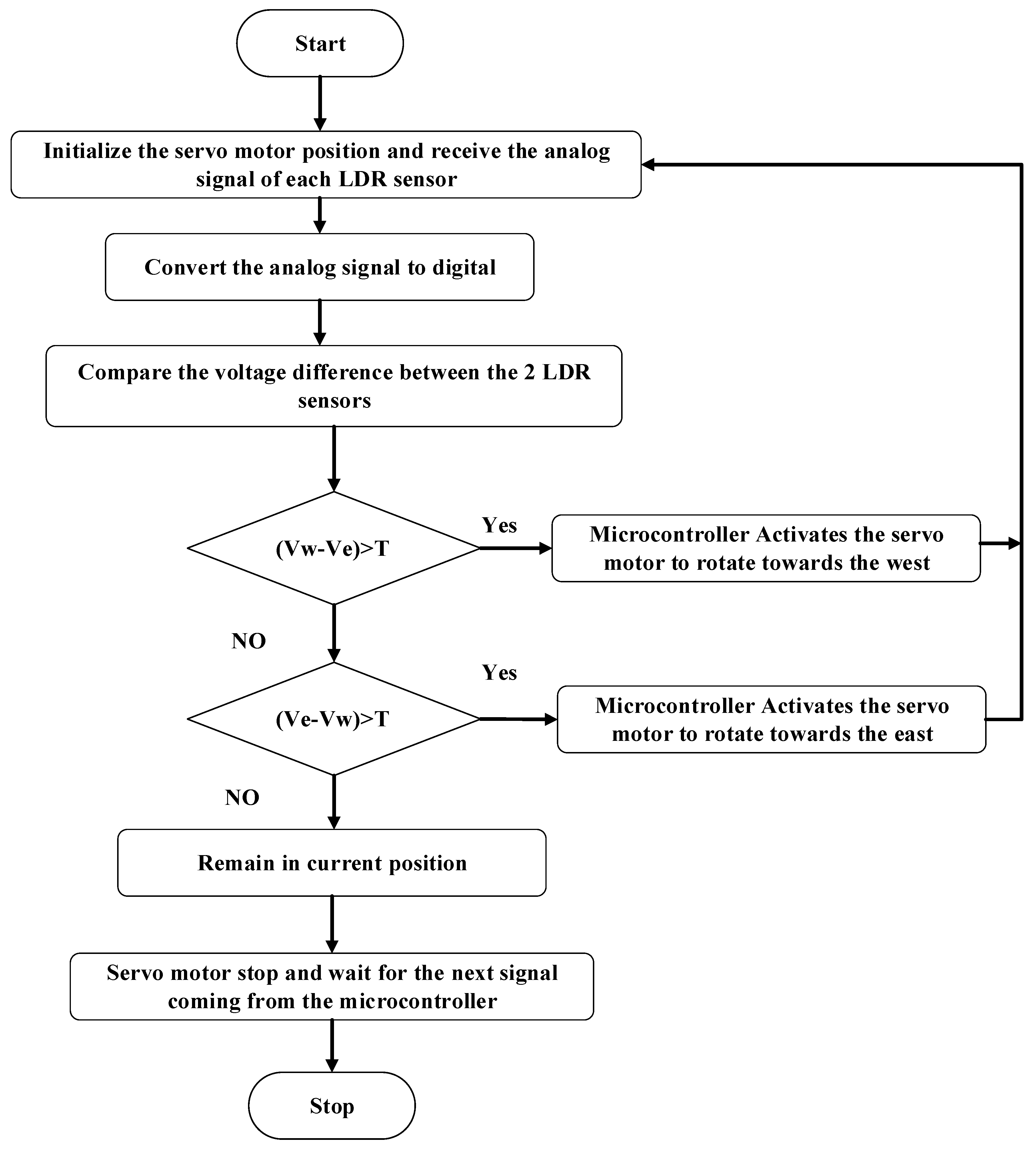
3.1.5. Working Principle of the Tracking System

The working principle of the single-axis solar tracking system depends on the signals received by the microcontroller from the two LDR sensors. As above-mentioned, the Arduino UNO had a set of digital and analog pins that were used as inputs and outputs. LDR sensors were connected to the analog pins, which represented the inputs of the tracking system as shown in Figure 4. The Arduino had a built-in Analog to Digital Converter (ADC) that was used for converting the analog signal from LDR sensors into a digital signal. The intensity of the light on both LDR sensors was compared together. If the intensity of the light on one LDR was more than the other LDR, a signal was sent from the Arduino to the servo motor to move in the direction of the LDR that had the highest light intensity. The solar panel moved in parallel with the servo motor movement in the same direction that had the maximum light intensity.
The input voltage, V i n , was applied to the LDR circuit. The analog output voltage, V o u t , varied based on the LDR resistance, R L D R , which varied according to the intensity of the sunlight. This is illustrated using the voltage divider equation represented below:
V o u t = V i n   R R e s i s t o r s R R e s i s t o r s + R L D R
where R R e s i s t o r s represents the total circuit resistance.
The analog output voltage was sent from each LDR to the Arduino. The microcontroller then automatically converted the analog output voltage (0–5 V) to digital output voltage from (0–1024 V) through the built-in ADC. After that, the microcontroller analyzed the data obtained and calculated the difference between the two sensor voltages. Considering that, V w represents the sensor voltage value of LDR located at the west direction and V e represents the sensor voltage value of LDR located toward the east. The difference between the two sensors was then compared to the selected tolerance. When the difference between the two sensors was more than the tolerance value that had been selected, the microcontroller sent a digital signal to the servo machine to rotate the solar cell in the correlated direction, as shown in Figure 5.

3.2. Battery

Solar panels are able to produce electrical energy only when there is solar radiation. Therefore, a storage system must be provided to store the excess energy to be used in times when there is no solar radiation. The battery used in this solar system was a 12-V gel battery, (gel battery is a valve-regulated lead-acid battery (VRLA) with a gel electrolyte cell technology battery), see Figure 1c. This battery had a nominal capacity of 200 Ah. The life span of the battery was eight years. The number of batteries used was eight batteries connected, respectively, thus the total voltage became 96 V.

3.3. Charge Controller

The charge controller was one of the most important parts in this system due to the random nature of solar energy and the fluctuations that occur as a result of climatic changes. Its function was to regulate the charge and discharge of batteries to protect batteries from overcharging. The charger automatically adjusted itself to the system voltage. A 60 A MPPT solar charge controller was used in the proposed system and had a LCD to display the working status of the controller (see Figure 1c). The efficiency of the MPPT solar charge controller was higher than the traditional solar charge controller as it made the solar panel work at the optimal power point, which increased the efficiency to reach 98 percent, reducing the amount of energy lost. It had the ability to automatically recognize the system voltage and could also charge all kinds of batteries.

3.4. Inverter

Most of the load in the office building were AC loads. To take advantage of the energy obtained from the solar panels, the DC electricity had to be converted to AC electricity. This process was done by the DC–AC inverter (see Figure 1c). The rated power of the inverter was preferred to be higher than the maximum AC load by 10–25%, and in turn, the specified inverter was preferred as suitable for the charge controller. The selected inverter had a 4   kW rated power.

3.5. Load Reference

The office building studied contained:
  • lights
  • a fan, an air conditioner (1.5 HP), an extractor fan
  • a computer, a printer, and a fax machine
  • a refrigerator, an electric kettle, a water cooler
  • a sound system
Table 1 shows the values of these loads. The PV system was used to supply the loads in the office, as shown in Table 1. The load power consumed was not constant and depended on the load variation and the amount of DC power from the PV system, which in turn was influenced by the amount of irradiation received as well as the ambient temperature.

4. Estimating the Energy Consumption from the Proposed Model

To estimate the energy consumption taking into account the impact of the temperature and irradiance with the AC power consumption from the reference load connected to 4   kW DC PV modules, a proposed artificial model using an artificial neural network (ANN) was presented. The ANN considered the system as a single-axis tracking system with an array tilt of 21 ° and array azimuth of 180 ° . In addition, an estimation value from the data measured of system losses around 14.08 % and inverter efficiency of 96 % with DC to AC load size ratio of 1.2 was taken into account.

4.1. Artificial Neural Network (ANN)

An ANN is an algorithm that mimics the behavior of the human brain. This algorithm is similar to the human brain in the way it works and that distinguishes it from other techniques. It relies on non-linear mathematics, which enables it to design complex and non-linear systems.
The number of neurons and layers in an ANN model depends on the complication status of the system. The ANN finds the relationship between the input and output elements of the system by using an iterative procedure called the training phase. All input and neurons have their own related weight. Weights are numbers that are determined through the training process [32,33,34,35]. Choosing the correct parameters as inputs and outputs of the ANN is very important to build an accurate and dependable model. The availability of data for choosing parameters, system information for the identification of correlation between different parameters, and the goal for the constructing model are basic factors in selecting suitable inputs and outputs. Accuracy of the selected output parameters can be tested by sensitivity analysis.
The ANN has many advantages and disadvantages in the prediction of consumed energy, and the advantages of an ANN can be described as:
  • providing the least error in the nonlinear input;
  • has the ability to provide a relationship between input and output without complex mathematical equations;
  • learns and makes decisions easily; and
  • has flexibility in modeling.
The disadvantages of an ANN can be summarized as:
  • errors may occur in the forecasting process due to over fitting;
  • training may be unstable, which leads to errors in the forecasted model;
  • many parameters need to be determined (such as weights); and
  • the inability to use information from a small sample size and low convergence.
To overcome these disadvantages, a huge number of data could be used for training the proposed ANN.
The proposed system depended on the variation of AC power over time during each studied month in order to predict the energy consumption. The non-linearity in the proposed model that required a consideration of the ANN algorithms was the non-linearity of the system and energy consumption regarding the impacts of temperature and irradiance in this prediction.
Figure 6 shows the training structure of the ANN with five inputs, one output and 60 neurons in one hidden layer [35]. The proposed system required only one hidden layer and a maximum of 60 neurons to obtain the prediction of the consumed energy during each month with high accuracy.

4.2. Transfer (Activation) Function

Transfer (activation) functions transform the activation level of a unit (neuron) into an output signal. There are various transfer functions included in the Neural Network Toolbox in the MATLAB environment [35]. Transfer function could be placed into three categories:
  • linear transfer functions;
  • log-sigmoid transfer function; and
  • tan-sigmoid transfer function.
The suitability of the case study due to the variation of the temperature and irradiance value was the log-sigmoid transfer function. Figure 7 shows the proposed transfer functions that were used for training the neural networks.
The process to find the output is determined by:
For j t h hidden neuron, the output of the first hidden layer y j is estimated from
y j = 1 / ( 1 + exp ( ( i = 1 n w j i x i b j ) ) )   j = 1 ,   2 ,   ,   N
where x i is the i t h input; b j is the base of the first hidden layer; and w j i are the weights between the i t h input neurons and the j t h first hidden neurons.
The required output from the l t h output layer is determined by:
O l = ( j = 1 N w l j y j )       l = 1 ,   2 ,   ,   H
where w l k is the weights between the j t h first hidden neurons and the l t h output neurons.

4.3. Error Criteria

The objective in training the ANN was to minimize as many errors as possible. Minimization of errors simply means improving the performance of the training and obtaining a more accurate model. Different definitions and types of errors may be considered when training the ANN. For instance, absolute error is defined as the difference between the measured (actual) output and the desired output (target). However, it is common to use the mean square error (MSE) when training the ANN. The MSE is defined according to Equation (4), as given by [35],
M S E = 1 n i = 1 n { y m i y i y m i } 2
where y m is the measured average value of energy consumed in the office building for each hour during each month, which is the input to the system as training and check data; y is the output target that represents the prediction of the consumed energy of the proposed system; i is the number of datasets; and n is the number of training patterns.
The relative error can be used to compare the proposed estimated ANN energy consumption and the measured one.
r e l a t i v e   e r r o r = y m i y i         i = 1 ,   2 ,   , n
In addition, relative error can be utilized to update the weights of the ANN to minimize the MSE. The fitness value of the training pattern is computed by:
F i t n e s s ( X i ) = m i n ( M S E )

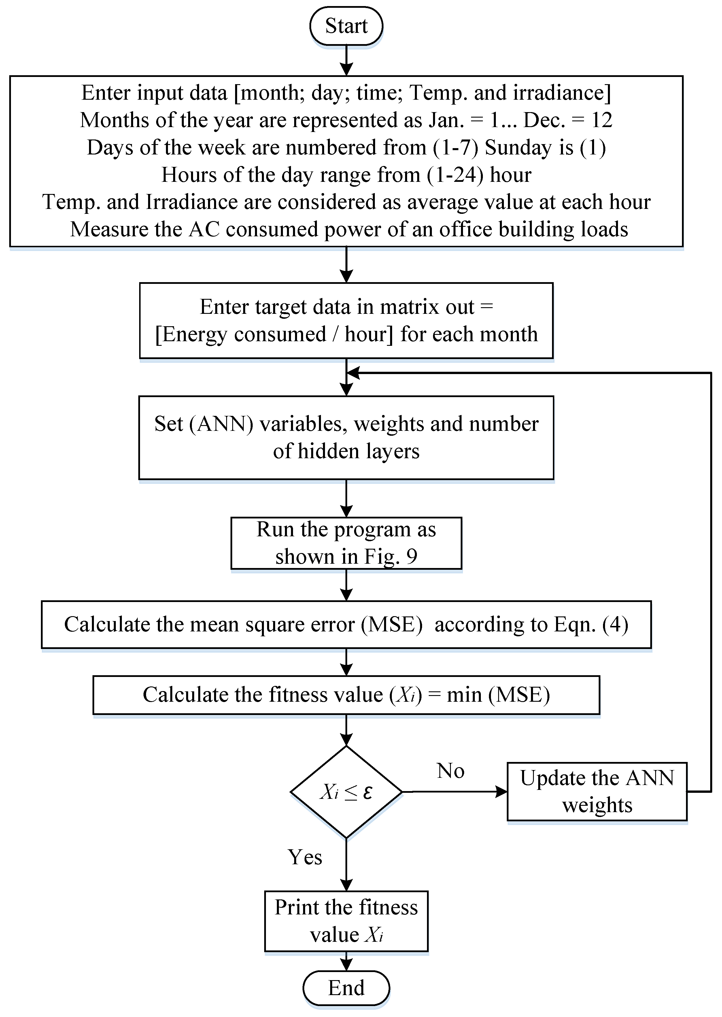
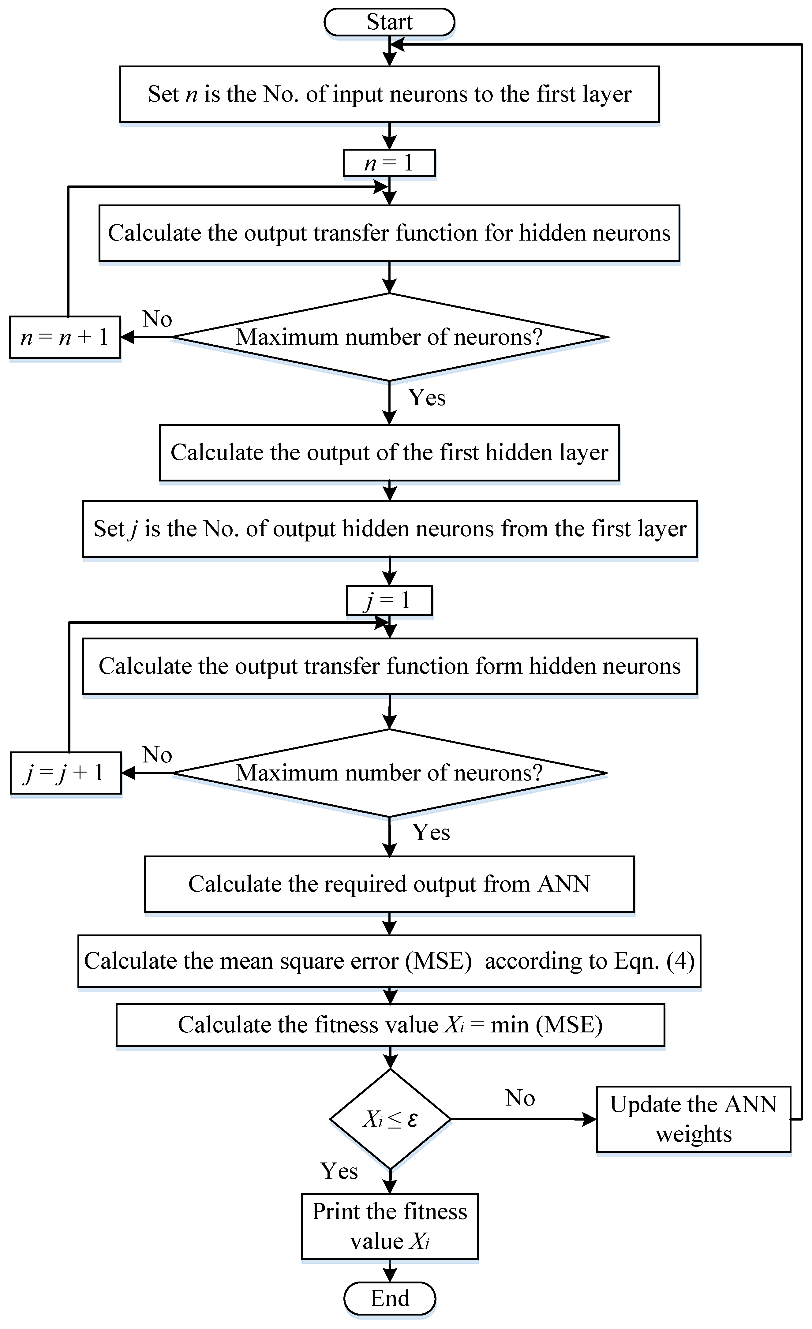
4.4. Training Methodology of the Proposed ANN

Designing an ANN model that can predict the average monthly energy consumption requires determining the number of input parameters. These parameters are:
  • the average temperature;
  • the average solar irradiance;
  • the average AC power output; and
  • months of the year and the holidays
The measured data of average solar radiation, temperature, AC consumed power of the system during each hour of the twelve months for one year considering the holidays using a wireless sensor network (for average temperature and irradiance measurement) were utilized as the input training data of the proposed ANN, as seen Figure 8.
According to the dataset of the AC load power consumption during each hour for different months, the ANN used these data for estimating the energy consumption, considering not only the AC load power, but also the average measurement values of the temperature and irradiance with time variation.
The predicted average monthly energy consumption represented the output. All variables, weights, and the number of hidden layers were adjusted. The mean square error (MSE) was calculated and compared with the target entered before, which represented the energy consumed per hour during the month system as shown in Figure 8 and Figure 9.
The training methodology of the proposed ANN in the details is clarified in Figure 9 and explains the correlation of the first hidden layer between the input neuron data and output target fitness function. The final results obtained after different updating cycle to the ANN weights depended on the MSE values until the proposed algorithm reached the minimum MSE.

5. Results Analysis

The study was conducted during the four seasons of the year in 2018 to study and analyze the seasonal performance of solar panels. A single-axis solar tracking system was used for a group of solar panels with a total capacity of 4   kW . The solar radiation, temperature, and output power of the system were measured during winter, spring, summer, and finally, autumn.

5.1. The Winter Season

The results obtained during winter were taken in December. During winter, the temperature decreases, and solar radiation is reduced. Figure 10 shows the variation of the radiation during 720 h in December. Figure 11 shows the low and largely random temperatures. The changes in temperature and irradiation affected the output power of the 4   kW solar system, as shown in Figure 12 and Figure 13.

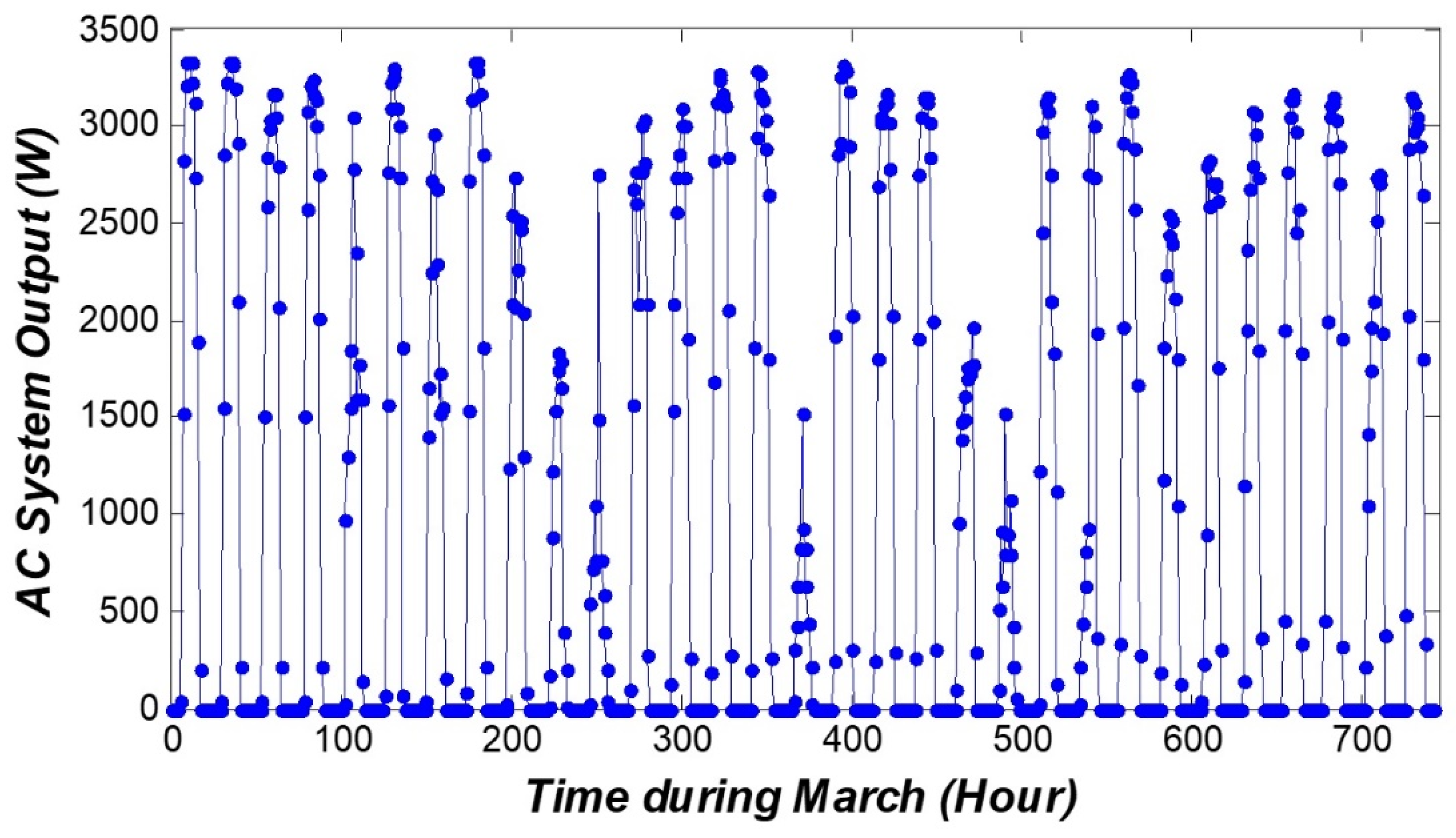
5.2. The Spring Season

The results obtained during spring were taken in March, the beginning of spring in the Northern Hemisphere. This season is characterized by its temperate climate, where the temperature and the average solar radiation are moderate as the number of daylight hours equals the number of night hours. The irradiation changes during 720 h in March are shown in Figure 14.
The temperature in spring is fairly moderate, ranging from 10 to 30 degrees during the night and day as shown in Figure 15. The changes in the output power of the solar panel during this month are shown in Figure 16 and Figure 17.

5.3. The Summer Season

The results obtained during summer were taken in June 2018. June is the beginning of summer in the Northern Hemisphere.
The summer season is the hottest season of the year and consequently, receives the most solar irradiation of all the other seasons in the year. The number of daylight hours during this season was greater than the number of hours of night. Subsequently, the solar panels underwent a longer period of exposure to solar radiation during the day.
The irradiation changes during 720 h in June are shown in Figure 18. The temperature in the summer is very high, ranging from 30 to 45 degrees during the night and day as shown in Figure 19. The changes in the output power of the solar panels during this month are shown in Figure 20 and Figure 21.

5.4. The Autumn Season

The results obtained during autumn were taken in September 2018. September is the beginning of autumn in the Northern Hemisphere. The weather in the autumn is somewhat irregular because it mediates between summer and winter. In this season, temperatures drop gradually. At the beginning of the season, the temperatures remain fairly high. As the season progresses, temperatures gradually decline to signal the transformation from autumn to winter. The irradiation changes during 720 h in September are shown in Figure 22. The temperature in autumn is very irregular, ranging from 25 to 42 degrees during the night and day as shown in Figure 23. The changes in the output power of the solar panel during this month are shown in Figure 24 and Figure 25.

5.5. Estimating the Energy Consumption Using ANN

In the proposed model of the 4 kW DC system PV modules of single-axis tracking system with an array tilt angle 21 ° and an array azimuth of 180 ° , considering system losses of 14.08 % and inverter efficiency of 96 % with DC to AC load size ratio of 1.2 , the energy consumption estimation using the ANN during one year was investigated and the results are explained in Table 2.
From Table 2, the average AC energy consumption estimated from the proposed model for the case study was around 8431   ( kWh / Year ) , which represents the efficiency of the proposed model under the impact of the temperature and solar irradiance.

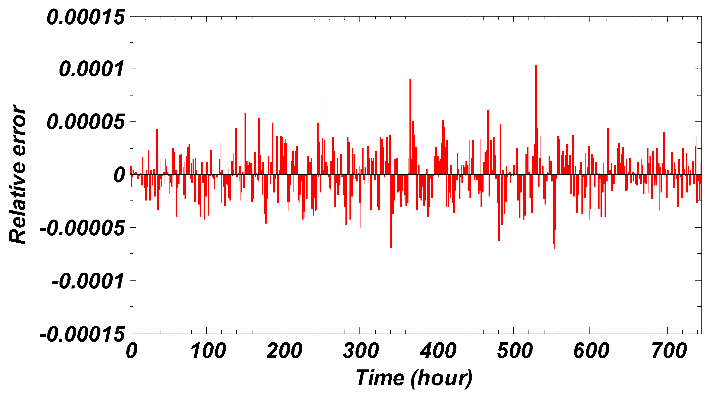
5.6. Relative Error (Accuracy of Proposed ANN)

In order to assess the accuracy of the proposed ANN, the relative error between the ANN proposed estimated value of energy consumption and the measured one was investigated.
The maximum absolute value of the relative error did not exceed 2 × 10 4 during the whole investigated year. This indicates that the proposed ANN for the estimated energy consumption provided good results with high accuracy.
Figure 26, Figure 27, Figure 28 and Figure 29 give different examples of the calculated relative error during different months that represent different seasons during the year. From these figures, it is clear that the proposed ANN estimated value increased or decreased from the measured value in a very small and limited error of around 2 × 10 4 .

6. Conclusions

Looking at the obtained results, it is evident that solar cell performance was higher at moderate temperatures. It is clear from the results that during the spring season, the efficiency of the solar panel was very high compared to the other seasons. The output power reached about 3250 W during this season, which was the highest reached out of all four seasons. This was due to the presence of high radiation of about 990 W/m2 and moderate temperature (high/low) about (33/18) degrees in spring. For radiation conditions with different temperatures during the four seasons, it was found that the solar panels did not produce the same power. The increase in solar radiation led to an increase in output power. Despite obtaining the highest power from the solar panels during spring, the output power was irregular due to the climatic changes during this season. In this season, temperatures rose and fell as well as experiencing irregular solar radiation. During autumn and summer, the resulting power was most regular due to the stability of solar radiation and temperature. Estimating energy consumption using an ANN was presented during the year considering the impacts of temperature and irradiance for the 4   kW PV modules used in an office building. The single-axis tracking system in operation with an array tilt angle of 21 ° and an array azimuth of 180 ° was taken into account as well as system losses of 14.08 % with an inverter efficiency of 96 % and DC–AC load size ratio of 1.2 . The results obtained from the ANN with 60 neurons for the value of energy consumption was given of around 8431   ( kWh / Year ) for the average solar radiation of 7.93   ( kWh / m 2 / Year ) and maximum average temperature of 33   ° C . The maximum relative error of the proposed ANN estimated energy algorithms did not exceed 2 × 10 4 .

Author Contributions

Formal analysis, M.T.; Investigation, A.A., M.H.E. and M.T.; Methodology, M.T.; Project administration, A.A.; Supervision, M.T.

Funding

This work was funded by the Deanship of Scientific Research at Shaqra University under the project grant number D180000/G01/N052.

Acknowledgments

The authors would like to take this opportunity to express profound gratitude and deep regards toward the Deanship of Scientific Research at Shaqra University for their generous grant covering this research under the project grant number D180000/G01/N052.

Conflicts of Interest

The authors confirm that there are no conflicts of interest.

References

  1. Chen, Y.; Zhao, J.; Lai, Z.; Wang, Z.; Xia, H. Exploring the effects of economic growth, and renewable and non-renewable energy consumption on China’s CO2 emissions: Evidence from a regional panel analysis. Renew. Energy 2019, 140, 341–353. [Google Scholar] [CrossRef]
  2. Amri, F. Renewable and non-renewable categories of energy consumption and trade: Do the development degree and the industrialization degree matter? Energy 2019, 173, 374–383. [Google Scholar] [CrossRef]
  3. Aly, S.P.; Ahzi, S.; Barth, N. An adaptive modelling technique for parameters extraction of photovoltaic devices under varying sunlight and temperature conditions. Appl. Energy 2019, 236, 728–742. [Google Scholar] [CrossRef]
  4. Renewables 2018: Global Status Report; REN21: Paris, France, 2018. (In English)
  5. Hafez, A.Z.; Yousef, A.M.; Harag, N.M. Solar tracking systems: Technologies and trackers drive types-A review. Energy Rev. 2018, 91, 754–782. [Google Scholar] [CrossRef]
  6. Alblawi, A.; Zainuddin, N.; Roslan, R.; Rahimi-Gorji, M.; Bakar, N.A.; Do, H. Effect of heat generation on mixed convection in porous cavity with sinusoidal heated moving lid and uniformly heated or cooled bottom walls. Microsyst Technol. 2019. [Google Scholar] [CrossRef]
  7. Fébba, D.; Rubinger, R.; Oliveira, A.; Bortoni, E. Impacts of temperature and irradiance on polycrystalline silicon solar cells parameters. Sol. Energy 2018, 174, 628–639. [Google Scholar] [CrossRef]
  8. Zhang, J.; Liu, J.; Liu, C. An algebra method to fast track the maximum power of solar cell via voltage, irradiance and temperature. Optik 2018, 174, 332–338. [Google Scholar] [CrossRef]
  9. Vasel, A.; Iakovidis, F. The effect of wind direction on the performance of solar PV plants. Energy Convers. Manag. 2017, 153, 455–461. [Google Scholar] [CrossRef]
  10. El Achouby, H.; Zaimi, M.; Ibral, A.; Assaid, E. New analytical approach for modelling effects of temperature and irradiance on physical parameters of photovoltaic solar module. Energy Convers. Manag. 2018, 177, 258–271. [Google Scholar] [CrossRef]
  11. Ibrahim, H.; Anani, N. Variations of PV module parameters with irradiance and temperature. Energy Procedia 2017, 134, 276–285. [Google Scholar] [CrossRef]
  12. Elbaset, A.A.; Ali, H.; el Sattar, M.A. New seven parameters model for amorphous silicon and thin film PV modules based on solar irradiance. Sol. Energy 2016, 138, 26–35. [Google Scholar] [CrossRef]
  13. Perrak, V.; Kounavis, I.P. Effect of temperature and radiation on the parameters of photovoltaic modules. J. Renew. Sustain. Energy 2016, 8, 013102. [Google Scholar] [CrossRef]
  14. Mandadapu, U.; Vedanayakam, V.; Thyagarajan, K. Effect of Temperature and Irradiance on the Electrical Performance of a Pv Module. Int. J. Adv. Res. 2017, 5, 2018–2027. [Google Scholar] [CrossRef]
  15. Aller, J.; Viola, J.; Quizhpi, F.; Restrepo, J.; Ginart, A.; Salazar, A. Explicit Model of PV Cells considering variations in temperature and solar irradiance. In Proceedings of the 2016 IEEE Andescon, Arequipa, Peru, 19–21 October 2016; pp. 1–4. [Google Scholar]
  16. Ruschel, C.S.; Gasparin, F.P.; Costa, E.R.; Krenzinger, A. Assessment of PV modules shunt resistance dependence on solar irradiance. Sol. Energy 2016, 133, 35–43. [Google Scholar] [CrossRef]
  17. Peng, L.; Zheng, S.; Chai, X.; Li, L. A novel tangent error maximum power point tracking algorithm for photovoltaic system under fast multi-changing solar irradiances. Appl. Energy 2018, 210, 303–316. [Google Scholar] [CrossRef]
  18. Akhsassi, M.; Fathi, A.; Aarich, N.E.; Bennouna, A.; Raoufi, M.; Outzourhit, A. Experimental investigation and modeling of the thermal behavior of a solar PV module. Sol. Energy Mater. Sol. Cells 2018, 180, 271–279. [Google Scholar] [CrossRef]
  19. Coskun, C.; Toygar, U.; Sarpdag, O.; Oktay, Z. Sensitivity analysis of implicit correlations for photovoltaic module temperature: A review. J. Clean. Prod. 2017, 164, 1474–1485. [Google Scholar] [CrossRef]
  20. Copper, J.K.; Sproul, A.B.; Jarnason, S. Photovoltaic (PV) performance modelling in the absence of onsite measured plane of array irradiance (POA) and module temperature. Renew. Energy 2016, 86, 760–769. [Google Scholar] [CrossRef]
  21. Talaat, M.; Farahat, M.A.; Elkholy, M.H. Renewable power integration: Experimental and simulation study to investigate the ability of integrating wave, solar and wind energies. Energy 2019, 170, 668–682. [Google Scholar] [CrossRef]
  22. Talaat, M.; Alsayyari, A.S.; Essa, M.A.; Yousef, M.A. Investigation of transparent pyramidal covers effect to PV power output using detected wireless sensors incident radiation. Measurement 2019, 136, 775–785. [Google Scholar] [CrossRef]
  23. Widyolar, B.; Abdelhamid, M.; Jiang, L.; Winston, R.; Yablonovitch, E.; Scranton, G.; Cygan, D.; Abbasi, H.; Kozlov, A. Design, simulation and experimental characterization of a novel parabolic trough hybrid solar photovoltaic/thermal (PV/T) collector. Renew. Energy 2017, 101, 1379–1389. [Google Scholar] [CrossRef]
  24. Akarslan, E.; Hocaoglu, F.O.; Edizkan, R. Novel short term solar irradiance forecasting models. Renew. Energy 2018, 123, 58–66. [Google Scholar] [CrossRef]
  25. Hocaoglu, F.O.; Serttas, F. A novel hybrid (Mycielski-Markov) model for hourly solar radiation forecasting. Renew. Energy 2017, 108, 635–643. [Google Scholar] [CrossRef]
  26. Akarslan, E.; Hocaoglu, F.O. A novel method based on similarity for hourly solar irradiance forecasting. Renew. Energy 2017, 112, 337–346. [Google Scholar] [CrossRef]
  27. Boilley, A.; Thomas, C.; Marchand, M.; Wey, E.; Blanc, P. The Solar Forecast Similarity Method: A New Method to Compute Solar Radiation Forecasts for the Next Day. Energy Procedia 2016, 91, 1018–1023. [Google Scholar] [CrossRef]
  28. Voyant, C.; Notton, G.; Kalogirou, S.; Nivet, M.L.; Paoli, C.; Motte, F.; Fouilloy, A. Machine learning methods for solar radiation forecasting: A review. Renew. Energy 2017, 105, 569–582. [Google Scholar] [CrossRef]
  29. Khosravi, A.; Koury, R.N.N.; Machado, L.; Pabon, J.J.G. Prediction of hourly solar radiation in Abu Musa Island using machine learning algorithms. J. Clean. Prod. 2018, 176, 63–75. [Google Scholar] [CrossRef]
  30. Fouilloy, A.; Voyant, C.; Notton, G.; Motte, F.; Paoli, C.; Nivet, M.L.; Guillot, E.; Duchaud, J.L. Solar irradiation prediction with machine learning: Forecasting models selection method depending on weather variability. Energy 2018, 165, 620–629. [Google Scholar] [CrossRef]
  31. Talaat, M.; Hatata, A.Y.; Abdulaziz; Alsayyari, S.; Alblawi, A. A smart load management system based on the grasshopper optimization algorithm using the underfrequency load shedding approach. Energy 2019, 116423. [Google Scholar] [CrossRef]
  32. Alzahrani, A.; Shamsi, P.; Dagli, C.; Ferdowsi, M. Solar Irradiance Forecasting Using Deep Neural Networks. Procedia Comput. Sci. 2017, 114, 304–313. [Google Scholar] [CrossRef]
  33. Yaïci, W.; Longo, M.; Entchev, E.; Foiadelli, F.J.S. Simulation study on the effect of reduced inputs of artificial neural networks on the predictive performance of the solar energy system. Sustainability 2017, 9, 1382. [Google Scholar] [CrossRef] [Green Version]
  34. Jassim, H.; Lu, W.; Olofsson, T.J.S. Predicting energy consumption and CO2 emissions of excavators in earthwork operations: An artificial neural network model. Sustainability 2017, 9, 1257. [Google Scholar] [CrossRef] [Green Version]
  35. Talaat, M.; Gobran, M.H.; Wasfi, M. A hybrid model of an artificial neural network with thermodynamic model for system diagnosis of electrical power plant gas turbine. Eng. Appl. Artif. Intell. 2018, 68, 222–235. [Google Scholar] [CrossRef]
Figure 1. Photovoltaic 4   kW system. (a) Photographic recording of 4   kW Photovoltaic (PV) modules, (b) single-axis solar tracker with automatic control system, (c) a schematic diagram of the PV system.
Sustainability 11 06802 g001
Figure 2. Block diagram of the single-axis solar tracker.
Sustainability 11 06802 g002
Figure 3. Variation of LDR efficiency with solar radiation.
Sustainability 11 06802 g003
Figure 4. Wiring circuit of the single-axis solar tracking system.
Sustainability 11 06802 g004
Figure 5. Single-axis solar tracking system flowchart.
Sustainability 11 06802 g005
Figure 6. Structure of the proposed model of the ANN.
Sustainability 11 06802 g006
Figure 7. Log-sigmoid transfer function.
Sustainability 11 06802 g007
Figure 8. Consumed energy estimation based on ANN training.
Sustainability 11 06802 g008
Figure 9. Training methodology of the proposed ANN.
Sustainability 11 06802 g009
Figure 10. The irradiation changes during 720 h in December.
Sustainability 11 06802 g010
Figure 11. Ambient temperature changes during 720 h in December.
Sustainability 11 06802 g011
Figure 12. DC array output power in December.
Sustainability 11 06802 g012
Figure 13. AC system output power in December.
Sustainability 11 06802 g013
Figure 14. The irradiation changes during 720 h in March.
Sustainability 11 06802 g014
Figure 15. Ambient temperature changes during 720 h in March.
Sustainability 11 06802 g015
Figure 16. DC array output power in March.
Sustainability 11 06802 g016
Figure 17. AC system output power in March.
Sustainability 11 06802 g017
Figure 18. The irradiation changes during 720 h in June.
Sustainability 11 06802 g018
Figure 19. Ambient temperature changes during 720 h in June.
Sustainability 11 06802 g019
Figure 20. DC array output power in June.
Sustainability 11 06802 g020
Figure 21. AC system output power in June.
Sustainability 11 06802 g021
Figure 22. The irradiation changes during 720 h in September.
Sustainability 11 06802 g022
Figure 23. Ambient temperature changes during 720 h in September.
Sustainability 11 06802 g023
Figure 24. DC array output power in September.
Sustainability 11 06802 g024
Figure 25. AC system output power in September.
Sustainability 11 06802 g025
Figure 26. Relative error between the estimated and measured energy consumption during December.
Sustainability 11 06802 g026
Figure 27. Relative error between the estimated and measured energy consumption during March.
Sustainability 11 06802 g027
Figure 28. Relative error between the estimated and measured energy consumption during June.
Sustainability 11 06802 g028
Figure 29. Relative error between the estimated and measured energy consumption during September.
Sustainability 11 06802 g029
Table 1. Loads of an office building in Dawadmi, Saudi Arabia.
Load TypeLoad’s (Watt)No.Total (Watt)
Lights11 W10110 W
Fan80 W2160 W
Computer150 W2300 W
Printer250 W1250 W
Fax machine150 W1150 W
Electric kettle1200 W11200 W
water cooler550 W1550 W
Air conditioner (1.5 HP)1120 W11120 W
Extractor Fan12 W224 W
Sound System84 W184 W
Total 3948 W
Table 2. Energy consumption estimation resulting from the ANN during one year for a 4   kW PV system used to supply the load of an office building in Dawadmi, Saudi Arabia.
MonthAverage Solar Radiation
( k W h / m 2 / d a y )
Average High Temperature (°C)AC Energy ( k W h )
January6.7821662
February7.3723633
March7.6627722
April7.7733688
May8.5139749
June9.1442771
July8.9243778
August8.9243765
September8.9640746
October8.6535767
November6.9328607
December5.5922543
Annual 7.93   ( kWh / m 2 / Year ) 33 °C 8431   ( kWh / Year )

