Article

Delineation of Urban Growth Boundaries Using a Patch-Based Cellular Automata Model under Multiple Spatial and Socio-Economic Scenarios

1
Department of Land Resource Management, School of Public Administration, China University of Geosciences, Wuhan 430074, China
2
Key Labs of Law Evaluation of Ministry of Land and Resources of China, School of Public Administration, China University of Geosciences, Wuhan 430074, China
3
Center for Applied Geographic Information Science, the University of North Carolina at Charlotte, Charlotte, NC 28223, USA
4
Department of Geography and Earth Sciences, the University of North Carolina at Charlotte, Charlotte, NC 28223, USA
*
Author to whom correspondence should be addressed.
Sustainability 2019, 11(21), 6159; https://doi.org/10.3390/su11216159
Submission received: 30 September 2019 / Accepted: 22 October 2019 / Published: 4 November 2019

Abstract

:
The urban growth boundary (UGB) plays an important role in the regulation of urban sprawl and the conservation of natural ecosystems. The delineation of UGBs is a common strategy in urban planning, especially in metropolitan areas undergoing fast expansion. However, reliable tools for the delineation of informed UGBs are still not widely available for planners. In this study, a patch-based cellular automaton (CA) model was applied to build UGBs, in which urban expansions were represented as organic and spontaneous patch growing processes. The proposed CA model enables the modeler to build various spatial and socio-economic scenarios for UGB delineation. Parameters that control the patch size and shape, along with the spatial compactness of an urban growth pattern, were optimized using a genetic algorithm. A random forest model was employed to estimate the probability of urban development. Six scenarios in terms of the demand and the spatial pattern of urban land allocation were constructed to generate UGB alternatives based on the simulated urban land maps from the CA model. Application of the proposed model in Ezhou, China from 2004 to 2030 reveals that the model proposed in this study can help urban planners make informed decisions on the delineation of UGBs under different scenarios.

1. Introduction

Future urban sprawl is estimated to cause a more than 3.7% decrease of global grain production by 2030, which will significantly aggravate food shortages in many developing countries [1]. Moreover, the intactness of biodiversity, in many biomes, has been pushed beyond the safe boundary due to uncontrolled urban growth [2]. Therefore, several strategies, such as green belts, urban service boundaries (USBs), and urban growth boundaries (UGBs), are applied worldwide to effectively regulate urban growth into a sustainable pathway [3], among which the UGB is attested to be the most successful one. A UGB is a demarcation line that distinguishes regions for urban development and areas for natural conservation and agricultural production [4]. Both practitioners and researchers have confirmed the effectiveness of UGBs in suppressing unplanned urban expansion, in promoting the efficiency of urban infrastructures, and in conserving natural ecosystems [4,5]. Many cities in the United States (such as Maryland, Florida, Minnesota, and Oregon) established UGB in the 20th century to direct sustainable urban growth [6]. Cities in other countries, such as Australia [7], Korea [8], Canada [9], and India [10], also adopted UGB. Notably, the Chinese government recently adapted its traditional strategies (which often failed in forbidding the uncontrolled urban expansion) of urban development management to a universal policy of delineating UGBs in more than 3000 cities and towns [11]. However, many of these UGBs were established based on empirical knowledge without quantitative and scientific support [3], due to the lack of appropriate tools. This deficiency highlights the necessities of appropriate and feasible means to delineate UGBs under different scenarios of urban development.
Approaches regarding the delineation of UGB generally fall into two groups. The first group directly simulates the radial expansion of UGB along different azimuths. Radial growth for UGBs is estimated based on the relationships between the driving factors and the distance from the city centers to the intersection points in the existing UGBs with the straight lines in different directions. The spatial relationship is usually estimated utilizing spatial logistic regression or artificial neural networks [12,13,14]. These radial-based UGB models were first put forward by Tayyebi, Pijanowski, and Pekin [13], and were later advanced by integrating natural obstacles and more driving factors and temporal periods to increase reliability and reduce uncertainty [11]. The major limitation of these radial-based UGB models is that they cannot reveal the spatial details of urban growth (for example, the spatial pattern and interactions between urban parcels). Moreover, it is inconvenient to conduct what-if analysis using these models. Additionally, these models do not sufficiently consider the constraints of wild space conservation on UGB delineation.
The other group of approaches delineate UGBs by identifying the outlines of the mosaics of future urban landscapes, which are usually simulated utilizing land change models, such as cellular automata (CA) and agent-based models (ABMs). The advantage of ABMs lies in its ability to represent the behaviors of decisionmakers (such as landowners and developers) and their interactions with each other and with the environment [15]. However, development, calibration, and validation of the structure, process, and output of ABMs for urban simulation require large volumes of spatial-temporal individual data, which are often challenging to collect [16]. These limitations have imposed a knowing–doing gap for urban planners looking to use ABMs in their practice of UGB delineation. Comparatively, CA is a more popular simulation tool that is easier to implement, because of its flexibility in model structure and seamless integration with Geographic Information Systems [17]. Many researchers have used the CA model since the 1990s to support urban planning design, to explain the mechanisms of urban sprawl, and to identify the potentially adverse effects raised from urban expansion. Additionally, several CA-based UGB models have been developed in combination with other techniques in recent years [18,19,20].
However, conventional CA models for UGB delineation usually utilize a cell-based simulation engine in which urban expansion is expressed as the state transition of individual pixels, while, in reality, urban developments are typically implemented in parcels. To alleviate this biased representation of the urban development procedure, an alternative form of CA model, which is patch-based CA, is used. In a patch-based CA, urban land parcels are represented by irregular raster patches. A raster patch is a collection of regular lattices that have the same state and are spatially connected. Researches have validated the superiority of patch-based CA models over cell-based ones in the simulation of urban growth [21,22,23,24,25], as well as the UGB delineation [26].
A major limitation in the delineation of UGBs using patch-based CA models lies in the disability of allowing the scenario builders to carefully control the spatial pattern of the future urban landscape, which is of importance for urban planners to understand the potential impacts of their spatial preferences on the resulting UGBs. For instance, some urban planners may want to conduct what-if analysis by simultaneously tuning the patch size, shape, and the spatial compactness of urban patch allocation when demarcating UGBs. Although several studies have tried to generate UGB under a single scenario [11,12,13,20], scenarios that simultaneously consider the urban development demand and spatial pattern of urban growth allocation have not yet been adequately explored for UGB generation.
Therefore, the purpose of this study was to build a patch-based CA model that allows for the establishment of spatial scenarios for the delineation of UGBs. The CA model uses two parameterized and self-organized patch growing functions to represent two different spatial progress of urban development: organic urban growth, which dedicates the expansion of existing urban patches, and spontaneous urban growth, which depicts the initialization and self-growing of isolated urban patches. These two spatial progressions of urban development occur and agglomerate to generate various urban landscapes. Parameters were designed in the proposed CA model for urban planners to control the patch size, shape, and compactness of urban growth when delineating UGBs. In this study, we focused on the following two research questions: first, we attempted to assess the reliability and feasibility of the proposed patch-based CA model in a simulation of realistic urban growth; second, we showcased how spatial compactness of patch layout impacts the outputs of scenario-based delineation of UGBs. The application of the UGB delineation framework was conducted in a rapidly growing city in central China, where various policies have been implemented to direct sustainable urban growth and to protect farmlands and open spaces.

2. Study Area and Data

2.1. Study Area

The study area is a satellite city of the capital of Hubei province, China (see Figure 1). The total area of this region is 1593 km2 and was inhabited by around 1.3 million people in 2016, with more than half living in the urban areas. The study area has various ecosystems and natural habitats for biodiversity conservation. Notably, the wetland system in Ezhou is essential in the local freshwater provision and the preservation of migratory birds. Additionally, Ezhou is a major grain-producing region in central China and a national pilot city of urban-rural integration development. Therefore, many land use policies are initially implemented and evaluated here before they are applied across the country. These policies have vastly provoked the economic and population explosion in this region. Consequently, rapid urban expansion has been observed in recent years (see Figure 2) and has exerted considerable pressure on the sustainable grain production and conservation of natural habitats for wildlife, especially palmipeds [27,28]. Therefore, the local government has launched a series of land use policies [29,30] to shape urban growth by conserving largely-undeveloped wildland around towns, such as the permanent farmland zone, the ecological red line strategy [31], and the urban–rural linked construction policy [32]. Among these policies, the UGB delineation strategy plays an indispensable role in guiding urban growth to a more sustainable pathway. However, the current UGBs in the study area were mainly drawn empirically by urban planners. Thus, sophisticated tools that support informed delineation of UGBs are in urgent need.

2.2. Data

Vector-based land use and land cover maps in 2004, 2009, and 2016 were obtained from the local government to calibrate and validate the patch-based CA model. These LULC maps were produced using a human–computer interaction method based on the Landsat and SPOT satellite images. Essential pre-processing steps, such as radiometric and geometric correction, orthorectification, projection, and coordinate transformation were applied by the local Department of Land Surveying to eliminate or reduce the errors in these images before interpretation. Then, the department officers classified different land use/cover types using visual interpretation and field investigation methods. The overall accuracy of the interpreted LULC maps is over 90% [33]. The original LULC maps consist of multiple thematic land use/cover types, including (i) irrigated and rainfed farmland; (ii) forest and grassland with different canopy densities; (iii) wetlands, such as rivers, lakes, and shoals; (iv) rural construction land; (v) urban land, such as residential, industrial, commercial, and transport land; and (vi) other lands, such as bare, mines, and other open space. In this study, the urban-related LULC categories were aggregated as the urban land type, and all the other LULC categories were dissolved as non-urban types. Figure 2 presents the land use/cover maps.
A bevy of factors was prepared to evaluate the probability of urban development in the study area. These factors included elevation, slope, soil quality, kernel density of points-of-interest (POI), and other distance-based variables. The digital elevation model (DEM) data with a 30 m × 30 m spatial resolution was from NASA Shuttle Radar Topography Mission (SRTM) data and was provided by the Geospatial Data Cloud (http://www.gscloud.cn). The slope was derived from the DEM data. The local department of soil surveying provided the soil quality data. The POI data was retrieved from the Baidu web map [34], which shows the spatial distribution of various public infrastructures, such as shopping malls, restaurants, and schools in 2010. The spatial clustering pattern of these POIs was estimated using the kernel density function in which the bandwidth was determined following Silverman′s rule of thumb [35]. The cost-based distance of each cell to the selected spatial entities (i.e., city center, town center, railway station, highway entrance, and major water body) was calculated to represent the attractiveness of these locations. The transportation layers that show the major road, local road, highways, and railways were obtained from the Department of Transportation in the study area (http://www.ezgl.cn/). All variables were prepared and processed in ESRI ArcMap 10.4.1 [36] and rescaled to the interval (0, 1) for estimation of urban development probability. All the spatial data were resampled to a 60 m × 60 m spatial resolution given the substantial computation burden during the auto-calibration of model parameters using an optimization algorithm (see Section 3.5). Besides, the urban population data from 1978 to 2016 in the study area were collected from the Bureau of Statistics to estimate the future demand of urban development.
A important role of UGBs is to preserve ecologically-important areas that provide valuable eco-services for human beings. Thus, regions that play an indispensable role in eco-services’ provision should be identified and preserved before delineating UGBs. In this study, these ecologically protected areas were directly derived from the land use plan that was released by the local government. The land use planners identified these protected areas using a multi-criteria evaluation and analytical hierarchy process, based on factors such as vegetation type, soil property, land use, topography, and soil erosion [37]. The protected areas identified involve natural reserves, public parks, wetlands, natural forests with dense canopies, a source area of drinking water, and regions that are undergoing or very likely to suffer from severe soil erosion due to the rapid urbanization process in the study area (as presented in Figure 3). These areas were treated as constraints of future urban growth, and thus, were filtered out from the UGBs.

3. Methodology

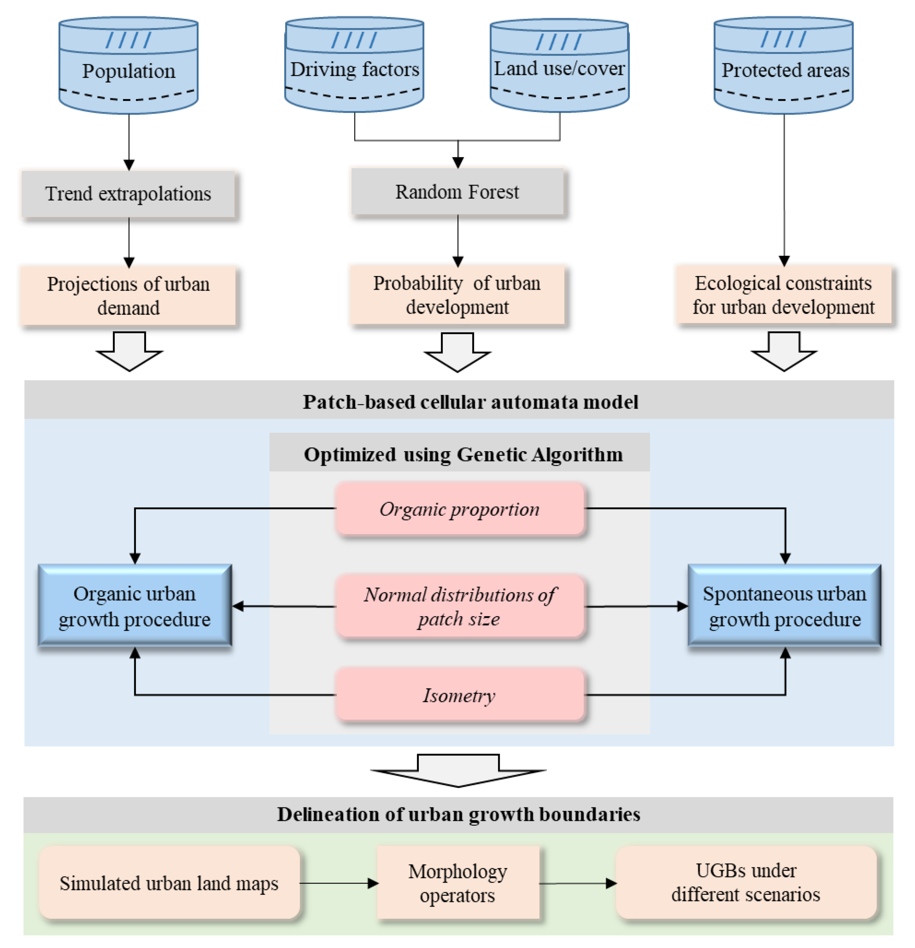
3.1. General Procedure

The UGB delineation framework proposed in this study involves several modules, as shown in Figure 4. First, the total urban land demands were projected based on linear extrapolations of historical observations in different time intervals and the per-capita urban land requirement (Section 3.2). Second, a patch-based CA model was constructed to simulate urban growth (Section 3.4), in which the urban development probability was estimated using a random forest algorithm (Section 3.3), and the key model parameters were optimized utilizing a genetic algorithm (Section 3.5). The proposed CA model represents urban growth using two processes: organic and spontaneous urban growth. During the simulation process, a specific percentage of the urban demand was allocated through the organic growth process, and the spontaneous growth process spatialized the remaining urban land. Third, urban growth under multiple spatial and socio-economic scenarios (Section 3.7) was simulated using the patch-based CA model. Finally, urban land maps from multiple model runs were aggregated, morphologically modified, and vectorized to generate UGB alternatives.

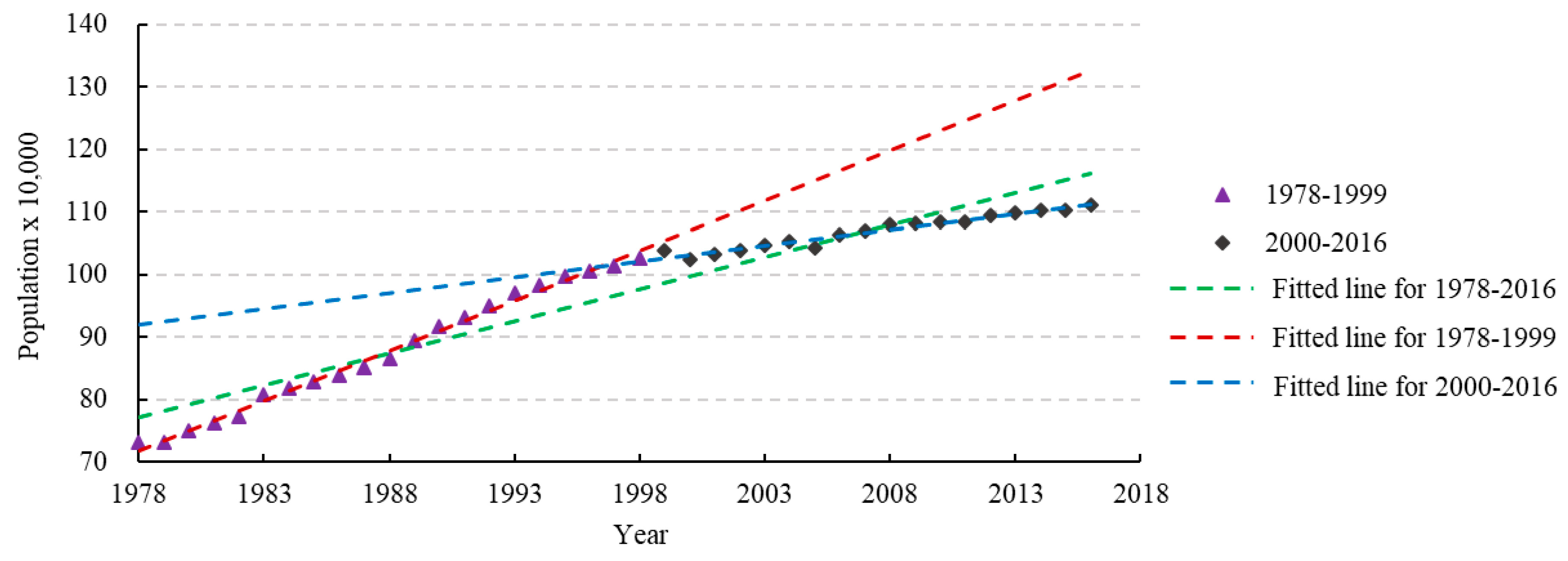
3.2. Projection of Urban Development Demand

In this study, we applied a simple approach to estimate the demand for future urban development. This approach bases its calculation of urban demand on the projection of future population and the estimation of per capita requirements of urban land [25], as described below:
D t = P t   × d t .
where D t is the required urban land at year t. P t represents the projected population at year t. d t depicts the per capita urban land at year t.

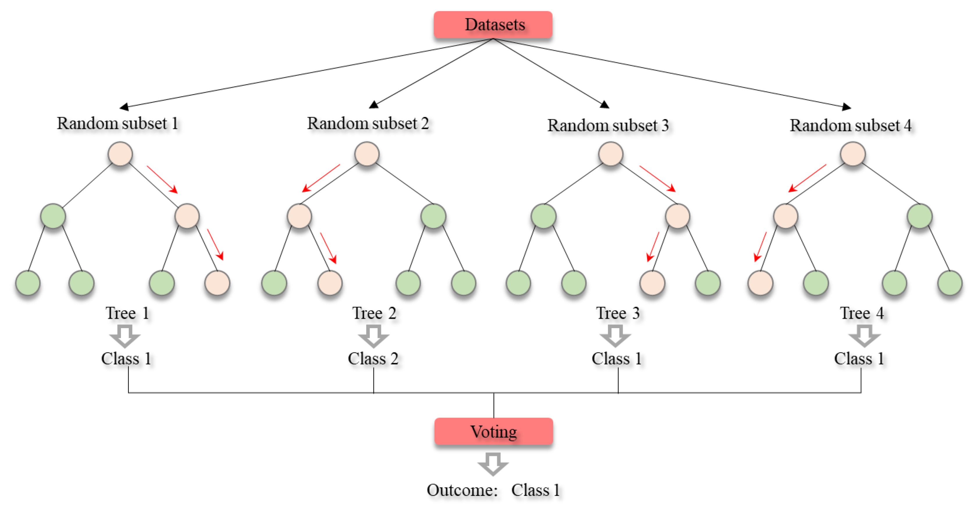
3.3. The Estimation of Urban Development Probability Using a Random Forest Algorithm

RF is a reliable, non-parametric ensemble model that ranks on the top of the classifier hierarchy. It uses the “bootstrap“ sampling strategy to create a “forest” that consists of many individual decision trees [38]. Each tree makes independent decisions based on a subset of the feature variables (i.e., determinant factors) and a random selection of the observations (i.e., training data). The final outputs of the RF model are generated by averaging the decisions of the individual trees or through a voting strategy, as shown in Figure 5. Due to the sampling strategy utilized to select the subset of variables and observations, the individual trees are constructed independently, which gives RF the merit of being insensitive to outliers, noise, and overfitting [39]. Readers are referred to Breiman [40] for more details about the RF model.
In this study, we randomly drew 12,000 points from the binary urban land change maps between 2004 and 2009 in the study area as the observations using a stratified sampling strategy. This binary variable, in which value 0 denotes “urban persistence” and value 1 depicts “non-urban to urban changes,” serves as the dependent variable in the RF model, and the independent variables were derived from the same locations in the driving factor maps. These randomly-sampled observations were used to train the RF model, which was implemented using the “Scikit-learn” package in Python 3.6 [41]. The two primary hyperparameters in the RF model, whifh are the number of features for splitting and the number of trees in the “forest,” were calibrated through a trial-and-error process in this study [42]. Finally, the number of variables for tree splitting was 5 (half of the candidate variables), and the size of the forest was 100. Then, we used the calibrated RF model to estimate the urban development probabilities for the periods of 2004–2009 and 2009–2016, respectively. The performance of the RF model was evaluated using the relative operating characteristic (ROC) curve, from which the area under the curve (AUC) was calculated to indicate the model accuracy. A value of 0.5 for the AUC value means equal performance with a random model, and a larger value indicates higher model accuracy [43].

3.4. Simulating Urban Growth Using a Patch-Based CA Model

Urban growth can be categorized into three basic types of spatial pattern; i.e., infilling, edge-expansion, and outlying (as described by Liu, et al. [44]). These three patterns were simulated using two complementary procedures in the proposed CA model: organic and spontaneous growth [23]. The organic growth process (including the infill and edge-expansion pattern) is dedicated to developing new urban patches by spreading from the inner or outer edges of an existing urban patch. Meanwhile, the spontaneous growth process (i.e., the outlying pattern) was designed to generate new urban patches that are isolated from the old ones. Both patch growing functions generate new patches following two consecutive steps: seeding and self-growing [45,46].
The seeding procedure first ranks all cells in order of their development probabilities and then keeps only a subset of cells with the highest probabilities. The expected quantity of urban development defines the number of cells that will be retained during this patch seeding process. The preserved cells then serve as candidates where new patches initialize growth. Following the pruning operation was a testing procedure to select the patch seed. To be specific, this testing operation randomly selects a cell from the pool of the candidates. If the development probability of this cell is larger than a random number that was generated from a uniform distribution in the interval of [0, 1], the cell is accepted as a seed to start a new patch. Otherwise, this testing process iterates until one seed survives. Notably, only cells that are spatially connected to existing urban patches can serve as candidates during the organic patch-growing process, and they are excluded from the alternative seeds for the spontaneous growing process. The patch self-growing procedure starts after the seeding process by centrally placing a scanning window (3 × 3 cells) on the selected seed. All neighboring cells that are available for development within this window are put into a pool, members of which serve as candidates for the self-growing of new patches. Then, another cell in this pool is selected using the same survival-testing operation. This cell is added to form the new patch if it survives the test, and the scanning window will center on this cell to add its feasible neighbors to the patch-growing pool, as shown in Figure 6. Moreover, if neighboring cells that are newly collected by this scanning window are already in the pool, their urban development probabilities are scaled down or up by multiplying a parameter termed as isometry. Then, another cell is picked and added if it survives from the test, and its neighbors are collected. The patch’s self-growing procedure continues until the expected number of cells for this new patch is reached. The isometry parameter varies from 0 to 2. Increasing this parameter will lead to a more compact patch. Specifically, the isometry parameter with a value smaller than 1 will elongate the patch, and a value larger than 1 will increase the roundness of the new patch. The sizes of a new patch are assumed to follow a normal distribution defined by the mean and variance of patch size. Another parameter designed in the patch-based CA model is the area-proportion of new patches that are generated by the organic urban growth procedure (hereafter termed as organic proportion). The organic proportion parameter impacts the spatial compactness of the simulated urban landscape. The patch growing engine keeps running until the specified urban land demand is satisfied. The organic proportion parameter, the isometry parameter, the mean, and the variance of patch size for the organic and spontaneous growing procedures can be tuned through a trial-and-error process or using heuristic optimizing approaches. In this study, we leveraged a genetic algorithm to automatically calibrate those parameters.

3.5. Calibration of the CA Parameters Using a Genetic Algorithm

The genetic algorithm (GA) is a machine learning algorithm that was inspired by the mechanism of natural evolution, and which is well suited to global optimization [48]. In the GA tool, the parameters to be optimized are encoded into an individual chromosome in a population which evolves based on the use of three stochastic operators: selection, crossover, and mutation [49,50,51]. The individual chromosome is comprised of several genes corresponding to the set of model parameters to be optimized [52]. The GA first randomly generates a number of individual chromosomes that constitute the initial population [53]. Then, the three stochastic operators are used to create new populations with the purpose of minimizing or maximizing the fitness function. The crossover operator combines two parent chromosomes to generate new individuals. The parents are selected based on a fitness maximization criterion, and individuals with fitness scores lower than a predefined threshold are removed from the population. The mutation operator moderately perturbs a chromosome by randomly changing some of the genes to avoid homogeneity among chromosomes in the population [54]. The parent chromosomes are selected using the one-to-one deterministic tournament procedure [55]. Through this heuristic searching process, a new population is assumed to inherit individuals with higher fitness from the previous generations; thus, having a larger potential to find optimal solutions for a problem [56]. The core mechanism of the GA tool used in this study was adapted from the evolving objects (EO) computation library [57]. The individuals in a new generation in the proposed GA tool generally consist of three parts: the crossover operation creates 70% of the new individuals, the mutation operation generates 1% using parent chromosomes that do not take part in the crossover procedure, and the remaining 29% are directly inherited from the original chromosomes in the previous generation [58]. Our GA kept evolving the populations until the differences among the best fitness scores in several consecutive generations were less than 5%. The individual chromosome with the highest fitness score determined the final model parameters to be applied in the subsequent validation and simulation process.
Additionally, a surrogate modeling approach [59] is applied in the GA tool to reduce the number of fitness/function evaluations during model implementation, decreasing the computational cost [60]. The surrogate approach uses a k-nearest neighbors (KNN) classifier [61] to approximate the fitness scores of some individual chromosomes based on their distance to the remaining chromosomes whose fitness scores are exactly evaluated by executing the fitness function. In this study, the fitness score of an unknown individual is assigned with the value of its nearest known individual [62]. For each generation, the fitness function of 70% of the individual chromosomes in a generation are precisely calculated, and the fitness scores of the remaining chromosomes are approximated using the surrogate model. For this remaining group, the fitness function of 70% of the individuals that have the highest fitness scores are executed by the GA tool to get their actual fitness values. These individual chromosomes are then subsequently used to update the next generation.
Moreover, to reduce the risk of overfitting in the GA tool, the variation range of each gene/parameter is limited in an envelope around the initial value of that parameter during the reproduction of new generations [58]. In this context, the initial value of model parameters is important to improve model performance. These initial values can be defined based on empirical knowledge or historical observations. More details about the GA tool are referred to in Soares-Filho, Rodrigues, and Follador [58].
We used the landscape expansion index proposed by Liu, Li, Chen, Tan, Li, and Ai [44] to evaluate the initial values for the mean and variance of patch size for the organic and spontaneous patch growth processes, and the initial value for the organic proportion parameter. The landscape expansion index categorized the new urban patches that emerged during the urban development periods of 2004–2009, 2009–2016, and 2004–2016 as infilling, edge-expansion, and outlying patterns, which could be further grouped into the two patch growing processes. For technical details about the landscape expansion index, please refer to [44]. Afterwards, we defined the initial value of the mean patch size for the two patch growing processes by correspondingly averaging the minimum and maximum values of the mean sizes of the patches for the two urban growth processes in those periods. The initial values for the variance of patch size and the organic proportion parameter were determined in the same way. The value ranges for these parameters were defined by the corresponding minimum and maximum values observed, except that the scope of the organic proportion parameter was limited to within [0, 1]. The initial values of the isometry parameter for both patch growth processes were assigned the value 1, which means no preference on patch shapes were considered, and their range was in [0, 2], as mentioned above.
The fitness function in the GA tool is represented by an index that measures the similarity between the simulated urban landscape from the CA model and the observed one. Researchers have shown that the similarity between different urban land patterns should be estimated from a neighborhood-based perspective instead of through a cell-to-cell comparison manner [63]. So far, many neighborhood-based approaches have been developed to measure pattern similarities between urban maps [64,65,66]. In this study, we adopted the reciprocal similarity comparison index proposed by AlexHagen [67] and Almeida, et al. [68] to evaluate the spatial agreement between two urban landscape patterns. This index was also used to indicate the performance of the patch-based CA model during the validation period. Notably, the index considers only the simulated changes when measuring pattern similarity; thus, avoiding biased estimation of similarity caused by the large quantity of persistence in the simulated urban maps. The size of the neighborhood window is 5 × 5 cells. Moreover, an exponential, distance-decayed function is applied to differentiate the influence of neighbors on the similarity.

3.6. Validation of the CA Model

The model parameters calibrated during the period of 2004–2009 by the GA tool may have been overfitted for the projection of future urban changes, and thus, we went through further validation. The validation process was conducted by comparing the simulated urban changes with the observed changes in a different period, 2009–2016. We used the observed area of urban development as the expected urban demand during the validation period, and the urban development probability was re-estimated with training data from urban changes in this period as well. Then, we ran the CA model multiple times with the calibrated parameters from the GA tool, and the reciprocal similarity comparison indices of the resulting urban land maps were calculated to prove the validity of the CA model.

3.7. UGB Delineation under Different Spatial Scenarios

3.7.1. Scenario Building

In this study, we built six scenarios based on demand and allocation of urban development in terms of future population growth and the spatial compactness of urban land layout. First, three projections were made for future population based on the analysis of historical demography data (see Figure 7). Then, two situations in terms of the spatial compactness of urban land allocation were introduced by varying the organic proportion parameter in the CA model. The combination of the three population projections and the two situations of urban compactness generated six scenarios.
Figure 7 shows the population growth from 1978 to 2016, which can be divided into two intervals: the fast-growing period from 1978 to 1999 and the slowly-increasing period from 2000 to 2016. Accordingly, three population growth projections were designed for future urban demand calculations. (1) Slow urban growth: Many researchers have reported that China has entered an era of low population growth, which will lead to various socio-economic problems [69]. Therefore, this scenario was designed to inspect future urban growth if the study area were to continue its low population growth tendency. In this context, the future population was linearly extrapolated from the historical populating growth trajectory between 2000 and 2016. (2) Moderate urban growth: In 2015, the Chinese government changed its childbearing policy from one-child policy [70] to a universal two-child policy [71], which should to increase the population growth rate. However, the effectiveness of this policy remains to be examined [72]. In this scenario, we assumed that the two-child policy would moderately promote future population growth. Therefore, we projected the future population in this scenario through linear extrapolation based on the population-changing trajectory between 1978 and 2016. (3) Fast urban growth: This scenario assumed that the universal two-child policy would significantly promote the future population growth rate, and thus, enlarges the demand for future urban development. To that end, we extrapolated the future population according to the historical population growth from 1978 to 1999.
The two spatial situations of urban development compactness—compact and spontaneous, are described as follows. (1) Compact urban growth: The CA model prefers the urban expansion pattern of infilling and edge-expansion, which reflects the principle of compact development in smart growth. This scenario can be realized by increasing the percentage of urban expansion that would be allocated through the organic urban growth process, which meant that the organic proportion parameter in the CA model was assigned a larger value. (2) Spontaneous urban growth: The CA model prefers the pattern of outlying urban expansion, which tends to generate a more dispersed urban pattern. This scenario was realized by increasing the percentage of urban expansion that would be allocated through the spontaneous urban growth process; thus, the organic proportion parameter in the CA model was assigned a smaller value.
Finally, six urban growth scenarios were defined as follows. Scenario 1: slow urban growth with a compact spatial pattern; Scenario 2: slow urban growth with a dispersed spatial pattern; Scenario 3: moderate urban growth with a compact spatial pattern; Scenario 4: moderate urban growth with a dispersed spatial pattern; Scenario 5: fast urban growth with a compact spatial pattern; Scenario 6: fast urban growth with a dispersed spatial pattern.

3.7.2. UGB Delineation Using Morphological Functions

We delineated UGBs based on the projections of future urban landscapes under the six scenarios. In each scenario, the CA model ran multiple replications using the calibrated model parameters (except for the organic proportion parameter), and the output urban land maps were stacked to generate an aggregated urbanization map in which the development frequency of each cell was recorded [73]. Then, the aggregated urban map was pruned according to the development frequency of cells to generate the final urban land map for UGB delineation. Specifically, we ranked the cells in the aggregated map in descending order of their simulated urbanization frequency and cut off cells in cases where the cumulative number of developed cells equaled the expected quantity of urban demand under each scenario. Afterward, two image morphology operators termed opening and closing (as detailed by Narayanan [74]) were applied to the pruned urban maps to bridge narrow gaps between urban patches and eliminate small and dispersed urban blocks [18]. The window size of the morphological operators was 3 × 3 in this study. The resulting urban land maps generated by the image morphology operators were converted to vector polygons in the ERSI ArcGIS 10.4.1 software. These polygons were then merged and dissolved to generate the UGBs, and polygons with areas smaller than 0.1 km2 were eliminated. The UGBs delineated by this process may consist of multiple parts, which is common in many Chinese cities, as reported by other researchers [75].

4. Implementation and Results

4.1. Projection of Urban Demand under Different Scenarios

The fitted extrapolation functions and the projected populations in 2030 are shown in Table 1. It can be seen that the extrapolation functions fit well with the historical trends of population growth. The goodness-of-fit (R2) values for these functions are all above 0.90. The projected population in the fast growth scenario is 1,541,260.66, which is 235,042.74 and 353,155.25 larger than those of the moderate and low population growth scenarios. Table 2 shows the projected urban land demand in 2030 if we respectively refer to the historical observations in 2004, 2009, and 2016 as the per-capita urban land requirement in 2030. We can see from Table 2 that the urban land demands in 2030 are even smaller than the actual urban area in 2016 (154.94 km2) if we take the per-capita urban land requirement in 2004 or 2009 as the reference. Comparatively, the projected urban land demand is more reasonable when the observed per capita urban requirement in 2016 was the reference. Therefore, in this study, we set the urban land demand in 2030 under the low, moderate, and the fast population growth scenarios as 165.56, 182.02, or 214.77 km2, respectively.

4.2. Calibration and Validation of the Patch-Based CA Model

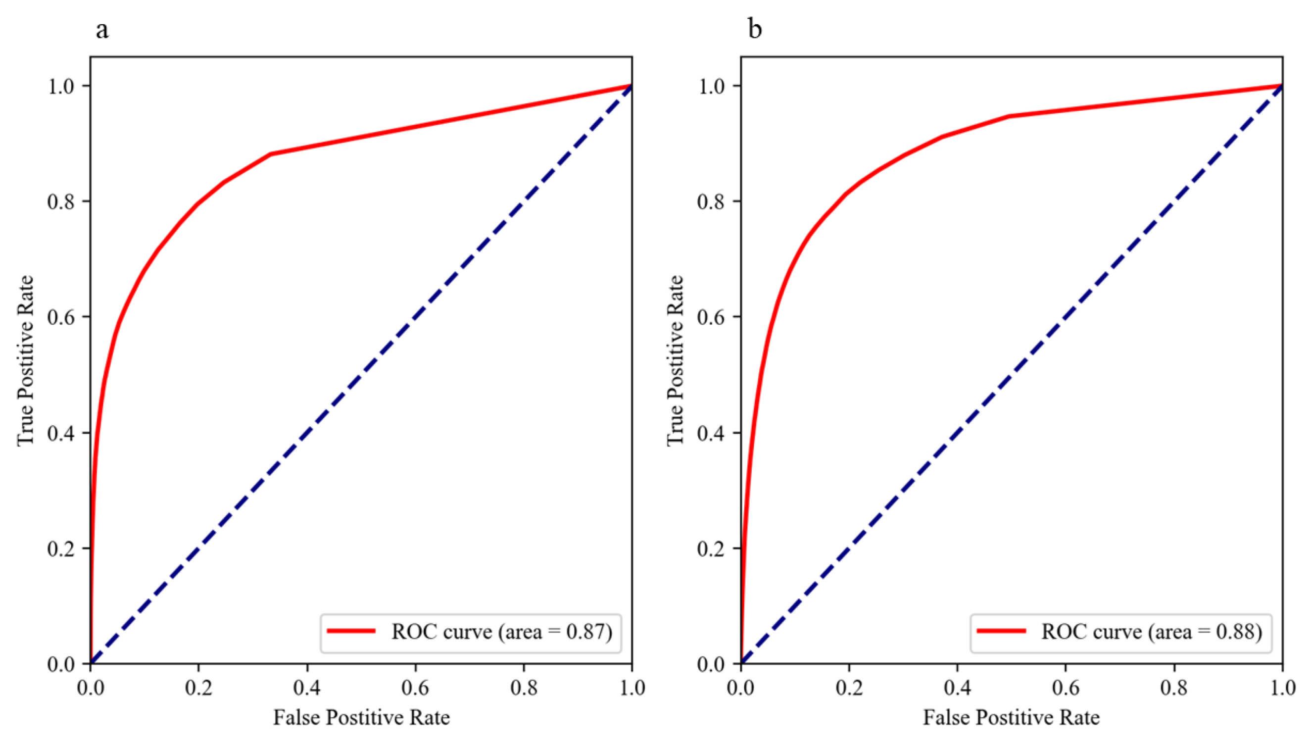
4.2.1. Performance of the Random Forest Algorithm

The ROC curves and corresponding AUCs for urban development probabilities during 2004–2009 and 2009–2016 are shown in Figure 8. The AUC values for these two periods are 0.87 and 0.88, revealing acceptable performance of the RF model in the representation of the local relationship between the driving factors and the urban development probability.

4.2.2. Calibrated Parameters for the Patch-Based CA Model

Table 3 shows the observed mean and variance of patch size for different urban expansion patterns and their corresponding percentages from 2004 to 2016 via 2009. It can be seen that more urban patches were generated through the organic urban development process between 2004 and 2016. Generally, the spontaneous growth process tends to produce smaller urban patches than the organic growth process.
The GA tool tuned the model parameters from the initial values and the solution space was constrained by the defined ranges (as shown in Table 4). The population size of GA was set to 100. Figure 9 shows the convergence process of the GA tool. It shows that the best fitness score in each generation increases from 0.564 to 0.584 and the GA tool stops after evolving for 50 generations. The calibrated model parameters are presented in Table 4. The calibrated organic proportion parameter (0.78) indicates that the urban growth in the study area preferred the compact urban growth pattern, which would improve the connectedness and cohesion of the urban landscape. The isometry parameter shows that the self-growth of new urban patches in both urban growth processes tended to follow an elongated pattern. The corresponding urban land map generated from the CA model using the calibrated parameters (the fitness score is 0.584) is illustrated in Figure 10. Visual inspection shows that there exists a high agreement between the simulated and observed urban land pattern. But the simulated urban patches are more dispersed and fragmented than the observed ones, which means the CA model parameters can be further optimized as needed.

4.2.3. Validation of the Calibrated CA Model

We ran the calibrated CA model 100 times. The simulated urban land map with the highest similarity (0.398) is presented in Figure 11. It can be seen in Figure 11 that the simulated urban pattern matches the observed one well, although patches generated by the CA model are more irregular. Notably, as shown in Figure 11a3,b3, the spontaneous urban growth observed was captured successfully by the CA model, which reveals the that the proposed CA model operates favorably for the representation of the different urban growth patterns. The mean reciprocal similarity for these 100 model runs was 0.389 with a standard deviation of 0.0036, which asserts a good generalization ability of the calibrated CA model. Thus, the CA model is capable of projecting future urban growth with support from the RF algorithm and the GA tool.

4.3. Scenario-Based Delineation of UGBs

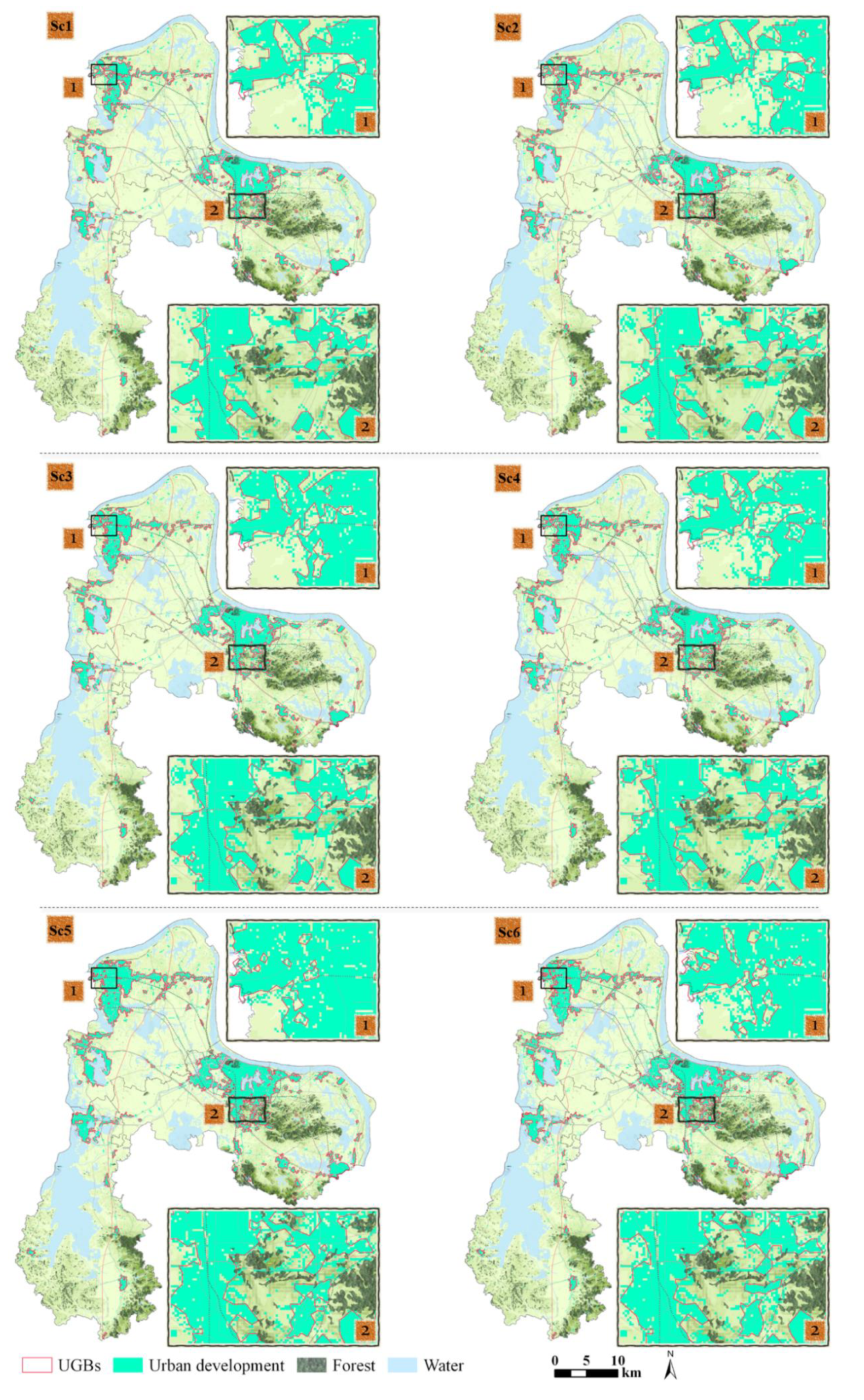
4.3.1. The Simulated Urban Landscape in 2030 under Different Scenarios

The organic proportion parameter of the CA in the compact scenario was assigned value 1 which means no spontaneous growth was allowed, and for the spontaneous scenario, the organic proportion parameter was 0.39 (decreasing the calibrated percentage by 50%). The CA model was implemented under the six scenarios to simulate the urban land patterns in 2030 starting from 2016, using the calibrated model parameters, except for the organic proportion. The model ran 100 times for each scenario and the resulting urban land maps were aggregated. Figure 12 shows the histogram of the urbanization frequency maps under the six scenarios. As can be seen, there is not much difference in the distribution of urbanization frequency between different spatial patterns of urban growth (compact or spontaneous) under the slow and moderate urban growth scenarios. But the difference becomes larger when more land is developed. To be specific, 20% of the total developed cells in scenario 5 (fast urban growth with compact pattern) have urbanization frequencies larger than 90. However, only 8% of the cells have a frequency higher than 90 in scenario 6 (which have the same expected urban demand but follow a dispersed urban growth pattern). In addition, the percentages of cells that have urbanization frequencies smaller than 10 are 27% and 38% for scenario 5 and 6, respectively.
The total area of new urban development and the frequency threshold used to prune the aggregated urbanization map are shown in Table 5. The pruned urban land maps under six scenarios are illustrated in Figure 13. Visual inspection of the pruned urban land maps (Figure 13) also reveals that the distinctness within the simulated urban landscapes between different spatial patterns of urban development increases when more urban land is requested. In addition, landscape metrics for new patches in the pruned urban maps under these scenarios were calculated in the Fragstats software [76] to characterize the spatial pattern of the simulated urban landscape, as shown in Table 6. Detailed descriptions of these landscape metrics can be found in supplementary materials. Results show that the urban patterns are more connected and aggregated in the compact urban growth scenarios. The number of new patches (NP) generated under the compact scenarios is much smaller than that in the spontaneous scenarios. The contiguity (CONTIG) and the cohesion (COHESION) indices suggest that the connectedness of new patches are better in the compact scenarios than in the dispersed ones, and the Euclidean nearest-neighbor (ENN) and the aggregation (AI) indices indicate that new patches are more spatially clustered in the compact scenarios.

4.3.2. Established UGBs from the Simulated Urban Landscapes

The UGBs delineated based on the pruned urban land maps are presented in Figure 14. The results show that the morphological operators worked well in converting the simulated urban land maps into the UGBs. The general shapes of the delineated UGBs show good agreement with the simulated urban distributions. But the difference of UGBs generated under the compact and the spontaneous scenarios with the same urban demand is not as apparent as the original urban land maps due to the effects of the morphological operators. Because many small and dispersed urban patches were removed, and the narrow gaps between patches and the holes within patches were filled by the opening and closing operators, as shown in the sub-areas in Figure 14. Therefore, the area of urban development within the delineated UGBs is less than the predicted urban demands. These area differences are larger in the spontaneous scenarios than that in the compact scenarios, especially when more urban development is expected (as shown in Table 7). For example, the desired urban demand in the fast growth scenarios is 214.77 km2, while the simulated UGBs only encompass 180.28 km2 and 168.87 km2 urban land under the compact and spontaneous growth patterns, respectively. Figure 15 compares the UGBs under the compact and spontaneous patterns in the fast growth scenario (Figure 15a), and the UGBs in the compact scenarios with different urban growth rates were also overlapped to show their spatial disagreement (Figure 15b). It can be seen in Figure 15a that there is high agreement between the UGBs delineated under two urban expansion patterns in the fast growth scenario, despite the removal of small patches and infill of gaps and holes.

5. Discussion

5.1. Feasibility of the Proposed CA Model

Although the simulated urban patches are more dispersed and fragmented than the observed ones in both the calibration and validation processes, which may reveal further improvements in both the CA model parameters and the model structure, the results still verified the applicability of the proposed CA model. Application of the CA model reveals that the spatial parameter for patch layout control impacts the spatial pattern of simulated urban landscapes. The histogram of the aggregated urbanization frequency (Figure 12) suggests that if the urban development process follows a compact pattern; more cells will distribute in the high urbanization frequency intervals, which means a higher spatial agreement among multiple model replications in a scenario. However, the impact of the spatial pattern of patch growing process may be marginal in the early stage of urban development but will become apparent when more land is converted for urban uses. Moreover, the difference of urban land allocation between the two spatial patterns of urban land allocation indicates that a compact urban growth behavior may reduce the uncertainty in terms of the location agreement among model replications. The total area of new urban development and the pruning threshold under different scenarios also supports the findings above. Under the spontaneous growth scenarios (2, 4, and 6), more cells are likely to be developed, which makes the urban growth trajectory more difficult to be predicted. Moreover, the pruning thresholds for the compact growth scenarios (1, 3, and 5) are larger than the spontaneous scenarios (2, 4, and 6), which suggests that candidate cells for future urban development are more spatially aggregated and can lead to more compact urban landscapes. A comparison of the pruned urban land maps under different scenarios also indicates that urban land tends to expand in a more compact manner when more organic growth is preferred.
The model calibration and validation results also reveals an overestimation of organic urban growth and an underestimation of spontaneous urban growth, which is a common issue in CA-based urban growth model due to the embedded neighborhood mechanism. CA models are used to assume that locations adjacent to existing urban areas are tend to show higher potential of future development. this assumption can lead to more organic growth. This is a major reason why we divide urban growth into organic and spontaneous urban growth. The other reason for the overestimation is that patches from the spontaneous growth are agglomerated with patches from organic growth over the process of urban development. Therefore, patches in the final outputs seems to be generated mostly from the organic process.

5.2. Flexibility of the Proposed Framework in Building Scenarios for UGB Delineation

The patch-based CA model proposed, consists of two separate modules: the demand module that allows modelers to specify the quantity of urban growth, and the spatialization module that determines the spatial arrangement of these demands, which provides modelers the ability to control patch characteristics (the patch size and shape parameters) and urban compactness (the organic proportion parameter) [77]. By using this demand-allocation framework, modelers can apply various methods (such as trend interpolation, linear regression, Markov chains, and system dynamics models) [78] and social-economic indicators (such as GDP, population, and immigration) to estimate future urban demand, and therefore, can establish various social-economic scenarios for UGB delineation by the adjustment of these indicators. In this study, we used the linear extrapolation method to forecast future urban demand. However, other sophisticated approaches, such as machine learning and system dynamics models, could be applied to involve more essential social-economic indicators. Additionally, the spatialization module enables the models to build a variety of spatial scenarios by manipulation of the patch characteristics—the urban compactness, the ecological constraints, and even the spatial drivers for the estimation of urban development probability. Therefore, the proposed framework offers the modeler flexibility in building various spatial and nonspatial coupled scenarios for UGB delineation.

5.3. Policy Implications of the UGB Alternatives

The overlapped areas within the two UGBs under the scenarios of fast urban growth are more reliable and reasonable to be included in future urban development because they are insensitive to the spatial patterns of urban growth. The areal agreement between these two scenarios is 131.43 km2, accounting for 72.51% of the merged areas (181.27 km2) of these two UGBs. The disagreements in these UGBs can be reserved as candidate locations where future urban development are very possible under different urban expansion patterns. Thus, further field inspections may be needed in these regions to make sure of their availability for urban development. Similarly, the common areas of UGBs in the slow, moderate, and fast urban growth scenarios with a compact pattern can be considered as the primary locations for future urban allocation. The area of these overlapped regions is 166.55 km2, which accounts for 91.19% of the merged area (182.64 km2) of the three UGBs. The disagreement areas in the slow, moderate, and fast growth scenarios are potential regions that can serve as sequential candidates to be developed in the future. In other words, these disagreements indicate the elastic regions of UGBs [79] under different socio-economic scenarios if the current UGBs are no longer suitable for future urban growth.

6. Conclusions

This study demonstrates that artificial intelligence, such as CA, evolutionary computation, and machine learning, can help decisionmakers capture the complexity of urban development, and thus, make informed decisions in urban management. An application of our proposed framework for UGB delineation in a rapidly growing city in China revealed the applicability and reliability of these artificial intelligence methods in the simulation of urban growth and the delineation of UGBs. The patch-based CA model that represents urban growth as an organic and spontaneous patch-generation processes can simulate a more realistic urban landscape by a coupled consideration of both the spatial process and pattern of urban development. The random forest model can successfully build the relationship between the driving factors and the urban development probability. The key model parameters calibrated through the genetic algorithm capture the landscape characteristics of the historical urban changes well, and thus, can be used for future projections. In addition, the results suggest that empirical knowledge from historical observations can help the genetic algorithm avoid overfitting to some extent. In this study, the prior knowledge of the landscape characteristics was derived using landscape expansion index analysis and was incorporated in the model to constrain the behavior of the genetic algorithm. Thus, the historical trend of urban growth was maintained for future projection. The UGB alternatives under the six spatial and socio-economic scenarios showed that with less urban growth the difference of simulated urban distribution is not that obvious, but when more urban land is budgeted, the disagreement of simulated urban pattern between the compact and spontaneous scenarios becomes significant. Larger patches are generated in the compact scenarios, and these newly-generated patches are more connected and aggregated. Results demonstrate that the spatial compactness of patch allocation can impact the layout of delineated UGBs.
In this study, we only investigate how population growth and the spatial arrangement of urban development impact future UGBs. Although a simple population projection method was applied, and the factors that drives future urban development can be further enhanced, the successful application of the framework in the study area verified the feasibility and flexibility of the proposed framework in incorporation of more sophisticated demand estimation models and more representative spatial drivers that trigger future urban development (such as economic growth, housing demand, investment, and road expansion), which can be a valuable direction of our future work.

Supplementary Materials

The following are available online at https://www.mdpi.com/2071-1050/11/21/6159/s1, Figure S1: title, Table S1: title, Video S1: title.

Author Contributions

Conceptualization, J.Y. and J.G. (Jian Gong); methodology, J.Y., C.L. and Y.S.; validation, J.Y., J.G. (Jian Gong), and W.T.; formal analysis, J.Y. and J.G (Jing Gao).; investigation, J.Y. and Y.S.; resources, C.L. and J.G (Jing Gao).; data curation, J.G (Jing Gao).; writing—original draft preparation, J.Y. and Y.S.; writing—review and editing, J.Y., W.T., C.L. and J.G. (Jian Gong); visualization, J.Y. and Y.S.; supervision, J.G. (Jian Gong) and W.T.; funding acquisition, J.G. (Jian Gong).

Funding

This study was supported by National Social Science Foundation of China (14BJY057); the National Natural Science Foundation of China (41871172); the National Natural Science Foundation of China (number. 41701228); and the Fundamental Research Funds for the Central Universities, China University of Geosciences (GUGL170408).

Acknowledgments

The authors thank Shicheng Li, Cheng Liu, and Jingye Li for their assistance.

Conflicts of Interest

The authors declare no conflict of interest.

References

  1. D’Amour, C.B.; Reitsma, F.; Baiocchi, G.; Barthel, S.; Güneralp, B.; Erb, K.-H.; Haberl, H.; Creutzig, F.; Seto, K.C. Future urban land expansion and implications for global croplands. Proc. Natl. Acad. Sci. USA 2017, 114, 8939–8944. [Google Scholar] [CrossRef] [PubMed]
  2. Newbold, T.; Hudson, L.N.; Arnell, A.P.; Contu, S.; De Palma, A.; Ferrier, S.; Hill, S.L.; Hoskins, A.J.; Lysenko, I.; Phillips, H.R. Has land use pushed terrestrial biodiversity beyond the planetary boundary? A global assessment. Science 2016, 353, 288–291. [Google Scholar] [CrossRef] [PubMed]
  3. Long, Y.; Han, H.; Lai, S.-K.; Mao, Q. Urban growth boundaries of the Beijing Metropolitan Area: Comparison of simulation and artwork. Cities 2013, 31, 337–348. [Google Scholar] [CrossRef]
  4. Ding, C.R.; Knaap, G.J.; Hopkins, L.D. Managing urban growth with urban growth boundaries: A theoretical analysis. J. Urban Econ. 1999, 46, 53–68. [Google Scholar] [CrossRef]
  5. Dempsey, J.A.; Plantinga, A.J. How well do urban growth boundaries contain development? Results for Oregon using a difference-in-difference estimator. Reg. Sci. Urban Econ. 2013, 43, 996–1007. [Google Scholar] [CrossRef]
  6. Hepinstall-Cymerman, J.; Coe, S.; Hutyra, L.R. Urban growth patterns and growth management boundaries in the Central Puget Sound, Washington, 1986–2007. Urban Ecosyst. 2013, 16, 109–129. [Google Scholar] [CrossRef]
  7. Coiacetto, E. Residential sub-market targeting by developers in Brisbane. Urban Policy Res. 2007, 25, 257–274. [Google Scholar] [CrossRef]
  8. Cho, C.-J. The Korean growth-management programs: Issues, problems and possible reforms. Land Use Policy 2002, 19, 13–27. [Google Scholar] [CrossRef]
  9. Gordon, D.; Vipond, S. Gross density and new urbanism: Comparing conventional and new urbanist suburbs in Markham, Ontario. Am. Plan. Assoc. J. Am. Plan. Assoc. 2005, 71, 41. [Google Scholar] [CrossRef]
  10. Venkataraman, M. Analyzing urban growth boundary effects in the city of Bengaluru. IIM Bangalore Res. Paper 2014, 464. [Google Scholar] [CrossRef]
  11. He, Q.; Tan, R.; Gao, Y.; Zhang, M.; Xie, P.; Liu, Y. Modeling urban growth boundary based on the evaluation of the extension potential: A case study of Wuhan city in China. Habitat Int. 2018, 72, 57–65. [Google Scholar] [CrossRef]
  12. Tayyebi, A.; Perry, P.C.; Tayyebi, A.H. Predicting the expansion of an urban boundary using spatial logistic regression and hybrid raster-vector routines with remote sensing and GIS. Int. J. Geogr. Inf. Sci. 2014, 28, 639–659. [Google Scholar] [CrossRef]
  13. Tayyebi, A.; Pijanowski, B.C.; Pekin, B. Two rule-based Urban Growth Boundary Models applied to the Tehran Metropolitan Area, Iran. Appl. Geogr. 2011, 31, 908–918. [Google Scholar] [CrossRef]
  14. Tayyebi, A.; Pijanowski, B.C.; Tayyebi, A.H. An urban growth boundary model using neural networks, GIS and radial parameterization: An application to Tehran, Iran. Landsc. Urban Plan. 2011, 100, 35–44. [Google Scholar] [CrossRef]
  15. Railsback, S.F.; Lytinen, S.L.; Jackson, S.K. Agent-based Simulation Platforms: Review and Development Recommendations. Simulation 2016, 82, 609–623. [Google Scholar] [CrossRef]
  16. Matthews, R.B.; Gilbert, N.G.; Roach, A.; Polhill, J.G.; Gotts, N.M. Agent-based land-use models: A review of applications. Landsc. Ecol. 2007, 22, 1447–1459. [Google Scholar] [CrossRef]
  17. Batty, M. Cities and Complexity: Understanding Cities with Cellular Automata, Agent-Based Models, and Fractals; The MIT Press: Cambridge, MA, USA, 2007. [Google Scholar]
  18. Liang, X.; Liu, X.; Li, X.; Chen, Y.; Tian, H.; Yao, Y. Delineating multi-scenario urban growth boundaries with a CA-based FLUS model and morphological method. Landsc. Urban Plan. 2018, 177, 47–63. [Google Scholar] [CrossRef]
  19. Wu, C.; Pei, F.; Zhou, Y.; Wang, K.; Xu, L. Delineating Urban Growth Boundary from Perspective of “Negative Planning”: A Case Study of the Central Urban District in Xuzhou. Geogr. Geo-Inf. Sci. 2017, 33, 92–98. [Google Scholar]
  20. Ma, S.; Li, X.; Cai, Y. Delimiting the urban growth boundaries with a modified ant colony optimization model. Comput. Environ. Urban Syst. 2017, 62, 146–155. [Google Scholar] [CrossRef]
  21. Moghadam, S.A.; Karimi, M.; Habibi, K. Simulating urban growth in a megalopolitan area using a patch-based cellular automata. Trans. GIS 2018, 22, 249–268. [Google Scholar] [CrossRef]
  22. Li, X.C.; Gong, P.; Yu, L.; Hu, T.Y. A segment derived patch-based logistic cellular automata for urban growth modeling with heuristic rules. Comput. Environ. Urban Syst. 2017, 65, 140–149. [Google Scholar] [CrossRef]
  23. Chen, Y.M.; Li, X.; Liu, X.P.; Ai, B. Modeling urban land-use dynamics in a fast developing city using the modified logistic cellular automaton with a patch-based simulation strategy. Int. J. Geogr. Inf. Sci. 2014, 28, 234–255. [Google Scholar] [CrossRef]
  24. Wang, F.; Marceau, D.J. A Patch-based Cellular Automaton for Simulating Land-use Changes at Fine Spatial Resolution. Trans. GIS 2013, 17, 828–846. [Google Scholar] [CrossRef]
  25. Meentemeyer, R.K.; Tang, W.W.; Dorning, M.A.; Vogler, J.B.; Cunniffe, N.J.; Shoemaker, D.A. FUTURES: Multilevel Simulations of Emerging Urban-Rural Landscape Structure Using a Stochastic Patch-Growing Algorithm. Ann. Assoc. Am. Geogr. 2013, 103, 785–807. [Google Scholar] [CrossRef]
  26. Chen, Y.; Li, X.; Liu, X.; Huang, H.; Ma, S. Simulating urban growth boundaries using a patch-based cellular automaton with economic and ecological constraints. Int. J. Geogr. Inf. Sci. 2019, 33, 55–80. [Google Scholar] [CrossRef]
  27. XIONG, H.-F.; WANG, Y.-H. Spatial variability of soil nutrients in wetland of Liangzi Lake. Plant Nutr. Fertil. Sci. 2005, 5, 002. [Google Scholar]
  28. Li, X.; Yu, X.; Jiang, L.; Li, W.; Liu, Y.; Hou, X. How important are the wetlands in the middle-lower Yangtze River region: An ecosystem service valuation approach. Ecosyst. Serv. 2014, 10, 54–60. [Google Scholar] [CrossRef]
  29. Liu, X.; Zhao, C.; Song, W. Review of the evolution of cultivated land protection policies in the period following China’s reform and liberalization. Land Use Policy 2017, 67, 660–669. [Google Scholar] [CrossRef]
  30. Long, H. Land Use Policy in China: Introduction; Elsevier: Amsterdam, The Netherlands, 2014. [Google Scholar]
  31. Liu, D.; Tang, W.; Liu, Y.; Zhao, X.; He, J. Optimal rural land use allocation in central China: Linking the effect of spatiotemporal patterns and policy interventions. Appl. Geogr. 2017, 86, 165–182. [Google Scholar] [CrossRef]
  32. Huang, X.; Li, Y.; Yu, R.; Zhao, X. Reconsidering the controversial land use policy of “linking the decrease in rural construction land with the increase in urban construction land”: A local government perspective. China Rev. 2014, 14, 175–198. [Google Scholar]
  33. State Council Leading Office of the Second China Land Census. Training Manual of the Second China Land Census; China Agriculture Press: Beijing, China, 2007.
  34. Yao, Y.; Li, X.; Liu, X.; Liu, P.; Liang, Z.; Zhang, J.; Mai, K. Sensing spatial distribution of urban land use by integrating points-of-interest and Google Word2Vec model. Int. J. Geogr. Inf. Sci. 2017, 31, 825–848. [Google Scholar] [CrossRef]
  35. Silverman, B.W. Density Estimation for Statistics and Data Analysis; Routledge: Abingdon, UK, 2018. [Google Scholar]
  36. ESRI, R. ArcGIS Desktop: Release 10; Environmental Systems Research Institute: Redlands, CA, USA, 2011. [Google Scholar]
  37. Li, Y.; Ma, Q.; Song, Y.; Han, H. Bringing conservation priorities into urban growth simulation: An integrated model and applied case study of Hangzhou, China. Resour. Conserv. Recycl. 2019, 140, 324–337. [Google Scholar] [CrossRef]
  38. Mellor, A.; Haywood, A.; Stone, C.; Jones, S. The performance of random forests in an operational setting for large area sclerophyll forest classification. Remote Sens. 2013, 5, 2838–2856. [Google Scholar] [CrossRef]
  39. Kamusoko, C.; Gamba, J. Simulating Urban Growth Using a Random Forest-Cellular Automata (RF-CA) Model. ISPRS Int. J. Geo-Inf. 2015, 4, 447–470. [Google Scholar] [CrossRef]
  40. Breiman, L. Random Forests. Mach. Learn. 2001, 45, 5–32. [Google Scholar] [CrossRef] [Green Version]
  41. Pedregosa, F.; Varoquaux, G.; Gramfort, A.; Michel, V.; Thirion, B.; Grisel, O.; Blondel, M.; Prettenhofer, P.; Weiss, R.; Dubourg, V. Scikit-learn: Machine learning in Python. J. Mach. Learn. Res. 2011, 12, 2825–2830. [Google Scholar]
  42. Gounaridis, D.; Chorianopoulos, I.; Symeonakis, E.; Koukoulas, S. A Random Forest-Cellular Automata modelling approach to explore future land use/cover change in Attica (Greece), under different socio-economic realities and scales. Sci. Total Environ. 2019, 646, 320–335. [Google Scholar] [CrossRef]
  43. Mas, J.-F.; Soares Filho, B.; Pontius, R.; Farfán Gutiérrez, M.; Rodrigues, H. A suite of tools for ROC analysis of spatial models. ISPRS Int. J. Geo-Inf. 2013, 2, 869–887. [Google Scholar] [CrossRef]
  44. Liu, X.; Li, X.; Chen, Y.; Tan, Z.; Li, S.; Ai, B. A new landscape index for quantifying urban expansion using multi-temporal remotely sensed data. Landsc. Ecol. 2010, 25, 671–682. [Google Scholar] [CrossRef]
  45. Soares-Filho, B.S.; Cerqueira, G.C.; Pennachin, C.L. DINAMICA—A stochastic cellular automata model designed to simulate the landscape dynamics in an Amazonian colonization frontier. Ecol. Model. 2002, 154, 217–235. [Google Scholar] [CrossRef]
  46. Soares-Filho, B.S.; Rodrigues, H.O.; Costa, W. Modeling Environmental Dynamics with Dinamica EGO; Centro de Sensoriamento Remoto; Universidade Federal de Minas Gerais: Belo Horizonte, Minas Gerais, Brazil, 2009; Volume 115. [Google Scholar]
  47. Yang, J.; Gong, J.; Tang, W.; Liu, C. Patch-based cellular automata model of urban growth simulation: Integrating feedback between quantitative composition and spatial configuration. Comput. Environ. Urban Syst. 2020, 79, 101402. [Google Scholar] [CrossRef]
  48. Wang, Q. Using genetic algorithms to optimise model parameters. Environ. Model. Softw. 1997, 12, 27–34. [Google Scholar] [CrossRef]
  49. Holland, J.H. Adaptation in Natural and Artificial Systems: An Introductory Analysis with Applications to Biology, Control, and Artificial Intelligence; MIT Press: Cambridge, MA, USA, 1992. [Google Scholar]
  50. Mitchell, M. An Introduction to Genetic Algorithms; MIT Press: Cambridge, MA, USA, 1998. [Google Scholar]
  51. Cantú-Paz, E. A Summary of Research on Parallel Genetic Algorithms; Technical Report 95007; University of Illinois at Urbana-Champaign: Champaign, IL, USA, 19 July 1995. [Google Scholar]
  52. Konak, A.; Coit, D.W.; Smith, A.E. Multi-objective optimization using genetic algorithms: A tutorial. Reliab. Eng. Syst. Saf. 2006, 91, 992–1007. [Google Scholar] [CrossRef]
  53. Goldberg, D.E.; Deb, K.; Clark, J.H. Genetic algorithms, noise, and the sizing of populations. Complex Syst. 1992, 6, 333–362. [Google Scholar]
  54. Chatterjee, S.; Laudato, M.; Lynch, L.A. Genetic algorithms and their statistical applications: An introduction. Comput. Stat. Data Anal. 1996, 22, 633–651. [Google Scholar] [CrossRef]
  55. Miller, B.L.; Goldberg, D.E. Genetic algorithms, selection schemes, and the varying effects of noise. Evol. Comput. 1996, 4, 113–131. [Google Scholar] [CrossRef]
  56. Forrest, S. Genetic algorithms. ACM Comput. Surv. 1996, 28, 77–80. [Google Scholar] [CrossRef]
  57. Keijzer, M.; Merelo, J.J.; Romero, G.; Schoenauer, M. Evolving objects: A general purpose evolutionary computation library. In Artificial Evolution 5th International Conference, Evolution Artificielle, EA 2001, Le Creusot, France, 29–31 October 2001, Selected Papers; Springer: Berlin/Heidelberg, Germany, 2001; pp. 231–242. [Google Scholar]
  58. Soares-Filho, B.; Rodrigues, H.; Follador, M. A hybrid analytical-heuristic method for calibrating land-use change models. Environ. Model. Softw. 2013, 43, 80–87. [Google Scholar] [CrossRef]
  59. Ong, Y.S.; Nair, P.B.; Keane, A.J. Evolutionary optimization of computationally expensive problems via surrogate modeling. AIAA J. 2003, 41, 687–696. [Google Scholar] [CrossRef]
  60. Liu, Y.; Khu, S.-T. In Automatic calibration of numerical models using fast optimisation by fitness approximation. In Proceedings of the 2007 International Joint Conference on Neural Networks, Orlando, FL, USA, 12–17 August 2007; pp. 1073–1078. [Google Scholar]
  61. Fix, E.; Hodges, J.L., Jr. Discriminatory Analysis-Nonparametric Discrimination: Consistency Properties; California Univ Berkeley: Berkeley, CA, USA, 1951. [Google Scholar]
  62. Mollineda, R.A.; Ferri, F.J.; Vidal, E. An efficient prototype merging strategy for the condensed 1-NN rule through class-conditional hierarchical clustering. Pattern Recognit. 2002, 35, 2771–2782. [Google Scholar] [CrossRef]
  63. Vliet, J.V.; Bregt, A.; Brown, D.G.; Delden, H.V.; Heckbert, S.; Verburg, P.H. A review of current calibration and validation practices in land-change modeling. Environ. Model. Softw. 2016, 82, 174–182. [Google Scholar] [CrossRef]
  64. Costanza, R. Model goodness of fit: A multiple resolution procedure. Ecol. Model. 1989, 47, 199–215. [Google Scholar] [CrossRef]
  65. Power, C.; Simms, A.; White, R. Hierarchical fuzzy pattern matching for the regional comparison of land use maps. Int. J. Geogr. Inf. Sci. 2001, 15, 77–100. [Google Scholar] [CrossRef] [Green Version]
  66. Van Vliet, J.; Bregt, A.K.; Hagen-Zanker, A. Revisiting Kappa to account for change in the accuracy assessment of land-use change models. Ecol. Model. 2011, 222, 1367–1375. [Google Scholar] [CrossRef]
  67. Hagen, A. Fuzzy set approach to assessing similarity of categorical maps. Int. J. Geogr. Inf. Syst. 2003, 17, 235–249. [Google Scholar] [CrossRef] [Green Version]
  68. Almeida, C.M.; Gleriani, J.M.; Castejon, E.F.; Soares-Filho, B.S. Using neural networks and cellular automata for modelling intra-urban land-use dynamics. Int. J. Geogr. Inf. Sci. 2008, 22, 943–963. [Google Scholar] [CrossRef]
  69. Banister, J.; Bloom, D.E.; Rosenberg, L. Population aging and economic growth in China. In The Chinese Economy; Palgrave Macmillan: London, UK, 2012; pp. 114–149. [Google Scholar]
  70. Fong, V.L. Only Hope: Coming of Age under China’s One-Child Policy; Stanford University Press: Palo Alto, CA, USA, 2004. [Google Scholar]
  71. Hesketh, T.; Zhou, X.; Wang, Y. The end of the one-child policy: Lasting implications for China. JAMA 2015, 314, 2619–2620. [Google Scholar] [CrossRef]
  72. Zeng, Y.; Hesketh, T. The effects of China’s universal two-child policy. Lancet 2016, 388, 1930–1938. [Google Scholar] [CrossRef]
  73. Chen, Y.; Liu, X.; Li, X. Calibrating a Land Parcel Cellular Automaton (LP-CA) for urban growth simulation based on ensemble learning. Int. J. Geogr. Inf. Sci. 2017, 31, 2480–2504. [Google Scholar] [CrossRef]
  74. Narayanan, A. Fast binary dilation/erosion algorithm using kernel subdivision. In Asian Conference on Computer Vision, Hyderabad, India, 13–16 January 2006; Springer: Berlin/Heidelberg, Germany, 2006; pp. 335–342. [Google Scholar]
  75. Zhou, R.; Zhang, H.; Ye, X.-Y.; Wang, X.-J.; Su, H.-L. The Delimitation of Urban Growth Boundaries Using the CLUE-S Land-Use Change Model: Study on Xinzhuang Town, Changshu City, China. Sustainability 2016, 8, 1182. [Google Scholar] [CrossRef]
  76. McGarigal, L.; Marks, B. FRAGSTATS: Spatial pattern analysis program for quantifying landscape structure. In General Technical Report PNW-GTR-351; U.S. Department of Agriculture, Forest Service, Pacific Northwest Research Station: Portland, OR, USA, 1995; p. 122. [Google Scholar]
  77. White, R.; Engelen, G. Cellular automata and fractal urban form: A cellular modelling approach to the evolution of urban land-use patterns. Environ. Plan. A 1993, 25, 1175–1199. [Google Scholar] [CrossRef]
  78. Brown, D.G.; Verburg, P.H.; Pontius, R.G., Jr.; Lange, M.D. Opportunities to improve impact, integration, and evaluation of land change models. Curr. Opin. Environ. Sustain. 2013, 5, 452–457. [Google Scholar] [CrossRef]
  79. Cho, S.-H.; Poudyal, N.; Lambert, D.M. Estimating spatially varying effects of urban growth boundaries on land development and land value. Land Use Policy 2008, 25, 320–329. [Google Scholar] [CrossRef]
Figure 1. Location of the study area.
Sustainability 11 06159 g001
Figure 2. Land use/cover maps. (a) 2004, (b) 2009, and (c) 2016. Land use/cover maps were produced by the local government using a human–computer interaction method based on the Landsat and SPOT satellite images.
Sustainability 11 06159 g002
Figure 3. Ecologically protected areas in the study area.
Sustainability 11 06159 g003
Figure 4. The framework of urban growth boundaries’ delineation (UGB: urban growth boundary).
Sustainability 11 06159 g004
Figure 5. Workflow of the random forest algorithm.
Sustainability 11 06159 g005
Figure 6. Patch generation function based on seeding and self-growing (adapted from [47]; this figure shows the procedure of generating an urban patch with a size of 3 cells).
Sustainability 11 06159 g006
Figure 7. Population and the fitted trend lines at different time intervals from 1978 to 2016.
Sustainability 11 06159 g007
Figure 8. Relative operating characteristics (ROCs) and areas under the curves (AUCs) for the random forest models. (a) 2004–2009; (b) 2009–2016.
Sustainability 11 06159 g008
Figure 9. Best fitness score in each generation of the genetic algorithm.
Sustainability 11 06159 g009
Figure 10. Simulated and observed urban land map in 2009. (a) Observed urban land map; (b) Simulated urban land map corresponding to the solution with the highest fitness score in the genetic algorithm.
Sustainability 11 06159 g010
Figure 11. Simulated urban land map with the highest fitness score in the 100 model runs and the observed urban land map in 2016. (a) Observed urban land map; (b) simulated urban land map with the highest fitness score.
Sustainability 11 06159 g011
Figure 12. Frequency of urbanization in the aggregated urban map under different scenarios. (Sc1) slow urban growth with a compact spatial pattern; (Sc2) slow urban growth with a dispersed spatial pattern; (Sc3) moderate urban growth with a compact spatial pattern; (Sc4) moderate urban growth with a dispersed spatial pattern; (Sc5) fast urban growth with a compact spatial pattern; (Sc6) fast urban growth with a dispersed spatial pattern.
Sustainability 11 06159 g012
Figure 13. Pruned urban maps under the six scenarios. (Sc1) slow urban growth with a compact spatial pattern; (Sc2) slow urban growth with a dispersed spatial pattern; (Sc3) moderate urban growth with a compact spatial pattern; (Sc4) moderate urban growth with a dispersed spatial pattern; (Sc5) fast urban growth with a compact spatial pattern; (Sc6) fast urban growth with a dispersed spatial pattern.
Sustainability 11 06159 g013
Figure 14. Map of UGBs under different scenarios (UGBs: urban growth boundaries).
Sustainability 11 06159 g014
Figure 15. Comparison maps of UGBs under different scenarios. (a) UGBs under the compact and spontaneous patterns in the fast scenarios of urban growth; (b) UGBs in the compact scenarios with different urban growth rates. UGBs: urban growth boundaries.
Sustainability 11 06159 g015
Table 1. Fitted extrapolation functions and the projected population in 2030.
Population Growth ScenarioFitted Extrapolation FunctionGoodness-Of-Fit (R2)Population in 2030
Lowy = 5,313.62x + 9,598,543.390.971,188,105.41
Moderatey = 10,292.59x + 19,587,739.780.931,306,217.92
Fasty = 15,796.83x + 30,526,304.240.991,541,260.66
Table 2. Per-capita urban land requirement and the projected total urban demands in 2030 under different scenarios.
Population Growth ScenarioPer Capita Urban Demand (The Reference Year)55.49 m2 (2004)96.23 m2 (2009)139.35 m2 (2016)
LowProjected total urban demands (km2)65.92114.33165.56
Moderate72.48125.69182.02
High85.52148.31214.77
Table 3. Observed mean and variance of patch size for different urban expansion patterns and their percentages (cells).
Urban Growth ProcessOrganicSpontaneous
Urban Expansion PatternInfilling and Edge-ExpansionOutlying
urban development Period2004–2009Percentage0.660.34
Mean11.732.13
Variance66.923.12
2009–2016Percentage0.610.39
Mean7.547.63
Variance45.2426.16
2004–2016Percentage0.760.24
Mean25.584.84
Variance196.5619.99
Table 4. Initial values, ranges, and the optimized solutions for the model parameters (cells).
ParametersInitial ValueRangeCalibrated Value
Organic proportion0.69(0, 1)0.78
Patch size and shapeOrganic growthMean 16.56(7.54, 25.58)14.61
Variance120.90(45. 24, 196.56)120.89
Isometry1.00(0, 2)0.57
Spontaneous growthMean4.88(2.13, 7.63)2.47
Variance19.99(3.12, 26.169)7.25
Isometry1.00(0, 2)0.30
Table 5. The amount of newly generated urban patches and the pruning threshold for the aggregated urbanization map in different scenarios.
ScenarioArea of New Urban Development (km2)Pruning Threshold of Urbanization Frequency
Sc1104.7658
Sc2135.6347
Sc3120.3244
Sc4156.1640
Sc5154.1357
Sc6203.8150
Table 6. Landscape metrics of the pruned urban land maps in different scenarios.
Landscape MetricsSc1Sc2Sc3Sc4Sc5Sc6Definition
NP293.00551.00483.00870.00639.001541.00Number of urban patches
CONTIG0.200.130.230.180.260.18Indication of the spatial contiguity of cells within an urban patch
ENN237.07235.04207.05224.57176.67205.19Quantification of patch isolation degree based on the Euclidean nearest-neighbor distances between urban patches
COHESION79.0372.6885.9980.8591.1286.25Measurement of the spatial connectedness of all the urban patches
AI40.4933.6649.7143.7259.2951.77Measurement of the adjacencies or aggregation between the urban patches
Table 7. Area of UGBs under different scenarios (km2).
ScenarioExpectedSimulatedDifference
CompactSpontaneousCompactSpontaneous
Slow165.56132.43129.6933.1335.88
Moderate182.02148.14142.6933.8839.33
Fast214.77180.28168.8734.5045.90

