Article

An Assessment of the Environmental Sustainability and Circularity of Future Scenarios of the Copper Life Cycle in the U.S.

by
Miranda R. Gorman
* and
David A. Dzombak
Civil and Environmental Engineering, Carnegie Mellon University, 119 Porter Hall, 5000 Forbes Ave, Pittsburgh, PA 15213, USA
*
Author to whom correspondence should be addressed.
Sustainability 2019, 11(20), 5624; https://doi.org/10.3390/su11205624
Submission received: 13 September 2019 / Revised: 30 September 2019 / Accepted: 8 October 2019 / Published: 12 October 2019
(This article belongs to the Special Issue Life Cycle Assessment, a Tool for Sustainability and Circular Economy)

Abstract

:
Assessments of availability and sustainability of metals necessary for economic development into the future are important for planning by producers, consumers, and governments. This work assessed the U.S. copper life cycle and examined six future scenarios by which to assess the circular economy and sustainability of copper to 2030. Regression analysis methodology was used to identify relationships among seven drivers and eight materials flows. These relationships were used to develop six forecasts of future scenarios for U.S. production, consumption, old scrap collection, new scrap recovery, landfilling, and scrap exports of copper. Flow forecasts were used to quantify circularity and environmental footprint metrics to assess sustainability. Results of the scenario analyses provide insights into the types of behaviors and trends that could be incentivized to allow for increased circularity of copper. One such finding was that slow population growth and high urbanization resulted in the most circular scenario. Major limitations to circularity are import reliance and scrap exports. Analysis of the scenarios leads to the conclusions that population dynamics are critical to the circularity of copper, as well as that both environmental footprint metrics and circularity indicators must be considered when assessing environmental sustainability.

1. Introduction

Copper is among the most important metals in the U.S. due to its widespread use in the economy in large amounts in both commercial and residential sectors. The economic value of the copper metal is driven by its unique properties and wide range of applications. The growth in demand for copper globally, coupled with environmental impacts of extraction and processing, speak to the need for assessment of the life cycle of the material and its circularity, so that reserves may be prolonged and the embedded energy and environmental footprint of copper may be improved [1]. Several research studies have attempted to assess the criticality of future demand for materials generally [2,3] metals [4], and even specifically copper [5,6,7,8], but such assessments typically do not take into account the relevance of circularity and the circular economy, focusing mostly on the front-end of the material life cycle and not assessing end-of-life (EoL) and scrap flows which play a major role in meeting demand and material availability. Previous works differ from this study in that their time frame of forecasts tend to be shorter term, or the scope of the forecast did not include a complete material life cycle, but only a subset of the entire material life. For example, one study, which analyzed 75 years of data to make long-term projections of material stocks focused on the accumulation of all materials in only the use phase in both the U.S. and Japan [2]. In contrast, the present study focused on the complete life cycle of a single material. Another study, by Schandl et al. focused on production and consumption of materials, but in larger regions [3], which may be problematic in that trends have been shown to vary dramatically even within a region depending on economic development [1]. Existing studies specific to copper include a long-term forecast for the U.S. focused only on the front end of material life cycle [5], a long-term outlook for intensity of use and in-use stocks that is global in focus with general regional breakdowns [6], a global outlook of supply and demand, nonspecific to the U.S. [7], as well as a forecast for global and U.S. copper, but only of production [8]. There is a need for regionally high-resolution analyses of complete life cycles of specific materials.
This study investigated prospects for circularity in the future (up to 2030) by forecasting material flows including production, use, and recovery of copper in the U.S. An assessment of the environmental footprint associated with the projected primary and secondary copper production was also performed. Material demand patterns generally have been studied since the 1950s, and socio-economic theories have predicted “dematerialization” or “decoupling” of material consumption from economic growth and development for several decades [3,9,10,11], though the predicted absolute decrease in material consumption has not been observed at the scale of the national economy [12]. However, starting around the year 2000, copper consumption, both absolute and per capita, and from both primary and secondary copper sources, in the U.S. has declined steadily following steady growth throughout the 20th century [13]. In the development of material flow forecasts, therefore, inclusion of indicators that represent dematerialization or decoupling, which can be represented by material efficiency measurements [14], was done and potential implications for the copper circular economy into the future were considered.

2. Materials and Methods

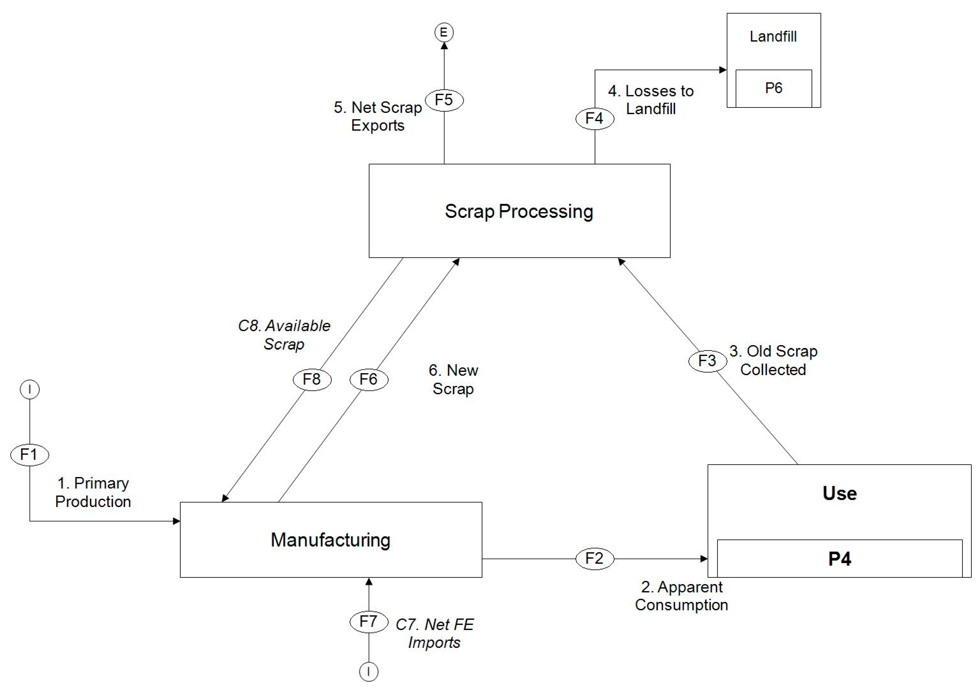
2.1. Modeling Approach

Future (up to 2030) copper production, use, and recovery were forecast using a regression model constructed with parameters that influence the copper life cycle. These forecast scenarios are referred to as Future Scenarios, or FS# throughout this work, all of which consist of forecasts of eight major life cycle flows, six of which are independently forecast, and are referred to as Flows F1–F6, and two of which are calculated using mass balance formulae, referred to as C7 and C8. The first step in developing these forecasts involved use of primary data from a complete stocks and flow analysis for the copper life cycle in the U.S. [1,15] These data, which include historical data for all eight flows from 1970 to 2015 (available in Table SI−2), were employed for determination of regression parameter values. The scale of data (annual data for just 45 years) lends itself to a regression analysis rather than methods that may be more applicable to larger data sets, such as learning algorithms. Multivariate regressions have been used to identify correlations between explanatory variables, referred to in this analysis as “drivers”, and materials flows in existing works globally for materials categories [11], as well as for individual commodities on the national [16] and regional scale [12]. This approach also has been demonstrated to be an effective method for predictive analysis for individual commodities [5,7]. These studies include arguments for the use of linear modeling of copper specifically, as well as of commodities generally, based on global development variables in the absence of a definitive finding of specific nonlinear relationships [7].
Several of the copper material flows examined showed abrupt changes in their historical trends, visible in Figure 1, which depicts the historical data series for the six flows which were used to forecast Flows F1–F6. Apparent consumption and primary production, for example, both show generally increasing trends for the first three decades and then a sharp decline. Net scrap exports follow a relatively flat, or very slowly increasing, trend in the same initial 30 year time period, and then a steep increase beginning around 2000. For this reason, piecewise regression analyses were performed for all flows for two time periods, 1970–2000 and 2000–2015, and material flow forecasts were developed based on the second, more recent time period since it is the most recent trends that are likely to continue. Piecewise linear regressions have been shown to be useful for time series data that show changing trends [17,18].
The piecewise linear regression was performed using several drivers of copper demand, which are shown in Table 1, with sources of the driver variables indicated. Data series for the same 1970–2015 timeframe of the materials flow data were collected for six drivers and time (available in Table SI−1). Time is included in the analysis to represent linearity in the regression, and to capture the linear trend of many of the material flows, as well as to represent trends over time that may not be easily represented by quantitative values, such as substitution or policy changes, similar to the approach of Elshkaki et al. [7]. Published projections available for some of these drivers to 2030 were also collected and are also shown in Table 1 (complete data series are available in Table SI−3). If a published projection was unavailable, as was the case for the contribution of the manufacturing to GDP (Mfg%) and for domestic materials consumption (DMC), a linear projection for the driver to 2030 was employed. Both Mfg% and DMC show highly linear trends, as indicated in Figure 2, and were therefore able to be linearly projected to 2030. Socio-economic demand drivers were considered (GDP, population, and urbanization) as well as material specific drivers (copper price) and finally materials use indicators to represent dematerialization and decoupling (DMC and Mfg%). Any potential derived variables, such as materials intensity (DMC/GDP) or GDP per capita, were not included as potential drivers in the analysis to avoid data redundancy in the model.

2.2. Base Case Scenario Methodology

A base case forecast, or Future Scenario 1 (FS1), was made for 2016–2030 based on the seven drivers and their projected values (from sources indicated in Table 1), for eight major materials flows labeled F1–F8 in the complete copper life cycle, shown in Figure 3. This forecast provides insight into the most likely trends in these major material flows (primary production, apparent consumption, end-of-life collection, landfilling, scrap exports, new scrap recovery, imports, and available scrap) to 2030. A range of other potential future scenarios was considered through the development of five additional forecasts (FS2–6); the development of these are described in Section 2.3.
Regression analysis was performed on major life cycle flows F1–F6, shown in Figure 2, against the drivers listed in Table 1. In order to account for non-linear relationships between dependent (material flows) and independent (drivers) variables, all data were logarithmically transformed, and then quantile–quantile (Q–Q) plots, as introduced by Lorenz [28], were used as one of the most established methods to check the assumption of multivariate normality [29]. The results are presented in Supplemental Information (Figure SI-1 and Table SI-4). Piecewise linear regressions were then performed on these logarithmically transformed raw data, since the transformed data meets linear regression requirements and assumptions. Each material flow F1–F6 was regressed against all seven drivers in an iterative manner to determine which drivers contributed in a meaningful way to the trends exhibited by the material flow. The p-value, which tests the null hypothesis, was used to assess driver influence. p-values above the standard rejection threshold of 0.05 indicate low correlation, or that changes in the driver are not meaningfully associated with changes in the dependent variable, material flow. Drivers with p-values higher than 0.05 were eliminated one by one until a relationship was established with all remaining drivers having a significant effect on the material flow. Material Flows 1–6 (Figure 3) (primary production, apparent consumption, end-of-life collection, scrap landfilled, scrap exported, and new scrap recovery) were forecast using the results of the second interval of the regression analysis based on the historical values (2000–2015). The general form of the resulting regression equation for each piece of the piecewise linear regression can be expressed as:
l n ( F 1 6 ) =   α +   j β j l n ( X j )
where Xj is drivers, F1–6 are material flows, α and β j are transformed coefficients, and j is the number of drivers with valid p-values. The overall quality of this regression can then be evaluated by the R2 value, which indicates goodness-of-fit of the overall modeled result to the observed data. The results of these regressions and values of coefficients as well as R2 values are reported the results (Section 3.1).
Material flows C7 (Front End Imports) and C8 (Available Scrap) are labeled as such in Figure 3. These flows were not independently forecast, but were calculated using mass balance as given in Equation (2). The in-use stock accumulation was also calculated using a mass balance formula, Equation (3).
C 7 , 8 =   Σ F i n Σ F o u t
Δ S t o c k y e a r =   Σ F i n ,   y e a r Σ F o u t , y e a r
Front end imports, here defined as net imports of unrefined, refined, and semi-manufactured copper, were calculated based on mass balance formulae instead of independently forecast, because it is necessary to import (or export in the unlikely event of a surplus of primary production) enough copper to meet demand, represented by apparent consumption (F2 in Figure 3), that cannot be met by the primary production capacity of U.S. mining operations. Available scrap was also calculated instead of forecast because it is one potential representation of future circularity in that it is the predicted remaining scrap that is collected from end-of-life as well as new scrap recovered from manufacturers that is neither landfilled nor exported. This metric “available scrap” as such additionally does not have a representative data series currently, and therefore cannot be forecast from primary data, but must be calculated by mass balance.
The calculated stock and flows were synthesized with all forecasted flows in the framework shown in Figure 3 to represent the entire predicted life cycle of copper in the U.S. to the year 2030.
In order to develop a range of forecasts beyond the base case a scenario analysis approach was used. The scenarios are summarized in Table 2. Two general future scenarios (FS), slower driver change (FS2) and faster driver change (FS3), were developed as bounding cases compared to the base case scenario (FS1). Three additional scenarios (FS4–6) were developed based on results of the base case scenario and used to explore more circular and sustainable future scenarios. All five of these future scenarios were developed using the base case regression equations employed for FS1 but using variability in projections of the drivers used to calculate material flows.

2.3. Scenario Analysis Methodology

In order to develop a range of forecasts beyond the base case, a scenario analysis approach was used. The scenarios are summarized in Table 2. Two general future scenarios (FS), slower driver change (FS2) and faster driver change (FS3), were developed as bounding cases compared to the base case scenario (FS1). Three additional scenarios (FS4–6) were developed based on the results of the base case scenario and used to explore more circular and sustainable future scenarios. All five of these future scenarios were developed using the base case regression equations employed for FS1 but using variability in projections of the drivers used to calculate material flows.
Reported projections for these drivers were identified from available sources, listed in Table 3, when possible. For example, in the case of GDP, the U.S. Department of Agriculture projection [25] was used as a high-end value and an OECD (Organization for Economic Co-operation and Development) projection [30] that had a slightly slower growth rate was used as a low-end value. Population similarly has high and low rate-of-change projections developed by the UN Population Division [31]. For the drivers without published projections, manufacturing contribution to GDP (Mfg%), urbanization, and domestic materials consumption (DMC), the 95% confidence intervals of the linear regressions used for the expected projection were used as high and low values. Copper price was not varied in these scenarios because of a lack of alternate sources from the World Bank commodity forecast. Commodity prices can be highly volatile, so the development of another scenario would be primarily speculation.
The first two scenarios considered outside of the base case forecast scenario (FS1) were the slower driver change (FS2) and faster driver change (FS3) forecasts, developed based on the estimated high- and low-range projections of drivers to identify high and low bounds for forecasted copper stocks and flows up to 2030. The development of these bounding scenarios was based on the general ebb and flow of the material and socioeconomic drivers. In the case that some externality spurs one driver to accelerate and change outside of the expected projection (in Table 1) the others would follow. Scenario FS2 is the slower driver change scenario in which population growth, urbanization, and total GDP all increase in a low-growth scenario, and the decreasing drivers Mfg% and DMC decrease more slowly than the expected projection. Scenario FS3 is the inverse, where population, urbanization, and GDP grow at their maximum projected rates, and Mfg% and DMC decline at the maximum rate.
Three additional scenarios (FS4–6) were also developed with different assumptions relative to the base case. These included a slow population growth but high migration scenario in which population changes more slowly than expected but urbanization changes faster than expected, referred to as FS4, or population migration. Additionally, there was an economic transition scenario, FS5, where GDP grows faster than expected but the contribution of the manufacturing industry declines more slowly than expected. The inverse was considered in FS6, economic stagnation, where GDP grows more slowly but the contribution of manufacturing declines at a faster pace. All these future scenarios, including the base case, and the specific driver projections used to develop them are summarized in Table 2.

3. Results

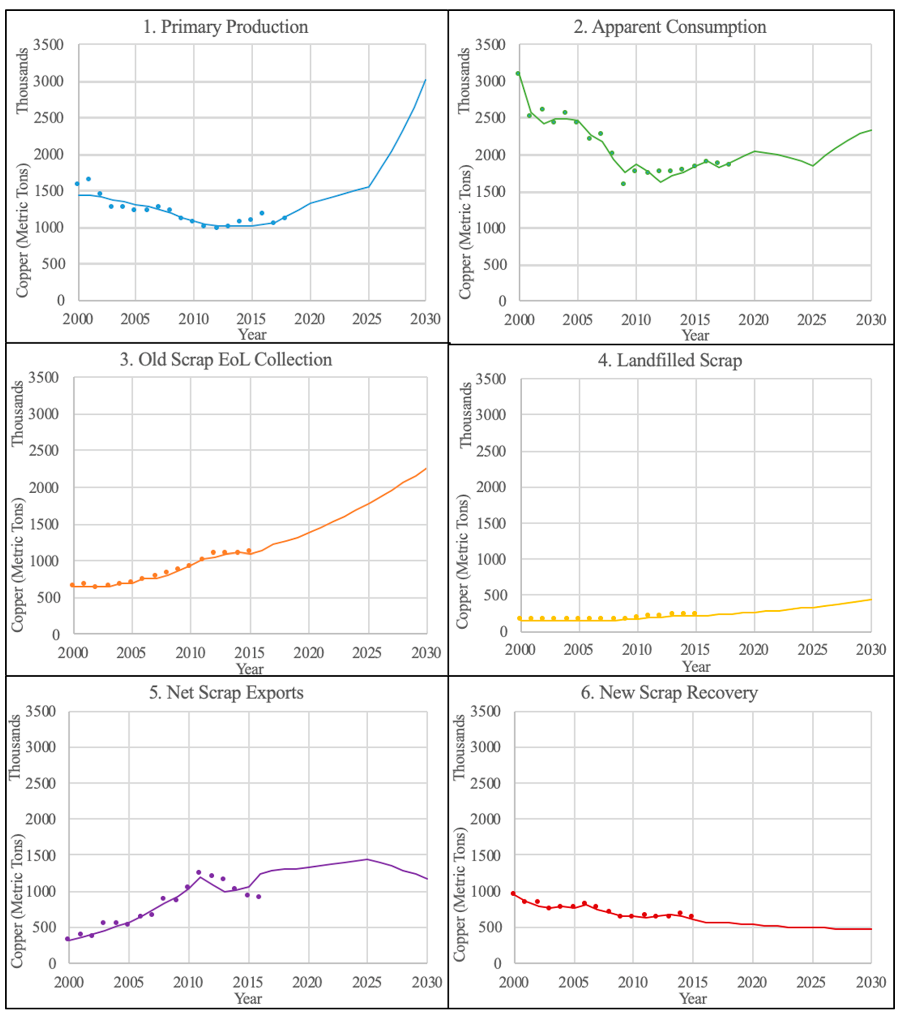
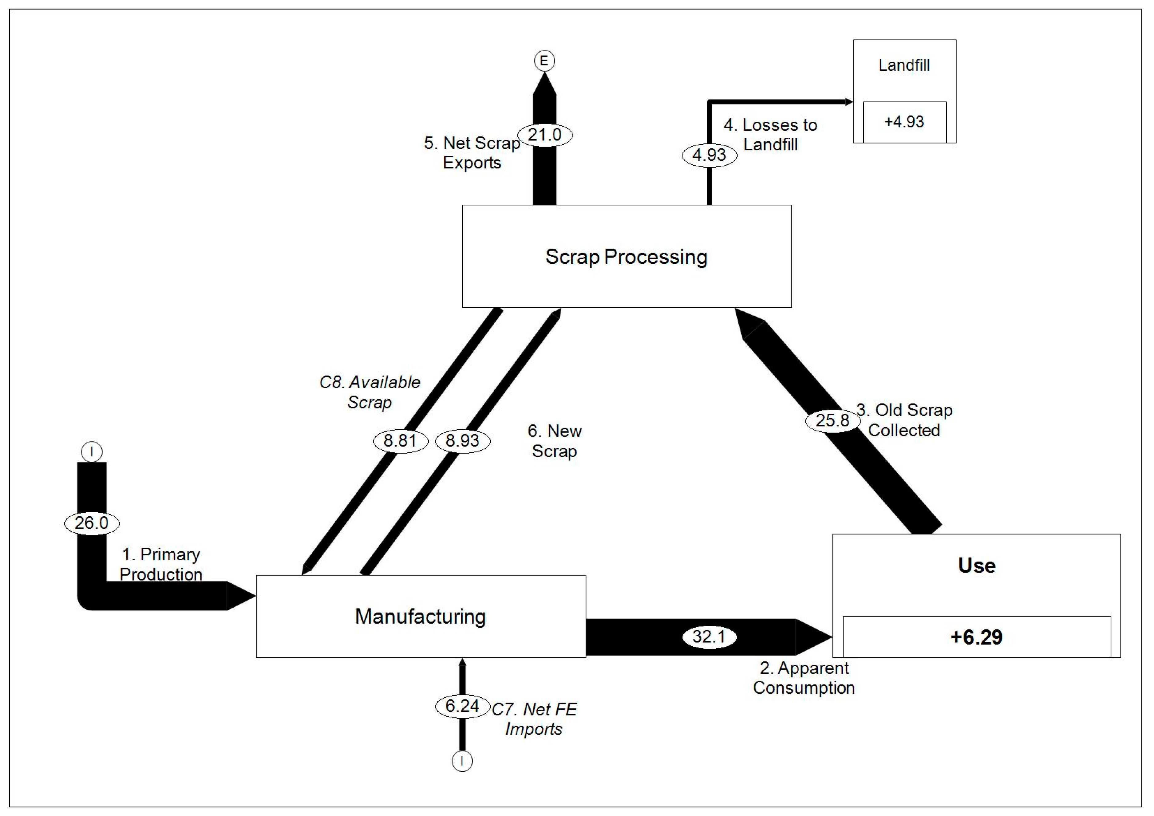
3.1. Base Case (FS1) Scenario Results

Table 4 shows the results of the regression modeling for all six of the major material flows for copper in the U.S. for FS1, the base case forecast scenario. The intercept α as well as the coefficients βj for each driver found to have a significant impact on flow are summarized and can be used in conjunction with Equation (1) to reconstruct the complete equations for each flow. Primary production, in any year t, for example, would be as follows:
ln ( Y 1 , t ) =   6730 +   221 ln ( U r b a n i z a t i o n t ) 1010 ln ( Y e a r t )
Drivers that exhibited negative correlations (β < 0) with flows are shown in red, whereas drivers with positive correlations (β > 0) are shown in green. The modeled material flow forecasts resulting from these relationships as well as observed historical data are presented in Figure 4. Data series for these results can be found in the Supplemental Information (Table SI-5). Forecasts are made for years 2015–2030, though there are observed data for years 1970–2015, the modeled data for 2015 serve as a check against observed data in that same year as well as a baseline for the other scenario analyses.
The results also show a significant increase in production to 2030 (mirrored by increasing end-of-life collection). These forecasts were made based on material flow relationships with drivers, and no technological or physical limitations were imposed upon the model outcome (such as potential shortages) since current U.S. reserves are vast, and technology only continues to improve to extract more difficult resources. For these reasons, the model was constructed to represent market trends and demand without physical limitations to extraction.
The regression modeling for base case scenario FS1 provided insight into the influence that each individual driver has on the overall life cycle of copper. Population dynamics, for example, were found to be a significant driver in five of the six material flows. The only aspect of the copper life cycle that either population or urbanization do not directly affect is end-of-life collection. Urbanization was found to be positively correlated with the front end of the life cycle (primary production and apparent consumption) and negatively correlated with the back-end activities scrap exports. A steady increase or even acceleration of urbanization in the U.S. would therefore likely have a positive influence on the circularity of copper by reducing scrap exports and by increasing both primary production and consumption, effectively limiting import reliance.
Population and GDP are widely thought to be a driver of front-end activity similar to GDP [2,11,12,32]. A new insight revealed from this analysis, however, was that GDP is negatively correlated with end-of-life activities collection and landfilling. Population was also found to have decoupled from the primary U.S. copper market, and showed correlation with scrap exports, landfilling, and new scrap recovery. These relationships mean that slower population growth will likely cause a decline in copper exports but an acceleration in new scrap recovery, reiterating the importance of population dynamics.
U.S. copper price affects the consumption negatively, indicating the typical idea that as price increases consumption will decrease. As copper price increases, scrap activities are positively affected though, with higher copper values incentivizing end-of-life collection and new scrap recovery. There is no significant correlation between price and primary production. This result, that copper price affects the scrap market significantly more than the primary market, makes sense for a commodity where demand is primarily driven by necessity, and indicates that any unexpected increase in copper price may increase new scrap availability.
The variables Mfg% and DMC were included in this analysis as proxies for economic activities indicating dematerialization. The manufacturing industry has, for the entirety of the 1970–2015 data set, contributed continually less to total U.S. GDP, starting around 23% in 1970 and in 2015 only contributing to 11% of total economic activity. DMC, similarly, has decreased over 25% just since the year 2000. The regression analysis showed significant correlation between these dematerialization variables and consumption, but no other material flows. The results indicate that while trends in dematerialization variables might impact overall consumption, they may not yet have influence in the secondary market.
Looking at the materials flows individually instead of at the impacts of each driver also provides insights into relationships among drivers and flows. Landfilling and end-of-life collection are both driven by the linearity of time, copper price, and GDP, and have the same positive/negative correlations for each respective driver, the only difference being that population also affects landfilling, where it does not affect end-of-life collection. This is indicative of the relationship between landfilled scrap and collected scrap—an increase in collected material would necessarily lead to an increase in landfilled material, and decreases in total collected end-of-life material would result in less total material being landfilled. It is also a clear indicator that if there is to be a significant change in the circular economy, these two activities must be unlinked in some way. To increase recovery of copper, landfilled scrap cannot simply follow the trend of total collected scrap, but it must decrease even as collection increases to allow for more material reuse and available scrap. Population dynamics, again, seem to be the most critical factor to accomplishing this, since population has the potential to affect landfilling without affecting total collection. The impact of GDP and price on collection is consistent with a hypothesis that a wealthier society would invest less in expensive and laborious disassembly, sorting, and recycling activities without very high economic incentive for collected materials from these efforts. In fact, A UNEP (United Nations Environment Programme) report found that the percentage of people likely to keep end-of-life goods “as a spare” was significantly higher in developed than developing nations [33]. The only drivers of scrap exports are population and urbanization, indicating that a slowing in population growth may have positive impacts on the copper circular economy.
The relationship between consumption and collection of copper is also worth noting. The notable difference in factors affecting these flows is a significant indication that the U.S. economy is already starting to transition in a positive way for circularity. Circumstances that decrease consumption will not actually result in decreased collection and therefore ultimately scrap availability, but will also result in increased end-of-life collection. For increased circularity of copper, it is important, therefore, to take steps to encourage decreasing consumption, knowing that it will not negatively impact end-of-life materials management.
The sums of all 15 years of forecasted flows from 2015 to 2030 were calculated and put into the material flow framework in Figure 3. The results are shown in Figure 5, with Sankey-style arrows whose widths are directly related to quantity to aid in assessing circularity.
Results for the base case FS1 forecast for the U.S. copper life cycle from 2015 to 2030 in Figure 5 show that there is only available scrap (Flow C8) to meet 27% of demand (Flow F2), and almost 20% of the materials necessary to meet demand for copper must be imported (Flow C7). Almost as much scrap is exported out of the U.S. system boundary (Flow F5) over this time period than is collected from end-of-life (Flow F3).

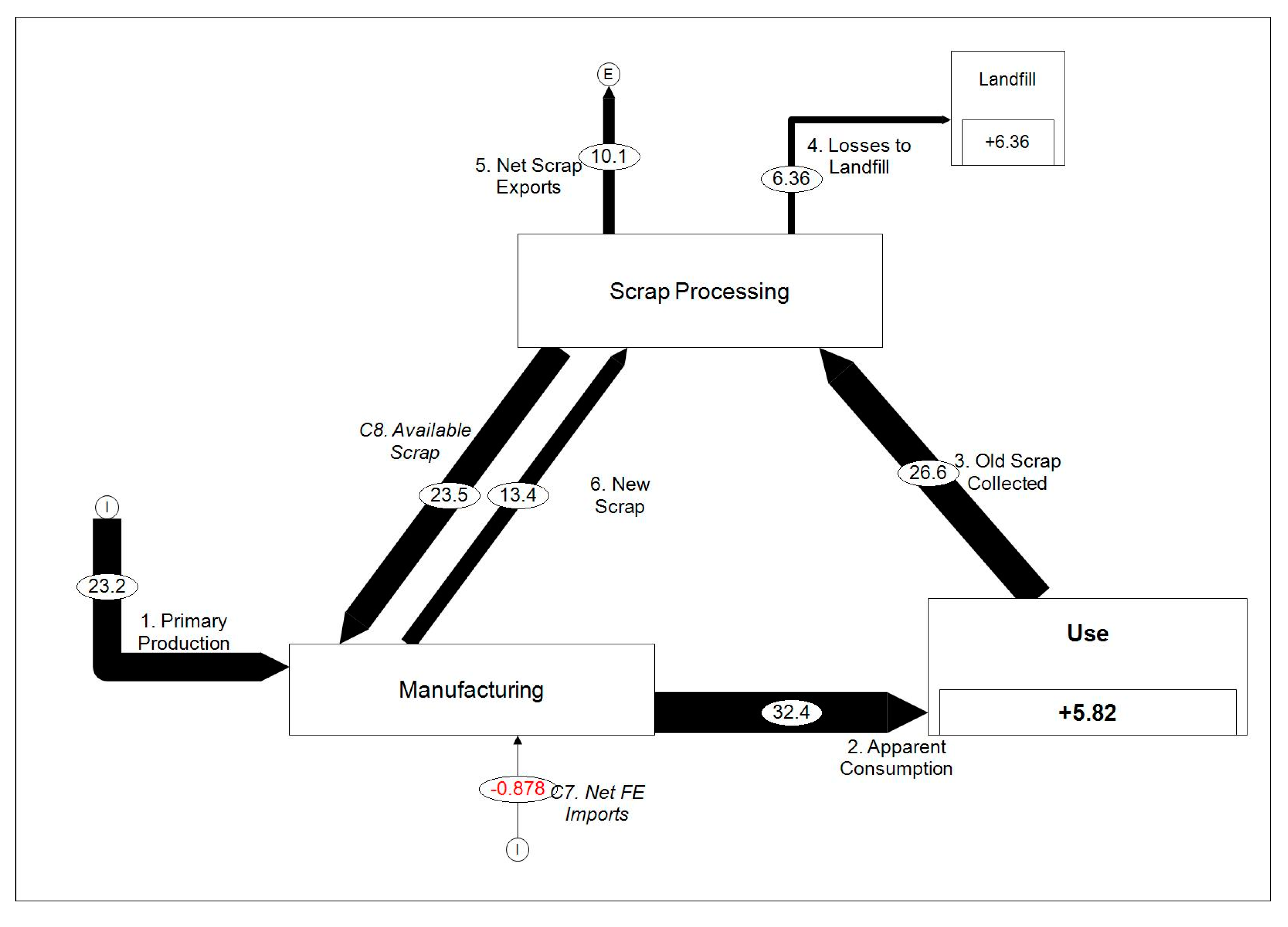
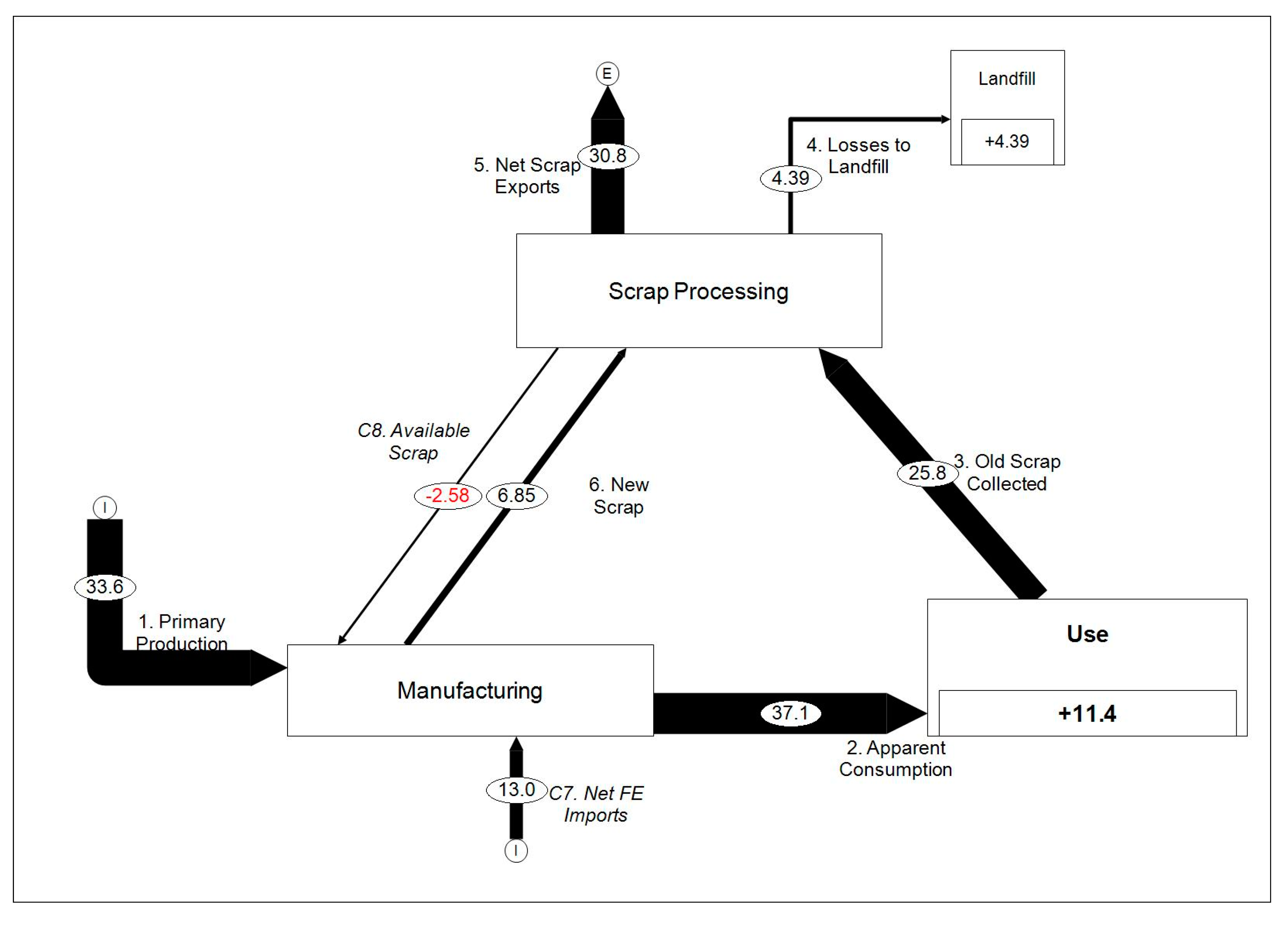
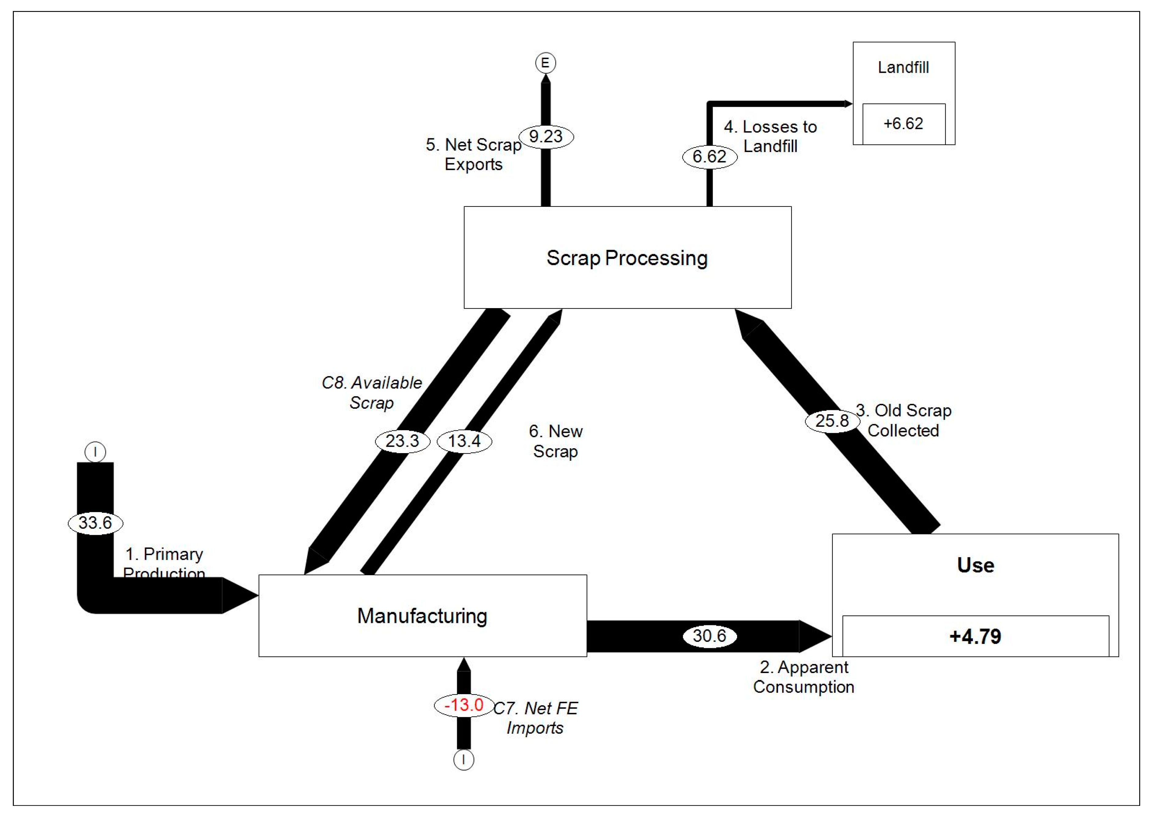
3.2. Scenario Analysis Results Scenarios (FS2–FS6)

Scenarios FS2 and FS3, as described in Table 2, were developed as bounding forecasts of changes in materials flows, and the results of these forecasts are presented in Figure 6, overlaid with FS1 results and observed historical data. Complete data series for these forecast scenarios are available in the Supplemental Information Tables SI-6 and SI-7. The bounding scenarios are based on fast rate-of-change and slow rate-of-change scenarios, in which the driver projections all accelerate beyond their current trajectory or slow significantly from it. These projections are then used with the expected case regression results (described in Equation (1) and Table 4) to estimate the bounding outcomes FS2 and FS3. These scenarios are considered less likely than FS1, but provide context into the maximum and minimum change for each flow. Scenario FS2, the slower driver change scenario, is shown in the life cycle framework in Figure 7. The result of a slowing in the drivers is a generally more circular scenario, with a smaller use-phase stock accumulation, more new scrap recovery, and less primary production, and even a complete reduction in necessary front-end imports to zero, with an excess of primary materials available, and therefore the U.S. transitioning to be again a net exporter of materials. Total consumption and landfilling rates, however, increase from the base case. Scenario FS3, the faster driver change scenario, shown in Figure 8, has very different results. Apparent consumption and primary production increase dramatically from the base case, without a corresponding increase in collection, leading to a significantly larger in-use stock accumulation. Scrap exports, additionally, increase about 50% from the base case, which, combined with the decrease in new scrap recovery results in a deficit of scrap availability. This net negative available scrap, means that there would not be enough available scrap to subsidize manufacturing demand for secondary materials. These drastically different results are due to the different relationships between individual flows and drivers. As discussed in Section 3.1, some drivers are highly positively correlated with some flows, but negatively correlated with others, so a slowing of one, urbanization, for example, leads to increasing consumption and primary production, and decreasing end-of-life collection and landfilling. Additionally, the low rate-of-change and high rate-of-change projections also apply to all drivers, even ones with decreasing trends, or negative slopes, so where all drivers follow a high rate-of-change (as in FS3) the result is a fast increase in some drivers, such as population, as well as a fast decrease in others, such as manufacturing contribution to GDP.
While Scenarios FS2 and FS3 were developed as bounding forecasts, Scenarios FS4–6 were developed based on the findings from the regression modeling for the base case scenario FS1. One key finding from the FS1 modeling, as described in Section 3.1, were the relationships between population dynamics population and urbanization with the material flows. These findings lead to the hypothesis that a high-migration scenario, in which total population grows slowly, but urbanization grows quickly, may lead to a more circular system, with decreased primary production, apparent consumption, and scrap exports but increased end-of-life collection. This hypothesis is tested through the development of the population migration Scenario FS4. Other results from the economic variables in Scenario FS1 led to the development of Scenarios FS5 and FS6, the economic transition and economic stagnation scenarios. Consumption, the largest volume flow, and in many ways the most important driver of the copper life cycle overall because demand for materials is ultimately what needs to be met, is positively correlated with Mfg%. GDP is correlated with end-of-life activities collection and landfilling. This leads to the postulated economic transition Scenario FS5 in which GDP grows quickly to theoretically reduce landfilling, but the manufacturing industry contribution to GDP changes slowly, and may therefore decrease consumption. The inverse of this, an economic stagnation scenario, was developed in which GDP grows slowly and Mfg% changes (declines) quickly, to identify which correlation, negative or positive, is stronger.
Resultant forecasts for Scenario FS4, the population migration scenario, are shown graphically in the life cycle framework in Figure 9, and the complete data series are available in the Supplemental Information Table SI-7. Net scrap exports decreased over 56% from the base case, though landfilled scrap increased 35%. This, combined with a decrease in apparent consumption, results in a large quantity of available scrap, such that over 70% of demand could be met by recycled materials, and the U.S. actually becomes a net exporter of refined copper.
The economic scenarios, FS5 and FS6, shown in Figure 10 and Figure 11 respectively, show less overall change to the copper life cycle than the population migration Scenario FS4. Complete data series for these forecasts are available in the Supplemental Information SI-8 and SI-9. Both economic transition and economic stagnation do not result in a net cumulative change in quantity for any flow greater than 5.5%, indicating that population dynamics are a more critical driver of trends in copper flows than economic drivers alone.

3.3. Circularity Metrics for Evaulation of Scenario Analysis Results

Several dozen circular economy or circularity metrics exist that represent various aspects of the circular economy, including resource-efficiency, stocks and flows dynamics, and product-centric measures [34] Many of these metrics are applicable only to specific processes or products, not complete materials economies with diverse uses. However, a few metrics can be used to quantify the circularity of the scenarios for the copper lifecycle, and were calculated for all future scenarios, based on the results of each forecast scenario (FS1–6). Circularity metric results are shown in Table 5. The first circular economy metric included is consumption from recycled material, which is the amount of apparent consumption that is met from the available scrap flow. The second is waste production, or total material to landfill, and the third is import reliance, which shows the percent of total apparent consumption that comes from imported materials, not domestically produced primary copper or scrap.
Scenario FS4, population migration, has the best circularity profile. Consumption from scrap is the highest by a significant margin, and import reliance is the lowest. This scenario results in the U.S producing more copper than necessary to meet demand. FS3 has lower landfilling rates, but would not be considered the most circular since it has a fairly high import reliance, and there is a negative scrap availability. This outcome confirms the previous findings that population dynamics are the most powerful drivers when it comes to circularity.

3.4. Environmental Sustainabiltiy Implications and Estimated Footprint

Circularity, a holistic look of resource efficiency in the context of the life cycle of a mineral, is a key aspect of the environmental sustainability of mineral resources, but not the only one. Environmental sustainability of mining and mined resources has been a topic of study since the 1990s, and several metrics exist to evaluate environmental footprint [35]. Though there are dozens of potential indicators of environmental sustainability of mined materials, a few key metrics can be selected to provide insight. We considered fresh water consumption, solid waste production, PM (particulate matter) production, and carbon footprint to evaluate beyond volume of material the associated environmental impact of copper in the future.
Chen et al. performed a comparative life cycle assessment of primary and secondary copper production and identified the inputs and outputs necessary for 1000 kg of copper production [36]. Fresh water demand was identified as 29,600 kg for primary copper production, and only 1400 kg for secondary copper production. Solid waste production was identified as 106,000 kg per 1000 kg primary copper, and 1330 kg for the same amount of secondary copper. Primary copper production resulted in 10.5 kg of PM release where secondary copper production resulted in 2.62. This study identified CO2 output as well, but the carbon footprint estimates used for this analysis were identified from Nilsson et al. in a study specifically identifying carbon footprint of copper production, not just CO2 emissions, which also looked at more operations overall, thus providing a slightly better metric [37]. They identified the carbon footprint of primary copper production in the U.S. as 4000 kg per 1000 kg Cu, and the average secondary copper production carbon footprint as 1050 kg CO2,eq. Because the total amount of primary and secondary copper has been forecast in Scenarios FS1 and FS2, these values can be used to calculate the approximate impact of each scenario. The summarized results are provided in Table 6. The impacts associated in the forecast period 2015–2030 were calculated as well as the impacts observed in the period 2000–2015 for reference. The percent change for each future scenario from the historical data are provided in Table 7.
These results show that Scenario FS2, slower driver change, exhibited the most significant increase over the historical baseline for PM and carbon footprint, and that Scenario FS3, faster driver change, had the largest footprint for water consumption and solid waste production. FS6, economic stagnation, had the smallest environmental footprint in all categories, smaller even than Scenario FS4, population migration, which exhibited the best circularity profile. This juxtaposition indicates how important it is, when considering sustainability, to assess multiple metrics, not to consider only circularity, and not only the impact through footprint. Additionally, this analysis shows that in a base case scenario, FS1, the environmental footprint of copper production is predicted to increase significantly over what it has been for 1970–2015. Though the footprint of one ton of copper may potentially decline through technological advances or process efficiency improvements, it is unlikely that a 50% decrease in measured impacts would occur before 2030, emphasizing the importance of decreasing overall consumption to have a significant impact on improving sustainability.

4. Discussion and Conclusions

This study has developed six future scenarios for the complete life cycle of copper flows in the U.S. A base case scenario, FS1, was developed based on the quantitative assessment of existing relationships between seven drivers of material flows and six major material flows. Projections of the drivers then allowed for the independent forecasting of these six material flows, and the use of mass balance formulae allowed for the forecasting of two calculated flows and in-use stocks. This scenario is the expected outcome if driver trends continue along their current paths, and therefore may be considered the most accurate prediction of the future copper life cycle in the absence of any of the changes in trends that were used to develop FS2–6, which would be contingent, in reality, upon externalities such as social changes or new policy adoptions. The fresh water use and solid waste footprints of the base case scenario FS1 are about 50% higher than the those of historical production for the past 15 years, and PM production and carbon footprint are both about 40% higher. These measures indicate clearly that the environmental impact associated with copper production in the U.S. will continue to increase, even as consumption slows.
The additional scenarios were developed by considering variability in the projections of the drivers. Faster driver change and slower driver change projections were identified for five of the seven drivers. These were used under varying assumptions to develop five additional future scenarios in a scenario analysis.
Scenarios FS2 and FS3, slower and faster driver change, provided bounding scenarios for the base case considering likely maximum and minimum changes in trends. Results from the Scenario FS2 forecasts showed that when all the drivers slow from their current trajectory, primary production decreases from the base case, but consumption and end-of-life collection increase, decreasing import reliance. Results from Scenario FS3, when the rates of change for all drivers are accelerated, show that though production, consumption, and collection all increase, circularity of copper is not improved due to a large increase in scrap exports, and increased import reliance.
Scenarios FS4, FS5, and FS6 were developed based on results from the relationships identified for Scenario FS1 to identify opportunities for improving the overall circularity of copper. Scenario FS4 is representative of a U.S. future in which the rate of population growth slows and people live in denser and therefore more resource-efficient societies. This theoretical future resulted in the most improvement for copper circularity, with total consumption, import reliance, scrap exports and landfilling decreasing, and available scrap for recycling and reuse increasing significantly beyond the base case scenario. Scenarios FS5 and FS6 were developed to explore potential economic transitions, in which only GDP and Mfg% were varied, and all other drivers followed base case trends. Both of these scenarios did not result in significant changes from the base case Scenario FS1.
A key finding of this study was that factors related to population changes impact significantly the entire life cycle of copper, suggesting that policy changes to incentivize urbanization increases without increasing overall population may be the most effective approach to increasing the circularity of copper in the U.S. Another finding was that an increase in collection of end-of-life scrap does not necessarily lead to an increase in scrap available for reuse in the U.S., due to the linked nature of end-of-life activities. This result is important in considering technological or policy changes that may possibly unlink these flows from their dependence on collection.
Finally, results indicated the importance, when considering sustainability, of assessing both the circularity as well as standard environmental impact metrics. Whereas Scenario FS4 yielded results with the highest level of copper circularity, Scenario FS6 yielded the smallest environmental footprint metrics, indicating a need to improve copper environmental footprint per unit. Improved efficiency of processing copper would reduce the environmental footprint per unit, whereas increased circularity will reduce the overall demand for primary materials.

Supplementary Materials

The following are available online at https://www.mdpi.com/2071-1050/11/20/5624/s1, Table SI-1: Historical Material Flow Driver Data and Sources, 1970-2015, Table SI-2: Historical Copper Life Cycle Material Flow Data, 1970-2015 (tons), Table SI-3: Projected Material Flow Driver Data Ranges and Sources (2016-2030), Figure SI-1: Q-Q Plots - Logistically Transformed Material Flow Drivers and their Respective Inverse CDFs, Table SI-4: Logistically Transformed Material Flow Driver Correlation Coefficients. The threshold for rejection is α = 0.1, or correlation coefficients < 0.9, Table SI-5: Scenario FS1 Forecasts of Copper Flows (Values are in Thousand Metric Tons/Year), Table SI-6: Scenario FS2 Forecasts of Material Flows (Values are in Thousand Metric Tons/Year), Table SI-7: Scenario FS3 Forecasts of Material Flows (Values are in Thousand Metric Tons/Year), Table SI-8: Scenario FS4 Forecasts of Material Flows (Values are in Thousand Metric Tons/Year), Table SI-9: Scenario FS5 Forecasts of Material Flows (Values are in Thousand Metric Tons/Year), Table SI-10: Scenario FS6 Forecasts of Material Flows (Values are in Thousand Metric Tons/Year).

Author Contributions

Conceptualization, M.R.G. and D.A.D.; methodology, M.R.G. and D.A.D.; validation, M.R.G. and D.A.D.; formal analysis, M.R.G..; investigation, M.R.G.; resources, M.R.G..; data curation, M.R.G.; writing—original draft preparation, M.R.G.; writing—review and editing, D.A.D.; visualization, M.R.G..; supervision, D.A.D.; funding acquisition, M.R.G. and D.A.D.

Funding

This work was supported by a Steinbrenner Institute U.S. Environmental Sustainability Ph.D. Fellowship to Miranda Gorman. The fellowship program was supported by a grant from the Colcom Foundation and by the Steinbrenner Institute for Environmental Education and Research at Carnegie Mellon University. Additional support for the study was provided by a College of Engineering Dean’s Fellowship to Miranda Gorman, and by the Hamerschlag University Professorship of David Dzombak.

Conflicts of Interest

The authors declare no conflict of interest.

References

  1. Gorman, M.R.; Dzombak, D.A. Stocks and Flows of Copper in the U.S.: Analysis of Circularity 1970–2015 and Potential for Increased Recovery. Resour. Conserv. Recycl. in press.
  2. Fishman, T.; Schandl, H.; Tanikawa, H.; Walker, P.; Krausmann, F. Accounting for the Material Stock of Nations. J. Ind. Ecol. 2014, 18, 407–420. [Google Scholar] [CrossRef] [PubMed] [Green Version]
  3. Schandl, H.; Hatfield-Dodds, S.; Wiedmann, T.; Geschke, A.; Cai, Y.; West, J.; Newth, D.; Baynes, T.; Lenzen, M.; Owen, A. Decoupling Global Environmental Pressure and Economic Growth: Scenarios for Energy Use, Materials Use and Carbon Emissions. J. Clean. Prod. 2016, 132, 45–56. [Google Scholar] [CrossRef]
  4. Gordon, R.B.; Bertram, M.; Graedel, T.E. Metal Stocks and Sustainability. Proc. Natl. Acad. Sci. USA 2006, 103, 1209–1214. [Google Scholar] [CrossRef]
  5. Zeltner, C.; Bader, H.-P.; Scheidegger, R.; Baccini, P. Sustainable Metal Management Exemplified by Copper in the USA. Reg. Environ. Chang. 1999, 1, 31–46. [Google Scholar] [CrossRef]
  6. Gerst, M.D. Linking Material Flow Analysis and Resource Policy via Future Scenarios of In-Use Stock: An Example for Copper. Environ. Sci. Technol. 2009. [Google Scholar] [CrossRef]
  7. Elshkaki, A.; Graedel, T.E.; Ciacci, L.; Reck, B. Copper Demand, Supply, and Associated Energy Use to 2050. Glob. Environ. Chang. 2016, 39, 305–315. [Google Scholar] [CrossRef]
  8. Meinert, L.; Robinson, G.; Nassar, N. Mineral Resources: Reserves, Peak Production and the Future. Resources 2016, 5, 14. [Google Scholar] [CrossRef]
  9. Labys, W.C.; Waddell, L.M. Commodity Lifecycles in US Materials Demand. Resour. Policy 1989, 15, 238–252. [Google Scholar] [CrossRef]
  10. Wernick, I.K.; Herman, R.; Govind, S.; Ausubel, J.H. Materialization and Dematerialization: Measures and Trends. Daedalus Natl. Acad. Tecbahia 1996, 125. Available online: https://phe.rockefeller.edu/Daedalus/Demat/ (accessed on 11 October 2019).
  11. Steinberger, J.K.; Krausmann, F.; Eisenmenger, N. Global Patterns of Materials Use: A Socioeconomic and Geophysical Analysis. Ecol. Econ. 2010, 69, 1148–1158. [Google Scholar] [CrossRef]
  12. Steger, S.; Bleischwitz, R. Drivers for the Use of Materials across Countries. J. Clean. Prod. 2011, 19, 816–826. [Google Scholar] [CrossRef]
  13. U.S. Geological Survey. Copper statistics [through 2015; last modified 2017]. In Historical Statistics for Mineral and Material Commodities in the United States U.S. Geological Survey Data Series; Kelly, T.D., Matos, G.R., Eds.; U.S. Geological Survey: Reston, VA, USA, 2017; Volume 140, p. 4. Available online: https://www.usgs.gov/centers/nmic/historical-statistics-mineral-and-material-commodities-united-states (accessed on 11 October 2019).
  14. Zhang, C.; Chen, W.-Q.; Ruth, M. Measuring Material Efficiency: A Review of the Historical Evolution of Indicators, Methodologies and Findings. Resour. Conserv. Recycl. 2018, 132, 79–92. [Google Scholar] [CrossRef]
  15. Gorman, M. US Copper Life Cycle Data. Kilthub Data Repos. 2019. [Google Scholar] [CrossRef]
  16. Bretschger, L. Energy Prices, Growth, and the Channels in between: Theory and Evidence. Resour. Energy Econ. 2015, 39, 29–52. [Google Scholar] [CrossRef]
  17. Liu, R.Q.; Jacobi, C.; Hoffmann, P.; Stober, G.; Merzlyakov, E.G. A Piecewise Linear Model for Detecting Climatic Trends and Their Structural Changes with Application to Mesosphere/Lower Thermosphere Winds over Collm, Germany. J. Geophys. Res. Atmos. 2010, 115. [Google Scholar] [CrossRef]
  18. Campra, P.; Morales, M. Trend analysis by a piecewise linear regression model applied to surface air temperatures in Southeastern Spain (1973–2014). Nonlinear Process. Geophys. 2016. Available online: http://doi.org/10.5194/npg-2016-29 (accessed on 11 October 2019).
  19. U.S. Census Bureau. Section 1. Population. Statistical Abstract of the United States: 2012. Available online: https://www.census.gov/library/publications/2011/compendia/statab/131ed/population.html (accessed on 11 October 2019).
  20. U.S. Census Bureau. 2017 National Population Projections Datasets. 2017. Available online: https://www.census.gov/data/datasets/2017/demo/popproj/2017-popproj.html (accessed on 11 October 2019).
  21. UN Population Division. World Urbanization Prospects: The 2018 Revision. 2018. Available online: https://esa.un.org/unpd/wup/Download/Files/WUP2018-F02-Proportion_Urban.xls (accessed on 11 October 2019).
  22. U.S. Geological Survey. Metal prices in the United States through 2010: U.S. Geological Survey Scientific Investigations Report 2012–5188. 2013; p. 204. Available online: http://pubs.usgs.gov/sir/2012/5188 (accessed on 11 October 2019).
  23. World Bank Commodity Markets. World Bank Commodities Price Forecast [April 2019]. 2019. Available online: http://pubdocs.worldbank.org/en/598821555973008624/CMO-April-2019-Forecasts.pdf (accessed on 11 October 2019).
  24. World Bank. GDP, United States. 2017. Available online: https://data.worldbank.org/indicator/NY.GDP.MKTP.CD?locations=US (accessed on 11 October 2019).
  25. U.S. Department of Agriculture. Real GDP (2010 dollars) Projection, International Macroeconomic Data Set. Economic Research Service. 2018. Available online: https://www.ers.usda.gov/data-products/international-macroeconomic-data-set.aspx (accessed on 11 October 2019).
  26. World Bank Data Bank. World Development Indicators. 2019. Available online: https://databank.worldbank.org/reports.aspx?source=2&series=NY.GDP.MKTP.CD,NV.AGR.TOTL.ZS,NV.IND.TOTL.ZS,NV.IND.MANF.ZS,NV.SRV.TOTL.ZS (accessed on 11 October 2019).
  27. UN Statistics Division. Indicator 12.2.2, Domestic Materials Consumption. UN Sustainable Development Goal Indicators. 2019. Available online: https://unstats.un.org/sdgs/indicators/database/ (accessed on 11 October 2019).
  28. Lorenz, M.O. Methods of measuring the concentration of wealth. J. Am. Stat. Assoc. 1905, 70, 209–219. [Google Scholar] [CrossRef]
  29. Wasserman, G.S.; Vijit, P.J. Use of Q-Q plots for comparing life data. Quality Congress. ASQ’s Annu. Qual. Congr. Proc. 2003, 57, 183–194. Available online: https://search-proquest-com.proxy.library.cmu.edu/docview/214386221?accountid=9902 (accessed on 11 October 2019).
  30. OECD. Real GDP Long-Term Forecast. 2019. Available online: https://data.oecd.org/gdp/real-gdp-long-term-forecast.htm#indicator-chart (accessed on 11 October 2019).
  31. UN Population Division. World Population Prospects 2019. 2019. Available online: https://population.un.org/wpp/Download/Standard/Population/ (accessed on 11 October 2019).
  32. Krausmann, F.; Gingrich, S.; Eisenmenger, N.; Erb, K.H.; Haberl, H.; Fischer-Kowalski, M. Growth in Global Materials Use, GDP and Population during the 20th Century. Ecol. Econ. 2009, 68, 2696–2705. [Google Scholar] [CrossRef]
  33. Reuter, M. (UNEP). Metal Recycling: Opportunities, Limits, Infrastructure; UNEP: Nairobi, Kenya, 2013. [Google Scholar]
  34. Parchomenko, A.; Nelen, D.; Gillabel, J.; Rechberger, H. Measuring the Circular Economy—A Multiple Correspondence Analysis of 63 Metrics. J. Clean. Prod. 2019, 210, 200–216. [Google Scholar] [CrossRef]
  35. Gorman, M.R.; Dzombak, D.A. A Review of Sustainable Mining and Resource Management: Transitioning from the Life Cycle of the Mine to the Life Cycle of the Mineral. Resour. Conserv. Recycl. 2018, 137. [Google Scholar] [CrossRef]
  36. Chen, J.; Wang, Z.; Wu, Y.; Li, L.; Li, B.; Pan, D.; Zuo, T. Environmental Benefits of Secondary Copper from Primary Copper Based on Life Cycle Assessment in China. Resour. Conserv. Recycl. 2019, 146, 35–44. [Google Scholar] [CrossRef]
  37. Ekman Nilsson, A.; Macias Aragonés, M.; Arroyo Torralvo, F.; Dunon, V.; Angel, H.; Komnitsas, K.; Willquist, K. A Review of the Carbon Footprint of Cu and Zn Production from Primary and Secondary Sources. Minerals 2017, 7, 168. [Google Scholar] [CrossRef]
Figure 1. Major flows of copper in the U.S. 1970–2015, Data from Gorman, 2019 [15], and available in Table SI-2.
Sustainability 11 05624 g001
Figure 2. Linearity in primary data for drivers Manufacturing contribution to GDP (Mfg%) and Domestic Materials Consumption (DMC).
Sustainability 11 05624 g002
Figure 3. The U.S. copper circular economy: major life cycle flows. Flows 1–6 are forecast using a regression model and driver projections, and C7 and C8 are calculated flows based on stocks and flows mass balance formulae.
Sustainability 11 05624 g003
Figure 4. Materials flow forecasts for Future Scenario (FS) 1 from regression analyses shown for years 2000–2030 with observed data. EoL, end-of-life
Sustainability 11 05624 g004
Figure 5. Cumulative copper life cycle forecast for Scenario FS1 for 2015–2030 in million metric tons.
Sustainability 11 05624 g005
Figure 6. Copper flow forecasts for Scenarios FS1, FS2, and FS3 for 2015–2030 in thousand metric tons shown with observed historical data. FS1 is represented by the solid line, FS2 is the dashed line, and FS3 is the dotted line. Observed data are represented by circles.
Sustainability 11 05624 g006
Figure 7. Cumulative copper life cycle flows for the slower driver change Scenario FS2 forecast for 2015−2030 in million metric tons.
Sustainability 11 05624 g007
Figure 8. Cumulative copper life cycle flows for the faster driver change Scenario FS3 forecast for 2015−2030 in million metric tons.
Sustainability 11 05624 g008
Figure 9. Cumulative copper life cycle flows for the population migration Scenario FS4 forecast for 2015−2030 in million metric tons.
Sustainability 11 05624 g009
Figure 10. Cumulative copper life cycle flows for the economic transition Scenario FS5 forecast for 2015–2030 in million metric tons.
Sustainability 11 05624 g010
Figure 11. Cumulative copper life cycle flows for the economic stagnation Scenario FS6 forecast for 2015–2030 in million metric tons.
Sustainability 11 05624 g011
Table 1. Material flow drivers, units, and sources for data series used for regression analysis.
Material Flow DriverUnitSource for Historical Data 1970–2015 or Most Recently AvailableSource for Expected Projection 2015–2030
TimeYear 1970–2030
Population106 PeopleU.S. Census Bureau, 2012 [19]U.S. Census Bureau, 2017 [20]
Urbanization% of popUN Population Division, 2018 [21]UN Population Division, 2018 [21]
Copper PriceCents/lbUSGS, 2013 [22]; USGS, 2017 [13]World Bank Commodity Markets, 2019 [23]
GDP109 US 2010 $World Bank, 2017 [24]USDA, 2018 [25]
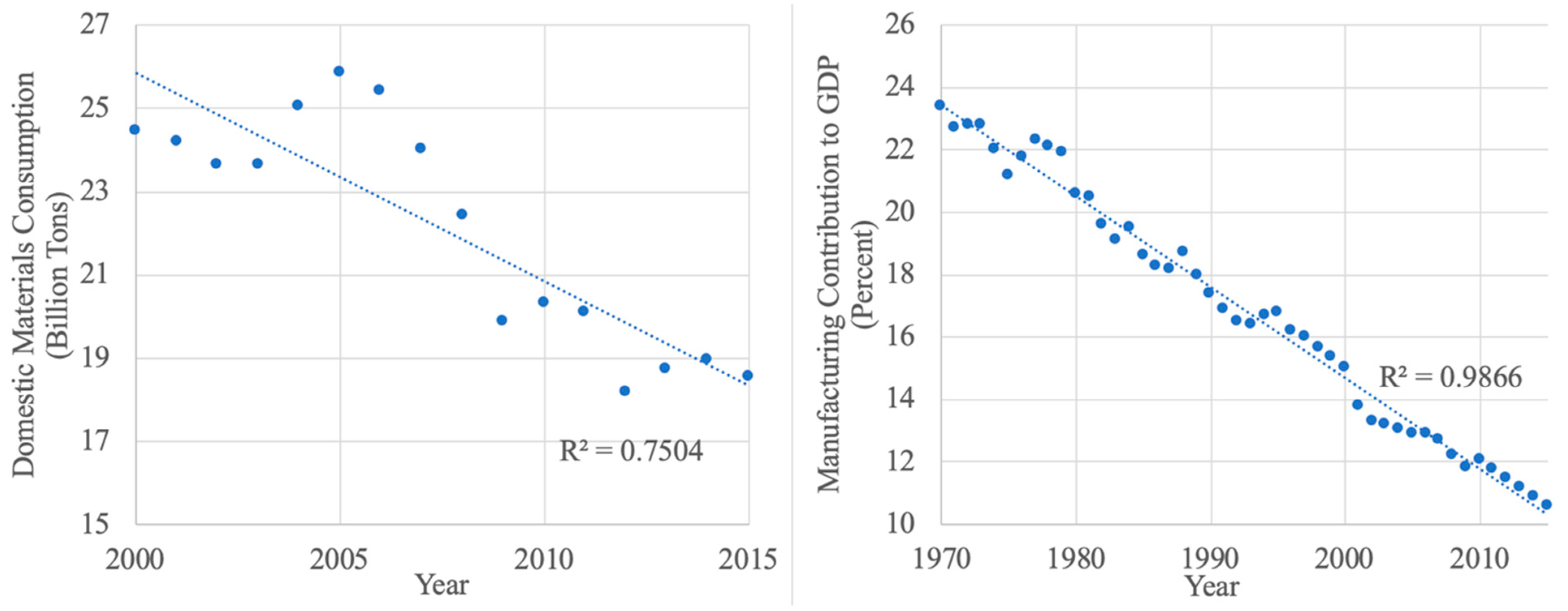
Manufacturing Contribution to GPD (Mfg%)% GDPWorld Bank DataBank, 2019 [26]Linearly Projected *
Domestic Materials Consumption (DMC)106 tonnesUN Statistics Division, 2019 [27]Linearly Projected *
* The linear trends that were used for the basis of these projections are shown in Figure 2.
Table 2. Future scenarios (to 2030) for the copper life cycle material flows, and the driver projections used in all six future scenario forecasts (sources in Table 3).
Forecast ScenarioDescriptionPopulation Increase RateGDP Increase RateMfg% Decrease RateDMC Decrease RateUrbanization Increase RateCopper Price
FS1Base CaseExpected outcome based on expected driver projectionsExpectedExpectedExpectedExpectedExpectedExpected
FS2Slower driver changeOutcome if drivers change more slowly than expected *LowLowLowLowLowExpected
FS3Faster driver changeOutcome if drivers change more quickly than expected *HighHighHighHighHighExpected
FS4Population MigrationSlower population increase; faster urbanization increaseLowExpectedExpectedExpectedHighExpected
FS5Economic transitionFaster GDP growth, slower decline in Mfg%ExpectedHighLowExpectedExpectedExpected
FS6Economic stagnationSlower GDP growth, faster decline in Mfg%ExpectedLowHighExpectedExpectedExpected
* Note that some drivers are increasing, where others are decreasing, so “change” refers to the rate of change, positive or negative: “slower” change indicates a smaller absolute value of the slope of the driver change with time, where “faster” change is a larger absolute value slope.
Table 3. Sources for driver projections used in forecasts. OECD, Organization for Economic Co-operation and Development
DriverLow Rate-of-Change ProjectionExpected ProjectionHigh Rate-of-Change Projection
PopulationZero migration scenarioU.S. Census Bureau, 2017 [20]High variant scenario
UN Population Division, 2019 [31]UN Population Division. 2019 [31]
Urbanization95% confidence interval linear fitUN Population Division, 2018 [21]95% confidence interval of linear fit
Copper PriceExpected projection was used in all scenarios
World Bank Commodity Markets, 2019 [23]
GDPOECD 2019 [30]Expected projection used also for high rate-of-change USDA, 2018 [25]
Mfg%95% confidence interval of initial linear regressionLinear Projection95% confidence interval of initial linear regression
DMC95% confidence interval of initial linear regressionLinear Projection95% confidence interval of initial linear regression
Table 4. Regression results, α and β coefficients (with p-values in italics) relating drivers to material flows and R2 values associated with the resulting equations.
Material Flows (Fj)
1. Primary Production2. Consumption3. EoL Collection4. Landfilled Scrap5. Scrap Exports6. New Scrap
Intercept (α)67305155−1333−1896202−1486
β values for Drivers (p-values)Year−1010
(2 × 10⁻³)
−806
(2 × 10⁻²)
180
(5 × 10⁻⁸)
28
(2 × 10⁻⁵)
210 (1 × 10⁻³)
Urbanization221
(4 × 10⁻³)
223
(6 × 10⁻³)
−84.9
(5 × 10⁻³)
Population −7.72
(8 × 10⁻³)
32.2
(2 × 10⁻³)
−17.6
(2 × 10⁻⁴)
Cu Price −0.239
(8 × 10⁻³)
0.21
(8 × 10⁻⁴)
0.136
(7 × 10⁻³)
0.169
(1 × 10⁻³)
GDP −2.17
(3 × 10⁻⁵)
−1.46
(7 × 10⁻³)
Mfg% 3.58
(7 × 10⁻⁴)
DMC 0.861
(9 × 10⁻³)
R20.800.950.990.980.950.94
Table 5. Measures of Circular Economy Metrics for Scenarios FS1–6, 2015–2030.
Circular Economy Metrics
ScenarioConsumption from Recycled Material (% of Demand Met by Available Scrap)Waste Production (Thousand Tons)Import Reliance (% of Demand from Imports)
FS125%492619%
FS272%6364Net exporter (0.9 Mt)
FS3N/A439135%
FS477%6221Net exporter (13 Mt)
FS524%503124%
FS630%4921125%
Table 6. Cumulative Environmental Footprint of Copper Production for 15 year time periods: 2015–2030 Forecast Scenarios FS1–FS6, and 2000–2015 Historical, Observed Data as a baseline.
Fresh Water (Million Tons)Solid Waste (Billion Tons)PM (Thousand Tons)Carbon Footprint (Billion Tons)
Future Scenarios:
FS1 9613.413581.37
FS29923.474021.54
FS311003.943901.49
FS49383.273831.47
FS510103.583751.43
FS69133.243431.31
Observed Scenario:
2000–20156452.262570.984
Table 7. Environmental Footprint Metrics Percent Change in 2015–2030 forecast from 2000–2015 Baseline.
ScenarioFresh WaterSolid WastePMCarbon Footprint
FS149%51%40%39%
FS254%53%57%57%
FS370%74%52%51%
FS445%45%49%49%
FS556%58%46%46%
FS642%43%34%33%

