Article

Assessing the Impact of Land Cover Changes on Surface Urban Heat Islands with High-Spatial-Resolution Imagery on a Local Scale: Workflow and Case Study

1
State Key Laboratory of Subtropical Building Science, Department of Architecture, South China University of Technology, Guangzhou 510640, China
2
Architectural Design Research Institute of SCUT, Guangzhou 510640, China
3
Institute of Geography and Tourism, Guangdong University of Finance & Economics, Guangzhou 510320, China
*
Author to whom correspondence should be addressed.
Sustainability 2019, 11(19), 5188; https://doi.org/10.3390/su11195188
Submission received: 23 July 2019 / Revised: 19 September 2019 / Accepted: 20 September 2019 / Published: 22 September 2019

Abstract

:
Low-altitude remote sensing platform has been increasingly applied to observing local thermal environments due to its obvious advantage in spatial resolution and apparent flexibility in data acquisition. However, there is a general lack of systematic analysis for land cover (LC) classification, surface urban heat island (SUHI), and their spatial and temporal change patterns. In this study, a workflow is presented to assess the LC’s impact on SUHI, based on the visible and thermal infrared images with high spatial resolution captured by an unmanned airship in the central area of the Sino-Singapore Guangzhou Knowledge City in 2012 and 2015. Then, the accuracy assessment of LC classification and land surface temperature (LST) retrieval are performed. Finally, the commonly-used indexes in the field of satellites are applied to analyzing the spatial and temporal changes in the SUHI pattern on a local scale. The results show that the supervised maximum likelihood algorithm can deliver satisfactory overall accuracy and Kappa coefficient for LC classification; the root mean square error of the retrieved LST can reach 1.87 °C. Moreover, the LST demonstrates greater consistency with land cover type (LCT) and more fluctuation within an LCT on a local scale than on an urban scale. The normalized LST classified by the mean and standard deviation (STD) is suitable for the high-spatial situation; however, the thermal field level and the corresponded STD multiple need to be judiciously selected. This study exhibits an effective pathway to assess SUHI pattern and its changes using high-spatial-resolution images on a local scale. It is also indicated that proper landscape composition, spatial configuration and materials on a local scale exert greater impacts on SUHI.

1. Introduction

Against the background of extensive urbanization, cities and conurbations experience rapid expansions, especially in developing countries. Vast areas of rural land are changed into impervious surfaces such as buildings and roads, which generally absorb and re-radiate solar radiations effectively [1,2,3,4,5]. These easily-stored solar radiations and artificial heat generated from productions, transportations, and civilian life lead to severe urban heat islands (UHI) [6,7,8,9]. This phenomenon, as a chief corollary of urbanization, critically affects not only the urban environment and ecology but also human health [10,11,12]. Consequently, how to mitigate these impact of the UHI effect has become one of the hot research issues since the inevitability of urbanization [13].
Research has been proliferating on the analysis of the patterns of UHIs, their influences, and corresponding adaptive strategies [14,15,16,17]. These studies are usually based on the relationship between land surface temperature (LST) and land cover (LC) [18,19,20], which play crucial roles in describing the urban thermal environment. The outcomes generally confirm that LST is negatively correlated with the abundance of vegetation while it is positively correlated with the percentage of impervious surfaces area [21,22]. Some studies also pay attention to the difference of regions, seasons, and even moments during a day. Tarawally et al. [23] compared the responses of LST to LC changes in the long term between the coastal and inland cities. According to Roth et al., for some American cities, the difference between urban and rural LSTs in the daytime was larger than that at night [24]. Furthermore, to reduce interference from other factors and assess SUHI quantitively, some researchers provided and examined evaluative indexes [25,26]. Pongracz et la. [27] found that the surface urban heat island intensity (SUHII) in nine central Europe cities demonstrated appreciable monthly variations.
Most of the researches on SUHI have been carried out by using thermal infrared (TIR) satellite remote sensing techniques. It is evident that the copious data accumulated from satellites over the decades suffice to enable the accurate determination of temporal and spatial change patterns of LC, LST and SUHI on both the macro- and meso-scales [28,29,30]. However, the scale and spatial resolution of imageries may occasionally determine the conclusions for studies. Luan et al. [31] analyzed the urban green land in Beijing with Landsat TM5 data with 120 m spatial resolution and showed that the patches’ perimeter, area, shape index, and fractional vegetation cover had no significant correlation with their cooling range on their surroundings; conversely, Gao et al. [32] obtained completely different conclusions by aerial photos with 0.25 m spatial resolution. Thanh Hoan et al. [25] regressed the multivariate relationship between land-use composition and LST, which had reasonable results at a specific window size only in the summer season. Thus, there is also a need to observe urban thermal environments with multi-scale remote sensing technologies [33,34].
Low-altitude airborne platforms as a complement to satellite-based remote sensing technologies are more suited for local or micro-scale studies [35,36,37]. The conventional method to collect TIR aerial data involves the use of manned airborne platforms, which can supply exceedingly high-quality imageries through the big thermal infrared multispectral scanner (with the requirement of a heavy load) [38,39,40,41,42]. However, logistical hindrances such as the costs of commissioned flights and limited technical resources circumscribe its wide application. Accordingly, a variety of unmanned airborne systems have in recent years been considered as an alternative due to their low costs and flexibility. Unmanned airborne systems with visible and TIR camera have hitherto been employed for various civil, industrial, and agricultural research and management [43,44,45], but rarely for research on local SUHI and its change patterns. This situation is partially due to technical restrictions such as the undesirably small observation areas of unmanned aerial vehicles (UAV), short flight duration (generally about 15–20 min) and overly low cruising altitudes (generally under 200 m) [46,47]; and also partially due to the lack of effective methods for common and inexpensive devices. Therefore, a reliable and affordable method is necessary to assess the SUHI on a local scale.
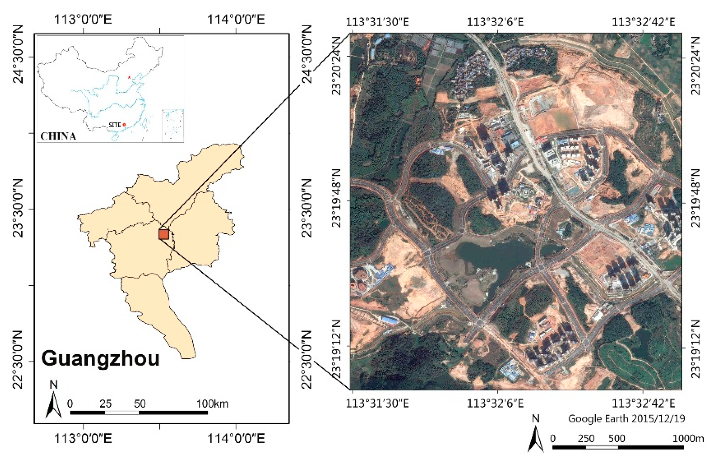
In this study, we first present a workflow to assess the LC’s impact on SUHI, based on the visible and TIR images with high spatial resolution captured by an unmanned airship system (UAS) [35] in the Sino-Singapore Guangzhou Knowledge City in 2012 and 2015. Moreover, we assess the accuracy of the LC classification and land surface temperature (LST) retrieval, and the applicability of some well-known indexes from satellite remote sensing field on a local scale, and finally analyze the spatial and temporal changes in the SUHI patterns.

2. Study Area and Data

2.1. Study Area

Guangzhou has a subtropical monsoon climate, with scorching weather and abundant rainfalls in the summer season. Monthly average temperatures reach up to 27.6 °C and 28.6 °C during June and August, respectively. The Sino-Singapore Guangzhou Knowledge City is located in the town of Jiulong, more than 30 km northeast away from the central city of Guangzhou. It planned to cover the land area of approximately 123 km2, and would poise as a culture-sharing city with global influences, independent innovation, and ecological livability. Its construction planning has been divided into three stages: a center area of around 10 km2 would mark the beginning of the project in 2010–2013; the construction would subsequently expand to about 30 km2 in the medium-term (2013–2020); and the entire construction of 50–60 km2 would be gradually completed in the long-term (after 2020). It is still developing rapidly now.
Our observation area, located in the southern start-up area, lies between approximately 23°19′00′′ to 23°20′30′′ latitude and 113°31′28′′ to 113°32′51′′ longitude, covering an area of 6.72 km2, as shown in Figure 1. Given its rapid conversion from a rural area into an urban one in a short time, our observation area is extremely suited for observing and analyzing the patterns of changes in LC, LST and SUHI.

2.2. Platform and Data Acquisition

In this study, an unmanned airship was used as a platform (Figure 2), which could lift a payload of up to 10 kg for a flight duration of up to 3 hours. It can automatically maintain the altitude and cruise according to a predefined route. The TIR imaging camera (TH9260) was responsible for taking TIR images that have one band with a spectral range of 8 to 13 μm. The digital SLR camera (Canon 450D with 18–55 mm F/3.5-5.6 IS) was used to obtain visible images. They were both mounted on a double three-axis platform. The favorably large payload and long duration enabled the simultaneous capture of visible and TIR images in one single flight. See Reference [35] for the integration of the whole system.
Outdoor data acquisition included the airborne observation and synchronous field measurement. The airship observing campaign at a height of 600 m was conducted between 12:00 and 12:30 on 23rd August 2012 and between 13:00 and 13:30 on 21st June 2015. The height is corresponding to the spatial resolution of visible and TIR images within 0.15 m and 0.8 m, respectively, as shown in Table 1. The airship observing method and principles were adopted from Reference [35].
To verify the accuracy of the LST retrieved, the typical surface temperatures were measured in synchrony with the airship observing campaign. In this field campaign, the contact temperature loggers (Ibutton and BES-1) with a circular planar contact sensor with an accuracy of 0.5 °C were used to measure the surface temperatures of trees, lawns, paddy water, water bodies, concrete pavements, asphalt pavements, building roofs, and soils at one-minute intervals.

3. Methodology

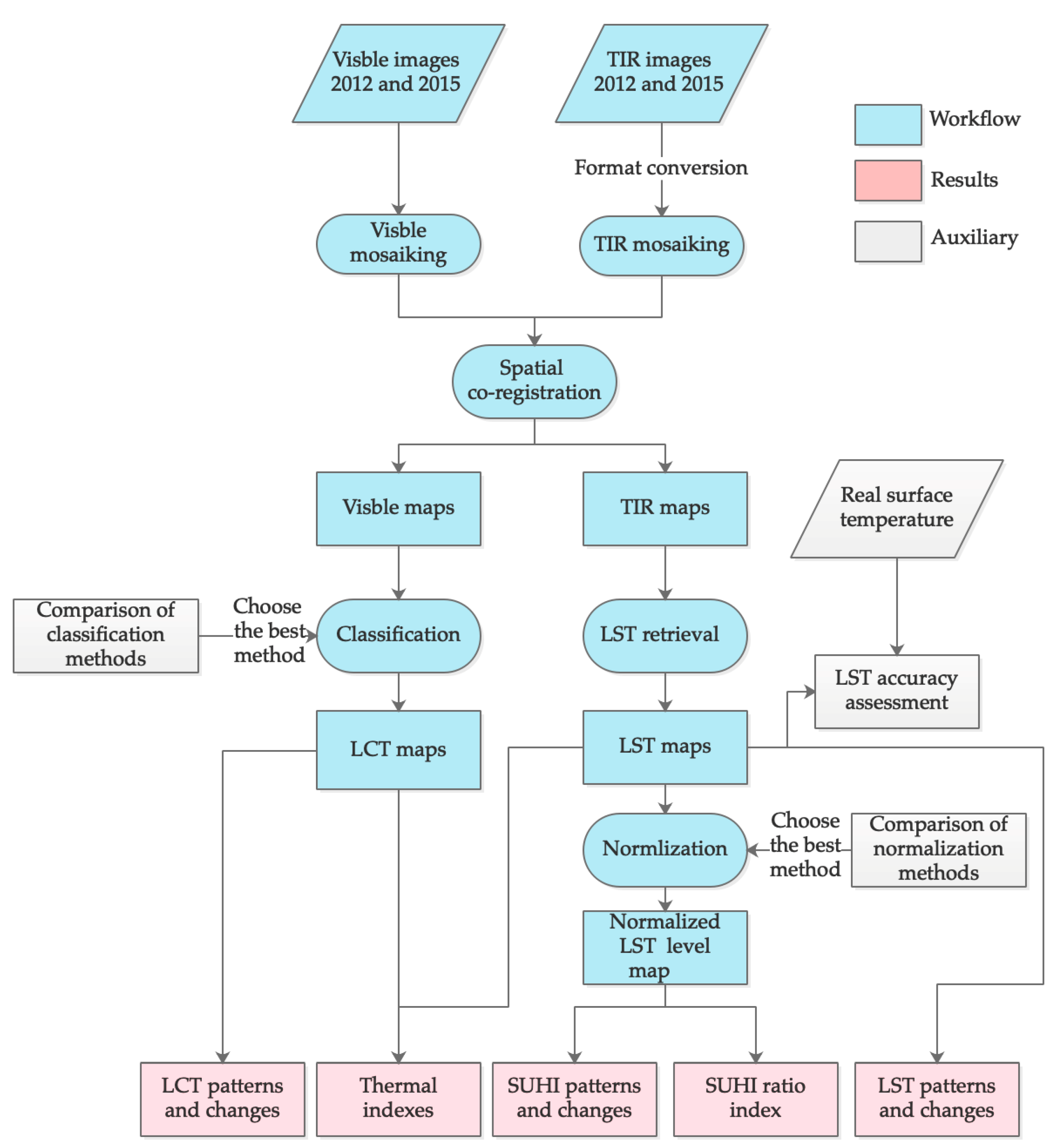
This study aims to determine the effective method to assess SUHI patterns based on LCTs and their changes on a local scale. The workflow is as follows (Figure 3). First, the visible and TIR images obtained by observations are mosaiced and orthorectified to visible and TIR orthophotos. Subsequently, the orthophotos are spatially co-registered to a high-resolution non-offset optical Google map. This is followed by the classification of the LCT from the visible map. Then, an LST map is retrieved from the TIR map based on the algorithm of TH9260. Finally, statistical analyses on LC, LST, and SUHI are performed. The following sections detail these phases and present the relevant data.

3.1. Pre-Processing

The hundreds of visible and TIR images need to be pre-processed, with regard to aspects including the mosaicking, geometric correction, and spatial co-registration. The mosaicking for both kinds of images was performed by the Agisoft PhotoScan software, which has been widely used in UAV image mosaicking [48]. For the visible orthomosaic, the processing with PhotoScan was twofold. Firstly, the software was deployed to identify and match the feature points between images with the Scale Invariant Feature Transform (SIFT) algorithm, and to reconstruct the scene geometry with Structure from Motion (SfM) techniques [49]. Then, it applied a dense multi-view reconstruction to the aligned images to establish the scene geometry, and finally exported an orthophoto [50]. The whole processing was automatic and involved no human interactions. The TIR images obtained from the TH9260 camera can be identified only by its companion software "Image Processor Pro II"; accordingly, the ASCII format file with the temperature information of each pixel had to be exported and converted into the Tiff format image through the IDL program in the ENVI software. For the TIR images, the subsequent mosaicking was performed in a manner similar that for the visible images [51].
The other pre-processing step is to perform spatial co-registration for the visible and TIR orthophotos, which is necessary for subsequent analyses on LCT and LST. We chose the non-offset optical Google map with geographic coordinates in the study area as the reference. The visible and TIR orthophotos in 2012 and 2015 were loaded into ArcMap and co-registered to the Google map with twenty as possible as evenly-distributed, clear, and discernible feature points e.g. intersections of roads and corners of houses in all maps. The second-order polynomial transformation was selected for this process in ArcMap.

3.2. Classification and Accuracy Assessment

Given the central role of the algorithm in ensuring successful classification, five supervised classification algorithms were deployed in the ENVI software [52]: Maximum likelihood, parallelepiped, minimum distance, Mahal distance, and neural network classification algorithms [53]. Based on land-use characteristics in the study area and spectral characteristics of the visible image, LC was identified and classified into six types: Dry farmland (including crops and lawns), paddy field, woodland, bare land, built-up land, and water body. After the classification, accuracy assessments were performed by comparing the consistency of validation data (over 500 checkpoints for each LCT) and the classification results for the different algorithms. Overall accuracy and kappa coefficient, as well as user’s accuracy and producer’s accuracy, were used as quantitively assessing indexes [54]. Finally, each LCT was extracted from the classified maps for discerning the changes in the areas during the period of interest in ArcMap.

3.3. LST Retrieval and Accuracy Assessment

Due to functional limitations of the TH9260, traditional satellite remote sensing methods cannot be directly applied. The LST retrieval has to be performed based on the corresponding function in the "Image Processor Pro II" software, which provides a retrieval algorithm based on the parametric correction of atmospheric transmittance, mean atmospheric temperature, and emissivity. This process is fourfold. First, we retrieved LST from the brightness temperature (BT) in the images (including a representative LCT) by correcting these aforesaid parameters. Next, we extracted the BT and LST of some corresponding sample pixels to regress their linear relationships. Then, we used the mask to extract the TIR maps for each LC according to the previous LC classification. Finally, we engaged spectral calculation to obtain the LST maps of each LCT based on the linear relationship between BT and LST, and then mosaicked them to the whole LST maps for 2012 and 2015.
The atmospheric correction was performed with the MODTRAN 4 model. In this paper, the settings of input parameters were in place [55]: the model atmosphere was selected as tropical; the atmospheric path was the slant path between two altitudes; the aerosol model was set to Rural Extinction; the default visibility was 5 km; the seasonal aerosol profile was set to Spring–Summer; the weather was fine, and no cloud or rain. The range of wavelengths was from 8 μm to 13 μm, and the wavelength space was set to 0.1 μm. The atmospheric temperature at the first boundary took the observed mean value during the airship’s campaign at flight altitudes (29 °C in 2012 and 28.5 °C in 2015). Assuming the spectral response functions on one broad spectral band of the TH9260 according to a normal distribution, the mean atmospheric transmittances were 0.64 in 2012 and 0.68 in 2015.
Given the lack of in situ measurement of the emissivity of LCTs and non-mixed pixels in our study, reference values released by the MODIS UCSB Emissivity Library were used to retrieve LST [56,57]. The mean values of emissivity (Table 2) are as follows: dry farmland (0.95), paddy field (0.97), woodland (0.96), barren land (0.96), built-up land (0.95), and water body (0.99). After LST retrieval, the surface temperatures recorded synchronously with the in-situ measurements were used to evaluate the accuracy of the retrieval results.

3.4. Thermal Indexes Based on LC

In this section, the thermal effect contribution index (Hi), thermal pixels proportion index (D1), and regional thermal pixels proportion index (D2) were used to discuss the impact of various LCTs on the urban thermal environment.
Hi indicates the impact on the regional mean LST caused by LCTs. For calculating Hi, we first aggregated the differences between the LSTs of the pixels on each LC higher than the regional mean LST as the initial thermal effect contribution index (Hi), and then normalized Hi to compare them among various LCTs. Hi and Hi are respectively calculated by Equation (1) and Equation (2),
H i = j = 1 n i ( T i j T a 0 )
H i = H i i = 1 n H i .
where Tij represents the LST of pixel j on the land cover i more than the regional mean LST, Ta0 the regional mean LST of the study area, ni the pixel numbers on the LCT i more than the regional mean LST. A greater Hi implies a more significant thermal effect of the LCT.
On the other hand, D1 and D2 are respectively represented by:
D 1 = n i N i
D 2 = n i N
where D1 represents the ratio of the area with LST above the mean in an LCT, D2 the ratio of the area with LST above the mean in the total study area, and Ni the pixel numbers on the LCT i, and N the total pixel numbers in the study area.

3.5. Normalized LST Level Map

Given differences in climate background, it will be challenging to directly compare LST maps across different years [58]. Accordingly, the normalized LST (NLST) could maintain the spatial distribution of LST and eliminate the influence of varied climate background, providing an objective comparison [59]. The LST maps need to be normalized by Equation (5) [60]:
L S T i = L S T i L S T m i n L S T m a x L S T m i n
where LSTi is the normalized LST of i pixel, LSTi the LST of i pixel, LSTmax and LSTmin respectively the maximum and minimum LST values in a map. Such normalization uniformly rescales the distribution of LST to the 0-and-1 range, as well as reduces the climatic differences.
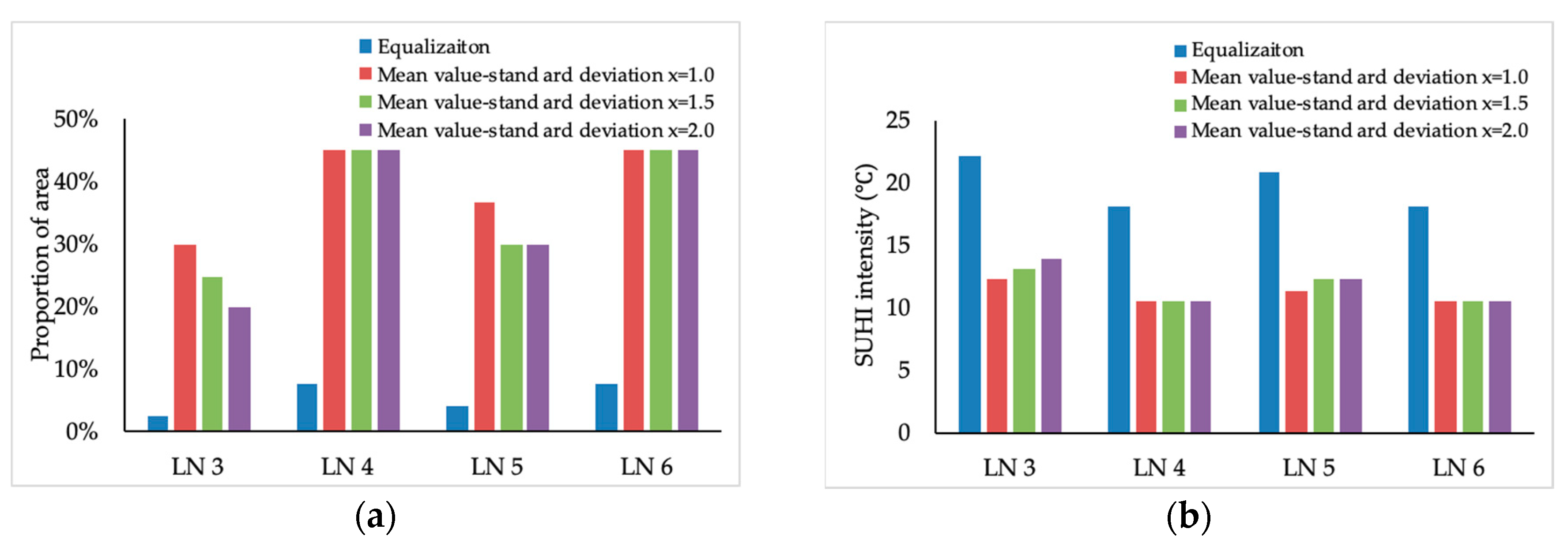
Then, we classified the NLST into different thermal field levels (from 3 to 6) through the equalization method and the mean value-standard deviation (STD) method (Table A3), and chose the preferred method and numbers of corresponding thermal field levels based on the results (Figure A1, Figure A2, Figure A3 and Figure A4) [61]. Subsequently, the area of each level and SUHI pattern were calculated and investigated during the period of interest. The primary purpose of the classification of the NLST was to understand the changes in the statistical distribution of temperature data and mitigate SUHI.

3.6. SUHI Ratio Index Computation

In order to further study SUHI variations between 2012 and 2015, the surface urban heat island ratio index (SUHIRI) is computed, as follows:
S U H I R I = 1 100 m i = 1 n W i P i
where m represents the level number in the previous normalized step, n the number of the levels higher than the mean temperature, Wi the weight of the levels higher than the mean temperature (the order value of the level in m, for example , the weight value of high and extra-high levels are 5 and 6, respectively), and Pi the area proportion of the SUHI level of i in the study area [59,61].

4. Results

4.1. Results of Mosiacking and of Spatial Co-registration

With the methods in Section 2.1, we obtain the co-registered visible and TIR mosaic maps in the study area for 2012 (Figure 4) and 2015 (Figure 5). For each mosaic map, objects such as various constructions and even their material characteristics are apparent and sharply-defined in the visible map, while the edges of the corresponding objects and their TIR distributions are obvious in the TIR map.
To assess co-registration accuracy, we checked the errors of some feature points between the Google map and the mosaic maps. The co-registration error and the root mean square error (RMSE) of each map are summarized in Table 3. The values of the RMSE for the visible maps were 0.74 pixel in 2012 and 0.80 pixel in 2015, while those for the TIR maps were correspondingly 2.33 pixels and 1.86 pixels. It is reasonable that the co-registration accuracy of the visible map with higher spatial resolution and more obvious object features was higher than that of the TIR map. The co-registration accuracy of both kinds of maps is regarded as satisfactory for LC classification and further analyses of the thermal environment.

4.2. LC Classification and Changes in Patterns

4.2.1. Assessment of LC Classification

We used the visible maps in 2012 and 2015 to assess the classification accuracy from different classification algorithms. From Table 4, it is evident that the maximum likelihood method has yielded the best result on the LC classification maps. For 2012 and 2015, the values for the overall accuracy were respectively 92.88% and 90.32%, while those for the Kappa coefficient were respectively 0.91 and 0.88 (Appendix A: Table A1 and Table A2 detail the classification results in 2012 and 2015 from the maximum likelihood method).

4.2.2. Patterns of LC Classification in 2012 and 2015

The results of the LC classification for 2012 and 2015 from the maximum likelihood algorithm are shown in Figure 6. It is readily discernible that areas of the built-up land and bare land have expanded rapidly from 2012 to 2015, at the expense of other LCT, especially woodland. Other observations are that the changes were mainly concentrated in the southwest and northeast areas, and that the changed areas were generally less than the unchanged ones.
The area proportion of each LCT was calculated, as shown in Table 5. From Figure 6 and Table 5, the order of the areas of the different LCTs did not change though the areas did vary drastically. The most dominant LCT was woodland, which also exhibited the most significant decline from 55.66% of the study area in 2012 to 35.49% in 2015. Built-up land and bare land were the two fastest-growing types, respectively expanding from 9.36% to 18.19% and from 17.87% to 29.60%, reflecting the robust and rapid development during these three years of analysis. Furthermore, the substantial growth of bare land earmarked for future constructions implies that the pace and extent of development would only continue and intensify in the future. For dry farmland and paddy field, their areas have witnessed only slight changes, thereby underlining the excellent protection bestowed upon agricultural land. Note that the increased proportion of dry farmland (3.58%) does not translate into the reclamation of new agricultural land. Two reasons underlie this, the first of which concerns the growth of lawns, which had hitherto not been classified separately due to their small total area and similar spectral properties in visible imageries. For example, the artificially-grown lawns near the Phoenix Lake (a large artificial lake) in 2015 were identified as dry farmland. The other reason concerns the variety of crop types and harvest. A little field without any crops but reflective water on the northwest side of the study area (Figure 6a) was classified as built-up land in August 2012; however, it was later re-classified as dry farmland with crops in June 2015. Additionally, the Phoenix Lake which appeared in 2015 did not lead to an increase in the area of the water body (from 4.84% to 3.05%) due to the disappearance of small-spread water bodies elsewhere.
To further characterize the temporal and spatial evolutions of LC in the study region, change detection analysis was used to determine the quantities of conversion from a particular LCT to another. A cross matrix (Table 6) provides information regarding the transition between LCTs. For the woodland, around 28.48% in 2012 was converted into bare land, 11.84% into built-up land, and 10.12% into dry farmland, illustrating that the major source of the developed and developing areas was founded on converted woodland. For the built-up land, around 21.20% was converted into bare land, meaning that existing constructions were demolished and that planning was underway for earmarking the land for new uses. Additionally, 14.61% and 13.61% of the built-up land were turned into dry farmland (most of them were lawns) and woodland respectively, thereby highlighting the importance of ecological protection during the development. For the bare land (representing the area that had been planned for construction in our case), it was converted into built-up land (24.3%), woodland (14.15%), and dry farmland (12.92%), suggesting a balance between urban development and ecological preservation.

4.3. LST Patterns and Changes

4.3.1. Assessment of LST Retrieval

The measured real surface temperature as reference points and the corresponding LST values for comparison are shown in Table 7. The temperature deviations between the retrieved and measured temperatures varied from –0.45 °C to 3.08 °C, and the mean of absolute deviation and RMSE were 1.63 °C and 1.87 °C, respectively. In general, water body, woodland, dry farmland, and paddy field have higher temperature accuracy than built-up land (building roof, asphalt pavements, and concrete pavement), given the relatively stable emissivity of the former four LCT and their temperature ranges that were similar to the ambient temperatures. The temperature deviations of built-up land ranged from 1.65 °C to 3.08 °C, mainly because the emissivity of the man-made impervious surfaces was set to be the same in this study. The broad emissivity of some pavement made by concrete may in fact vary from 0.85 to 0.96 in the database published by the MODIS UCSB Emissivity Library [56,57]. The temperature deviation of water in the Phoenix Lake was –0.45 °C, while the value of pool (small water body) was 1.63 °C, which is because of the much difference in their depth and volume.

4.3.2. LST Patterns and their Changes in 2012 and 2015

LST maps and their associated descriptive statistical results in 2012 and 2015 are shown in Figure 7 and Table 8, respectively. The results (Figure 7) reveal a generally increasing trend in the LST distributions from 2012 to 2015, as is consistent with the expansion of the built-up land in the study area (Figure 4 and Figure 5). The LST of the impervious areas such as the built-up land, especially roads, is noticeably higher than that of the pervious areas, such as the water body, woodland and so on, implying the impacts of construction activities of human being on the thermal environment.
From Table 8, the maximum LSTmean in 2012 was registered by the built-up land, followed by dry farmland, bare land, paddy field, water body, and finally by woodland, while the maximum LSTmean in 2015 was registered by the built-up land, followed by dry farmland, bare land, woodland, paddy field, and finally by water body. We noted that the LSTmean orders were the same for all LCTs except woodland, which exhibited the lowest LSTmean (26.99 °C) in 2012 but the third lowest one (36.69 °C) in 2015. The values of LSTmean on built-up land in 2012 and 2015 were both much higher than those of others because of its impervious characteristics such as thermal properties and anthropogenic activity [11,62]. Dry farmland with the second-highest LSTmean—which was even slightly higher than that of bare land and much higher than that of woodland—implied that dry farmland with low coverage did not contribute to cooling despite its vegetation. The values of LSTmean of woodland in 2012 and of water body in 2015 were the lowest due to active transpiration and to evaporation, respectively. The difference in the order was attributed to two reasons. Firstly, the LST of woodland depends critically on transpiration and evaporation. For these two natural processes, the appreciable variations in the study area could be attributed to: Differences in the transpiration intensity (caused by the variation on the leaf area index (different years and months)); and the diverse water contents of soil in the woodland (caused by the atmosphere (rainy weather two days before observation in 2012)). Secondly, the LST of water body depends on its size, depth, and fragmentation [63]. In 2012, the water bodies were small, shallow, and scattered. (Table 6). Conversely, in 2015, most of them had been converted into other LCTs. And the vaster and deeper Phoenix Lake appeared, leading to the lowest LST. Moreover, the difference in the values of the LSTmean of all LCTs up to 10.29 °C between 2012 and 2015 implied the necessity of normalization for the LST change pattern analysis.
From LCTs, the built-up land, bare land, and woodland had more significant STDs due to more complex compositions in their respective fields, whereas the water body and paddy field were contrary. The dry farmland showed much different STDs (1.87 °C in 2012 and 2.67 °C in 2015) due to the massive increase in the areas of lawns in 2015, whose properties somewhat differed from crop plants. From 2012 to 2015, STD of each class varied with the area, besides for water body and built-up land. The STD of water body increased from 1.23 °C to 1.42 °C, while the area decreased from 4.84% to 3.05% (Table 5). This was contributed to the appearance of the Phoenix Lake, which differed prominently from the previously small and shallow water bodies. The STD of built-up land decreased with the increase of its area, resulting from the rise in the complexity of built-up land to a certain extent by the heavy rain two days before observation in 2012.

4.4. Thermal Contribution from Various LCTs

The results of Hi, D1, and D2 were calculated (Table 9). The highest Hi was registered by built-up land, followed by bare land, dry farmland, and woodland. The values of Hi of built-up land up to 48.11% and to 60.35% were much higher than those of the above three types, meaning that its contribution to the thermal environment was much more significant than the LST pattern shown. Conversely, the lowest values of Hi were registered by paddy field and water body (2.49% and 2.48% in 2012, and 0.18% and 0.33% in 2015, respectively), illustrating that almost all the LSTs of their pixels were below the regional mean LST, which was positive to reduce SUHI. This result also differed somewhat from the finding from the LST pattern: the LST of woodland (26.99 °C) was significantly lower than that of paddy field (29.55 °C) and slightly lower than that of water body (27.71 °C) in 2012. It implied that the use of Hi minimizes the impact of weather-related factors and is more suitable for assessing the effects of LCT on the thermal environment than the LST pattern. Furthermore, in contrast to the increasing of Hi with the area growth of the other LCTs, the decreasing Hi of bare land from 24.66% to 16.13% with its growing area from 17.87% to 29.60%, illustrating that the LCT contributed more than the area.
The values of D1 of built-up land were highest in all LCTs, followed by bare land and dry farmland, showing dominant effect exerted by built-up land on the thermal environment. The values of D1 of built-up land was nearly similar in 2012 and 2015, whereas those of bare land and of paddy field drastically dropped from 94.38% to 68.47%, and from 57.08% to 7.56%, respectively. The main reason was that the sharp growth of built-up land by 8.83% of the study area directly increased the regional mean LST, which was higher than the LST in some of the bare land and most of the paddy field. Additionally, for paddy field, another reason was noteworthy: the LST of woodland with dominant areas (55.66% in 2012 and 35.49% in 2015) was lower than that of paddy field in 2012, but the reverse was observed in 2015.
The value of D2 of bare land was the highest, instead of built-up land. All values of D2 had positive relationships with their LC areas, illustrating that D2 is more sensitive than Hi for the area.

4.5. Applications of NLST Level and SUHI Pattern

4.5.1. Applications of NLST Level on a Local Scale

We used the LST map in 2015 to assess the applicability of NLST classification on a local scale. Figure 8 depicts the proportion of the area and the intensity of SUHI with the different methods (Appendix A: Table A3 defines the relationship between level numbers (LNs) and SUHI; Figure A1, Figure A2, Figure A3 and Figure A4 detail the NLST level maps with the different methods). The SUHI area (from 2.46% to 7.72% along with 3–6 levels) classified by the equalization method was much smaller than that by the mean value-standard deviation method, which obviously did not match the reality by checking the NLST level maps (Figure A1, Figure A2, Figure A3 and Figure A4), indicating that the equalization method is inappropriate for the high-spatial LST map on the local scale. For the mean value-standard deviation method, the area and intensity of SUHI as LNs 4 and 6 were the same whenever the STD multiple was x = 1, 1.5, or 2, while the results of LNs 3 and 5 were fluctuated and were sensitive. From Figure A1, Figure A2, Figure A3 and Figure A4, with increasing LNs, the details of the NLST level map were more abundant, and could more comprehensively reveal the distribution characteristics of SUHI. Accordingly, LN 6 was more suitable for our case. For LN 6, when the STD multiple was x = 1, the extra-high temperature areas (accounting for 30.08% of the study area) consisted of all built-up land and some soil land, while the low temperature areas (31.46% of the study area) consisted of all water body, paddy field and most of the woodland. Apparently, it is unreasonable that most areas were concentrated on the lowest and highest two levels. And it was inconsistent with the LST distribution range of the various LCTs. When the STD multiple was x = 2, the demarcation between the low and sub-medium temperature areas was within the LST range of the Phoenix Lake; this finding likewise was unreasonable. Lastly, when the STD multiple was x = 1.5, the low-temperature areas comprised water body and dense woodland, whereas high-temperature areas comprised mainly built-up land. Additionally, the profile of the object was clearer than when x = 1. Part of the bare land belonged to the sub-medium temperature area, and the SUHI area included most of the built-up land, part of the bare land and dry farmland, as was consistent with the actual situation. Therefore, we chose the NLST level map classified by the mean value-standard deviation method with six levels and x = 1.5 to analyze the SUHI of the study area (Figure 9).

4.5.2. Patterns of NLST Level and Changes in SUHI

The NLST level maps with LN 6 for 2012 and 2015 are shown in Figure 9. By inspection, two findings are evident: the SUHI region—comprising extra-high, high, and sub-high temperature areas—were located on built-up land, some bare land, and a little dry farmland in both years; and the extra-high temperature area witnessed a noticeable expansion from 2012 to 2015.
To quantitatively analyze the spatial structure of the SUHI, the area Proportion of each level and the SUHI intensity were calculated for both years (Table 10). According to Table 10, the area proportions of the low, sub-medium and medium temperature levels had changed little during these three years, while the proportion of the SUHI area increased slightly from 43.81% to 44.94% of the study area. However, the SUHI intensity increased by 3.32 °C (from 7.22 °C to 10.54 °C), which was attributed to the growth of the extra-high temperature area from 14.76% to 24.62%, with the expansion of built-up land.
Based on Table 10 and the cross matrix of NLST levels (Table 11), the inference can be drawn that the increase of area of the extra-high temperature level in 2015 arose mainly from the conversion from areas of the sub-medium, medium, sub-high and high temperature levels (each with a conversion ratio exceeding 20%) in 2012. Such a finding appears to imply that the development of built-up land would inevitably increase the extra-high temperature area and lead to environmental deterioration.
However, mutual transformation is noted between SUHI areas and non-SUHI ones, as reflected by the conversions of extra-high temperature areas (24.05% into medium temperature areas and 18.07% into sub-high temperature) and of high temperature areas (29.58% into medium temperature areas and 18.99% into sub-high temperature). In other words, we can reasonably mitigate the SUHI intensity or control its direction and range through judicious urban planning, including to control the proportion among various LCTs and their spatial distributions. For instance, the Phoenix Lake as an excellent cold source was built in 2015 from the bare land in the central region instead of the disappeared sporadic and small water bodies [63].
For Equation (6), the levels of SUHIRI were as same as the NLST levels: Low, sub-medium, medium, sub-high, high, and extra-high. Among these, sub-high temperature, high temperature, and extra-high temperature areas were considered as the SUHI regions, meaning that n = 3 and Wi = 4, 5, 6 respectively. The weight of each level equaled the row number of the level. Pi indicated the area proportion of level i. The SUHIRI was used to analyze changes of SUHI intensity during the period of interest, which were 0.35 for 2012 and 0.39 for 2015, revealing the increasing trend of the SUHI.

5. Discussion

The primary purpose of this study is to explore the LCT’s impact on SUHI on a local scale by a visible camera and a TIR camera. We first used the visible imagery (RGB channel) to classify six LCTs and obtain the sufficient classification accuracy in 2012 and 2015, according to the recommended 85% to 90% overall accuracy [53]. Limited by the property of the RGB channel, it is hard to classify more LCTs without other wavebands and geographic data [64]. For instance, woodland (with its relatively dark color, texture, and shadow) and dry farmland (with its light and uniform color) can be easily distinguished. Conversely, dry cropland and lawns are hardly distinguishable due to their similar texture and the same spectral feature on the RGB channel. They were therefore considered in one LCT in our study.
From Table 7 and Table 8, the difference of LSTmean between heat and cooling sources is more significant than the mean of absolute deviation and RMSE. It is very reasonable that the retrieved LST is are acceptable for assessing LST patterns. Moreover, the problems of LST retrieval in our study are different from in satellite remote sensing field. Firstly, LST on the map with the higher spatial resolution usually exhibits more variabilities, especially for the built-up land [35,39]. Therefore, the error control of LST retrieval in our study tends to be relatively challenging. Secondly, more LCTs with accurate emissivity are able to obtain more accurate LSTs in a high-spatial-resolution map. However, it is inconvenient to measure the real value of emissivity for every surface in practice and hard to classify more LCTs only using the RGB channel. Fortunately, our results are acceptable based on the data from the MODIS UCSB Emissivity Library [57]. Finally, the atmospheric transmittance calculated from MODTRAN is easily influenced by atmospheric parameters such as the absorption coefficients of atmospheric molecules and of atmospheric aerosols in satellite-based LST retrieval [65,66], while the impact of atmospheric transmittance is much smaller at the shooting height of around 600 m.
We introduced several indexes widely used in satellite remote sensing to assess the thermal environment and SUHI, and their application on a local scale. A decrease in the LST was registered by built-up land, dry farmland or bare land, paddy field, and water body or woodland (the descending order was in agreement with most results from satellites [67,68,69]). While the LSTs between different LCTs exhibited more significant differences than the result from the satellites due to the presence of mixed pixels [70,71]. Similarly, the higher spatial resolution shows more details in surface materials and their properties, revealing why the RMSE of LST in each LCT derived from satellites are generally smaller in summer daylight [39,72]. For an LST map with high spatial resolution, the LST is determined mainly by the thermal properties of materials such as thermal conductivity and heat capacity. The range of its fluctuations is closely related to the heterogeneity of the materials. The built-up land usually consists of numerous surface materials (such as concrete, asphalt, and metal) and has greater thermal capacity and conductivity. Therefore, the highest mean LSTs and the larger fluctuations of LSTs (most in 2012 and second most in 2015) are found on built-up land. The wider gap of LSTs between different LCTs shows the potential that the local thermal environment can be improved by utilizing the heat transfer between the different LCTs [73]. It is not clearly illustrated by satellites. Accordingly, compared with the application of satellite remote sensing on an urban or city scale, low-altitude remote sensing is more suitable for assessing the impacts of landscape composition, spatial configuration, and even materials on a local or micro scale. For example, paying attention to the importance of small cold sources can improve the micro thermal environments [74,75]. More specifically, the proper compositions between built-up land and water body or woodland need to be ensured and the cool pavements or roofs need to be used [76,77,78]. In the meantime, the difference of LSTs and their fluctuated ranges caused by different resolutions demonstrates that it is improper to directly compare their SUHI intensities, even with the same time and place. This has been presented by Sobrino (STD of LST is from 4.4 °C to 0.8 °C with spatial resolution from 4 m to 1000 m in the same district) [34].
The LST and LC classification maps depict the patterns of LST and LC and their relationship but do not accurately appear the thermal contribution of the various LCTs. Then, LCT-based indexes i.e. Hi, D1, and D2 are demonstrated to be applicable to our local map. Hi highlights the LCT’s impact on the SUHI: the built-up areas of 9.36% and 18.19% contributed to SUHIs of 48.11% and 60.35%, respectively. To compare the impacts of LC changes on SUHI in the situation with high spatial resolution, we attempted to classify the LSTs with the equalization method and the mean value-standard deviation method, as well as different STD multiple (x = 1,1.5, and 2). We finally determined the most suitable combination (the mean value-standard method with x = 1.5 and LN 6) in our study area. Similar to the LST map, the NLST level map is closely related to the LCs and their shapes, which indicates the importance of LCs together with their compositions and materials. In addition, the role of the woodland and water body as the high-quality cold source is especially highlighted. Woodland and water body were both located on the non-SUHI areas, whereas some of the dry farmland as a kind of vegetation was situated on the high temperature area, even the lawns beside the Phoenix Lake in the extra-high temperature area in 2015. It indicates the differences between woodland and lawns in mitigating SUHI. It also allows us to elucidate the principle for regulating the microclimate on the local scale: more trees with intense evaporation such as arbors, rather than large areas of lawns. The change of landscape composition, spatial configuration, and materials tends to be crucial for the improvement of the civilians’ thermal comfort and reduce their heat stress.

6. Conclusions

We studied the surface thermal characteristics and its spatial and temporal changes in the Sino-Singapore Guangzhou Knowledge City in 2012 and 2015. Meanwhile, we examined the workflow and assessed the accuracy of LC classification, LST retrieval, and applicability of some indexes for evaluating SUHI on a local scale.
Our results reveal that the common digital camera and TIR camera mounted on an unmanned airship can conveniently and affordably capture fine and high-spatial-resolution images, thereby enabling detailed characterization of visible and TIR images for complex landscape composition and spatial configuration.
Several detailed conclusions are drawn:
(1)
The supervised maximum likelihood method yielded satisfactory results in classifying the high-spatial-resolution imagery; the overall accuracy was 92.88% and 90.32% in 2012 and 2015, as well as the Kappa coefficient was 0.91 and 0.88. Whereas, cropland and lawns were indistinguishable in the RGB channel.
(2)
The deviation of the retrieved LST and RMSE indicate that the retrieval results are acceptable for assessing LST distributions and further SUHI patterns.
(3)
The LSTs demonstrated greater consistency with LCTs and more fluctuation within an LCT on a local scale than on an urban scale. Built-up land contributed to the highest SUHI intensity, while woodland and water body had the most cooling contribution. Additionally, more significant discrepancies in LST were found between built-up area and woodland on a local scale, indicating that proper landscape composition is an excellent way to mitigate SUHI and improve thermal comfort in the local microclimate.
(4)
Indexes from the satellite field such as the Hi and SUHIRI are applicable for a local scale, but the application of the NLST level map necessitates the judicious selection of parameters.
(5)
Low-altitude remote sensing data can provide a reference for local regulator planning, in comparison to satellite remote sensing data, which provides a reference for urban planning. More specifically, for the local scale, landscape composition, spatial configuration, and even materials are of greater concern.
Furthermore, the following works are envisioned: 1) To continue observing this study area to check the SUHI change whether the aim of urban planning is achieved upon completion of the development; 2) and to further investigate the relationship between the parameters (e.g., landscape composition, spatial configuration, and materials) and SUHI.

Author Contributions

P.R. proposed and developed the research design, manuscript writing and results interpretation. X.Z. and H.L. analyzed results. Q.M. supervised all the work and revised manuscript.

Funding

This study is supported by National Natural Science Foundation of China (grant numbers 51778236 and 51308222), the Science and Technology Program of Guangzhou, China (grant numbers 2018A050501007 and 201510010244), and the program of China Scholarship Council (grant number 201806155030).

Acknowledgments

The authors would like to thank Jianer Jiang for his help in the control of our unmanned airships, Yufeng Zhang for his help in writing advice, Xu Yuan for his help in the data acquisition, and Qianlong Qi for his help.

Conflicts of Interest

The authors declare no conflict of interest.

Appendix A

Table A1 and Table A2 show the accuracy assessment of LC classification by maximum likelihood algorithm in 2012 and 2015.
Table A1. Error matrix of classification accuracy by maximum likelihood algorithm in 2012.
ClassDry FarmlandPaddy FieldWoodlandBuilt-up LandWaterbodyBare LandUser’s Accuracy
unclassified000000-
Dry farmland36818000095.34%
Paddy field04690094083.30%
Woodland115050000081.30%
Built-up land91014650099.32%
Waterbody81200406095.31%
Bare land00035060094.49%
Total5005005001500500600
Producer’s accuracy73.60%93.80%100%97.67%81.20%100%
Overall accuracy = 92.88%, Kappa coefficient = 0.91
Table A2. Error matrix of classification accuracy by maximum likelihood algorithm in 2015.
ClassDry FarmlandPaddy FieldWoodlandBuilt-up LandWaterbodyBare LandUser’s Accuracy
unclassified000000-
Dry farmland34102500093.15%
Paddy field75004200091.07%
Woodland84038500082.09%
Built-up land680013780095.30%
Waterbody00480500091.24%
Bare land000122060083.10%
Total5005005001500500600
Producer’s accuracy68.00%100.00%77.00%91.87%100.00%100.00%
Overall accuracy = 90.32%, Kappa coefficient = 0.88
Table A3 defines the relationship between LN and SUHI.
Table A3. Definition of thermal field level and SUHI in NLST level maps.
Thermal Field Levels
LN3456
the equalization method
LowT< 1/3T< 1/4T< 1/5T< 1/6
Sub-medium----1/5 ≤ T< 2/51/6≤ T< 1/3
Medium1/3 ≤ T< 2/31/4 ≤ T< 1/22/5 ≤ T< 3/51/3 ≤ T< 1/2
Sub-high--1/2 ≤ T< 3/43/5 ≤ T< 4/51/2 ≤ T< 2/3
HighT≥ 2/3T≥ 3/4T≥ 4/52/3 ≤ T< 5/6
Extra-high------T≥ 5/6
the mean value-standard deviation method: x=1
LowT< Tmean- 1.5 STDT< Tmean- STDT< Tmean- STDT< Tmean - 1.5 STD
Sub-medium----Tmean- STD≤ T< Tmean-
0.5 STD
Tmean- 1.5 STD≤ T< Tmean- STD
MediumTmean- 1.5 STD≤ T< Tmean+ 1.5 STDTmean- STD≤ T< STDTmean- 0.5 STD≤ T< Tmean+ 0.5 STDTmean- STD≤ T< Tmean
Sub-high--Tmean≤ T< Tmean+ STDTmean+ 0.5 STD≤ T< Tmean+ STDTmean≤ T< Tmean+ STD
HighT≥ Tmean+ 1.5 STDT≥ Tmean+ STDT≥ Tmean+ STDTmean+ STD≤ T< Tmean+ 1.5 STD
Extra- high------T≥ Tmean+ 1.5 STD
the mean value-standard deviation method: x=1.5
LowT< Tmean- 1.5 STDT< Tmean- 1.5 STDT< Tmean- 1.5 STDT< Tmean - 1.5 STD
Sub-medium----Tmean- 1.5 STD≤ T< Tmean- STDTmean- 1.5 STD≤ T< Tmean- STD
MediumTmean- 1.5 STD≤ T< Tmean+ 1.5 STDTmean- 1.5 STD≤ T< STDTmean- STD≤ T< Tmean+ STDTmean- STD≤ T< Tmean
Sub-high--Tmean≤ T< Tmean+ 1.5 STDTmean+ STD≤ T< Tmean+ 1.5 STDTmean≤ T< Tmean+ STD
HighT≥ Tmean+ 1.5 STDT≥ Tmean+ 1.5 STDT≥ Tmean+ 1.5 STDTmean+ STD≤ T< Tmean+ 1.5 STD
Extra- high------T≥ Tmean+ 1.5 STD
the mean value-standard deviation method: x = 2
LowT< Tmean- 2 STDT< Tmean- 2 STDT< Tmean- 2 STDT< Tmean – 2 STD
Sub-medium----Tmean- 2 STD≤ T< Tmean- STDTmean- 2 STD≤ T< Tmean- STD
MediumTmean- 2 STD≤ T< Tmean+ 2 STDTmean- 2 STD≤ T< STDTmean- STD≤ T< Tmean+ STDTmean- STD≤ T< Tmean
Sub-high--Tmean≤ T< Tmean+ 2 STDTmean+ STD≤ T< Tmean+ 2 STDTmean≤ T< Tmean+ STD
HighT≥ Tmean+ 2 STDT≥ Tmean+ 2 STDT≥ Tmean+ 2 STDTmean+ STD≤ T< Tmean+ 2 STD
Extra-high------T≥ Tmean+ 2 STD
SUHI Regionhighsub-high, highsub-high, highsub-high, high, extra-high
Figure A1, Figure A2, Figure A3 and Figure A4 detail the NLST level maps with the different methods.
Figure A1. NLST level maps with LN 3 in 2015: (a) Equalization method; (b) mean value-standard deviation method with x = 1; (c) mean value-standard deviation method with x = 1.5; (d) mean value-standard deviation method with x = 2.
Sustainability 11 05188 g0a1
Figure A2. NLST level maps with LN 4 in 2015: (a) Equalization method; (b) mean value-standard deviation method with x = 1; (c) mean value-standard deviation method with x = 1.5; (d) mean value-standard deviation method with x=2.
Sustainability 11 05188 g0a2
Figure A3. NLST level maps with LN 5 in 2015: (a) Equalization method; (b) mean value-standard deviation method with x = 1; (c) mean value-standard deviation method with x = 1.5; (d) mean value-standard deviation method with x = 2.
Sustainability 11 05188 g0a3
Figure A4. NLST level maps with LN 6 in 2015: (a) Equalization method; (b) mean value-standard deviation method with x = 1; (c) mean value-standard deviation method with x = 1.5; (d) mean value-standard deviation method with x = 2.
Sustainability 11 05188 g0a4

References

  1. Voogt, J.A.; Oke, T.R. Thermal remote sensing of urban climates. Remote Sens. Environ. 2003, 86, 370–384. [Google Scholar] [CrossRef]
  2. Weng, Q. A remote sensing-GIS evaluation of urban expansion and its impact on surface temperature in the Zhujiang Delta, China. Int. J. Remote. Sens. 2001, 22, 1999–2014. [Google Scholar]
  3. Reis, C.; Lopes, A. Evaluating the Cooling Potential of Urban Green Spaces to Tackle Urban Climate Change in Lisbon. Sustainability 2019, 11. [Google Scholar] [CrossRef]
  4. Voogt, J.; Grimmond, C. Modeling Surface Sensible Heat Flux Using Surface Radiative Temperatures in a Simple Urban Area. J. Appl. Meteorol. 2000, 39, 1679–1699. [Google Scholar] [CrossRef]
  5. Santamouris, M.; Ding, L.; Osmond, P. Urban heat island mitigation. In Decarbonising the Built Environment: Charting the Transition; Newton, P., Prasad, D., Sproul, A., White, S., Eds.; Springer Singapore: Singapore, 2019; pp. 337–355. [Google Scholar] [CrossRef]
  6. Priyadarsini, R.; Hien, W.N.; Wai David, C.K. Microclimatic Modeling Of The Urban Thermal Environment Of Singapore To Mitigate Urban Heat Island. Sol. Energy 2008, 82, 727–745. [Google Scholar] [CrossRef]
  7. Peng, S.; Piao, S.; Ciais, P.; Friedlingstein, P.; Ottle, C.; Bréon, F.-M.; Nan, H.; Zhou, L.; Myneni, R.B. Surface urban heat island across 419 global big cities (EI). Environ. Sci. Technol. 2012, 46, 696–703. [Google Scholar] [CrossRef] [PubMed]
  8. Chatterjee, S.; Khan, A.; Dinda, A.; Mithun, S.; Khatun, R.; Akbari, H.; Kusaka, H.; Mitra, C.; Bhatti, S.S.; Doan, Q.V.; et al. Simulating micro-scale thermal interactions in different building environments for mitigating urban heat islands. Sci. Total Environ. 2019, 663, 610–631. [Google Scholar] [CrossRef] [PubMed]
  9. Santamouris, M.; Haddad, S.; Fiorito, F.; Osmond, P.; Ding, L.; Prasad, D.; Zhai, X.; Wang, R. Urban Heat Island and Overheating Characteristics in Sydney, Australia. An Analysis of Multiyear Measurements. Sustainability 2017, 9. [Google Scholar] [CrossRef]
  10. Dong, W.; Liu, Z.; Zhang, L.; Tang, Q.; Liao, H.; Li, X.E. Assessing Heat Health Risk for Sustainability in Beijing’s Urban Heat Island. Sustainability 2014, 6, 7334–7357. [Google Scholar] [CrossRef]
  11. Rizwan, A.M.; Dennis, L.Y.C.; Liu, C. A review on the generation, determination and mitigation of Urban Heat Island. J. Env. Sci. 2008, 20, 120–128. [Google Scholar] [CrossRef]
  12. Paravantis, J.; Santamouris, M.; Cartalis, C.; Efthymiou, C.; Kontoulis, N. Mortality Associated with High Ambient Temperatures, Heatwaves, and the Urban Heat Island in Athens, Greece. Sustainability 2017, 9. [Google Scholar] [CrossRef]
  13. Cai, G.; Du, M.; Gao, Y. City block-based assessment of land cover components’ impacts on the urban thermal environment. Remote Sens. Appl. Soc. Environ. 2019, 13, 85–96. [Google Scholar] [CrossRef]
  14. Makvandi, M.; Li, B.; Elsadek, M.; Khodabakhshi, Z.; Ahmadi, M. The Interactive Impact of Building Diversity on the Thermal Balance and Micro-Climate Change under the Influence of Rapid Urbanization. Sustainability 2019, 11. [Google Scholar] [CrossRef]
  15. Zhu, Z.; Zhou, Y.; Seto, K.C.; Stokes, E.C.; Deng, C.; Pickett, S.T.A.; Taubenböck, H. Understanding an urbanizing planet: Strategic directions for remote sensing. Remote Sens. Environ. 2019, 228, 164–182. [Google Scholar] [CrossRef]
  16. Granero-Belinchon, C.; Michel, A.; Lagouarde, J.-P.; Sobrino, J.A.; Briottet, X. Night Thermal Unmixing for the Study of Microscale Surface Urban Heat Islands with TRISHNA-Like Data. Remote Sens. 2019, 11. [Google Scholar] [CrossRef]
  17. Honjo, T. Analysis of urban heat island movement and intensity in Tokyo metropolitan area by AMeDAS data. J. Agric. Meteorol. 2019, 75, 84–91. [Google Scholar] [CrossRef]
  18. Asgarian, A.; Amiri, B.J.; Sakieh, Y. Assessing the effect of green cover spatial patterns on urban land surface temperature using landscape metrics approach. Urban Ecosyst. 2015, 18, 209–222. [Google Scholar] [CrossRef]
  19. Renard, F.; Alonso, L.; Fitts, Y.; Hadjiosif, A.; Comby, J. Evaluation of the Effect of Urban Redevelopment on Surface Urban Heat Islands. Remote Sens. 2019, 11. [Google Scholar] [CrossRef]
  20. Barbieri, T.; Despini, F.; Teggi, S. A Multi-Temporal Analyses of Land Surface Temperature Using Landsat-8 Data and Open Source Software: The Case Study of Modena, Italy. Sustainability 2018, 10. [Google Scholar] [CrossRef]
  21. Hamoodi, M.N.; Corner, R.; Dewan, A. Thermophysical behaviour of LULC surfaces and their effect on the urban thermal environment. J. Spat. Sci. 2019, 64, 111–130. [Google Scholar] [CrossRef]
  22. Liu, C.; Li, Y. Spatio-Temporal Features of Urban Heat Island and Its Relationship with Land Use/Cover in Mountainous City: A Case Study in Chongqing. Sustainability 2018, 10. [Google Scholar] [CrossRef]
  23. Tarawally, M.; Xu, W.; Hou, W.; Mushore, T. Comparative Analysis of Responses of Land Surface Temperature to Long-Term Land Use/Cover Changes between a Coastal and Inland City: A Case of Freetown and Bo Town in Sierra Leone. Remote Sens. 2018, 10. [Google Scholar] [CrossRef]
  24. Roth, M.; Oke, T.R.; Emery, W.J. Satellite-derived urban heat islands from three coastal cities and the utilization of such data in urban climatology. Int. J. Remote Sens. 1989, 10, 1699–1720. [Google Scholar] [CrossRef]
  25. Thanh Hoan, N.; Liou, Y.-A.; Nguyen, K.-A.; Sharma, R.; Tran, D.-P.; Liou, C.-L.; Cham, D. Assessing the Effects of Land-Use Types in Surface Urban Heat Islands for Developing Comfortable Living in Hanoi City. Remote Sens. 2018, 10. [Google Scholar] [CrossRef]
  26. Weng, Q.; Firozjaei, M.K.; Sedighi, A.; Kiavarz, M.; Alavipanah, S.K. Statistical analysis of surface urban heat island intensity variations: A case study of Babol city, Iran. GISci. Remote Sens. 2018, 56, 576–604. [Google Scholar] [CrossRef]
  27. Pongrácz, R.; Bartholy, J.; Dezső, Z. Application of remotely sensed thermal information to urban climatology of Central European cities. Phys. Chem. Earth Parts A/B/C 2010, 35, 95–99. [Google Scholar] [CrossRef]
  28. Forkuor, G.; Cofie, O. Dynamics of land-use and land-cover change in Freetown, Sierra Leone and its effects on urban and peri-urban agriculture—A remote sensing approach. Int. J. Remote. Sens. 2011, 32, 1017–1037. [Google Scholar] [CrossRef]
  29. Liu, K.; Su, H.B.; Li, X.K.; Wang, W.M.; Yang, L.J.; Liang, H. Quantifying Spatial-Temporal Pattern of Urban Heat Island in Beijing: An Improved Assessment Using Land Surface Temperature (LST) Time Series Observations From LANDSAT, MODIS, and Chinese New Satellite GaoFen-1. IEEE J. Stars 2016, 9, 2028–2042. [Google Scholar] [CrossRef]
  30. Zhang, H.; Qi, Z.-F.; Ye, X.-Y.; Cai, Y.-B.; Ma, W.-C.; Chen, M.-N. Analysis of land use/land cover change, population shift, and their effects on spatiotemporal patterns of urban heat islands in metropolitan Shanghai, China. Appl. Geogr. 2013, 44, 121–133. [Google Scholar] [CrossRef]
  31. Luan, Q.; Ye, C.; Liu, Y.; Li, S.; Gao, Y. Effect of urban green land on thermal environment of surroundings based on remote sensing: A case study in Beijing, China. Ecol. Environ. Sci. 2014, 23, 252–261. [Google Scholar]
  32. Gao, K.; Qin, J.; Hu, Y. Plant landscape patterns improvement of the thermal environment based on remote sensing in the urban residential areas. Ecol. Environ. Sci. 2012, 21, 464–469. [Google Scholar]
  33. Gluch, R.; Quattrochi, D.A.; Luvall, J.C. A multi-scale approach to urban thermal analysis. Remote Sens. Environ. 2006, 104, 123–132. [Google Scholar] [CrossRef]
  34. Sobrino, J.A.; Oltra-Carrió, R.; Sòria, G.; Bianchi, R.; Paganini, M. Impact of spatial resolution and satellite overpass time on evaluation of the surface urban heat island effects. Remote Sens. Environ. 2012, 117, 50–56. [Google Scholar] [CrossRef]
  35. Ren, P.; Meng, Q.L.; Zhang, Y.F.; Zhao, L.H.; Yuan, X.; Feng, X.H. An Unmanned Airship Thermal Infrared Remote Sensing System for Low-Altitude and High Spatial Resolution Monitoring of Urban Thermal Environments: Integration and an Experiment. Remote Sens. 2015, 7, 14259–14275. [Google Scholar] [CrossRef] [Green Version]
  36. Savelyev, A.; Sugumaran, R. Surface Temperature Mapping of the University of Northern Iowa Campus Using High Resolution Thermal Infrared Aerial Imageries. Sensors (Basel) 2008, 8, 5055–5068. [Google Scholar] [CrossRef] [PubMed] [Green Version]
  37. Voogt, J.A.; Oke, T.R. Complete Urban Surface Temperatures. J.Appl. Meteorol. 1997, 36, 1117–1132. [Google Scholar] [CrossRef]
  38. Watts, A.; Ambrosia, V.; Hinkley, E. Unmanned Aircraft Systems in Remote Sensing and Scientific Research: Classification and Considerations of Use. Remote Sens. 2012, 4, 1671–1692. [Google Scholar] [CrossRef] [Green Version]
  39. Liu, K.; Su, H.; Zhang, L.; Yang, H.; Zhang, R.; Li, X. Analysis of the Urban Heat Island Effect in Shijiazhuang, China Using Satellite and Airborne Data. Remote Sens. 2015, 7, 4804–4833. [Google Scholar] [CrossRef] [Green Version]
  40. Zhao, E.; Qian, Y.; Gao, C.; Huo, H.; Jiang, X.; Kong, X. Land Surface Temperature Retrieval Using Airborne Hyperspectral Scanner Daytime Mid-Infrared Data. Remote Sens. 2014, 6, 12667–12685. [Google Scholar] [CrossRef] [Green Version]
  41. Cui, J.; Yan, B.; Dong, X.; Zhang, S.; Zhang, J.; Tian, F.; Wang, R. Temperature and emissivity separation and mineral mapping based on airborne TASI hyperspectral thermal infrared data. Int. J. Appl. Earth Obs. Geoinf. 2015, 40, 19–28. [Google Scholar] [CrossRef]
  42. Sobrino, J.A.; Jiménez-Muñoz, J.C.; Zarco-Tejada, P.J.; Sepulcre-Cantó, G.; de Miguel, E. Land surface temperature derived from airborne hyperspectral scanner thermal infrared data. Remote Sens. Environ. 2006, 102, 99–115. [Google Scholar] [CrossRef]
  43. Laliberte, A.S.; Rango, A. Image Processing and Classification Procedures for Analysis of Sub-decimeter Imagery Acquired with an Unmanned Aircraft over Arid Rangelands. GIScie. Remote Sens. 2013, 48, 4–23. [Google Scholar] [CrossRef]
  44. Berni, J.A.J.; Zarco-Tejada, P.J.; Suarez, L.; Fereres, E. Thermal and narrowband multispectral remote sensing for vegetation monitoring from an unmanned aerial vehicle. IEEE Trans. Geosci. Remote Sens. 2009, 47, 722–738. [Google Scholar] [CrossRef]
  45. Jensen, A.M.; Neilson, B.T.; McKee, M.; Chen, Y. Thermal remote sensing with an autonomous unmanned aerial remote sensing platform for surface stream temperatures. In Proceedings of the 2012 32nd IEEE International Geoscience and Remote Sensing Symposium, IGARSS 2012, Munich, Germany, 22–27 July 2012; pp. 5049–5052. [Google Scholar]
  46. Yao, H.; Qin, R.; Chen, X. Unmanned Aerial Vehicle for Remote Sensing Applications—A Review. Remote Sens. 2019, 11. [Google Scholar] [CrossRef]
  47. Gaitani, N.; Burud, I.; Thiis, T.; Santamouris, M. High-resolution spectral mapping of urban thermal properties with Unmanned Aerial Vehicles. Build. Environ. 2017, 121, 215–224. [Google Scholar] [CrossRef]
  48. Tavani, S.; Granado, P.; Corradetti, A.; Girundo, M.; Iannace, A.; Arbués, P.; Muñoz, J.A.; Mazzoli, S. Building a virtual outcrop, extracting geological information from it, and sharing the results in Google Earth via OpenPlot and Photoscan: An example from the Khaviz Anticline (Iran). Comput. Geosci. UK 2014, 63, 44–53. [Google Scholar] [CrossRef]
  49. Lucieer, A.; Turner, D.; King, D.H.; Robinson, S.A. Using an Unmanned Aerial Vehicle (UAV) to capture micro-topography of Antarctic moss beds. IJAEO 2014, 27, 53–62. [Google Scholar] [CrossRef] [Green Version]
  50. Verhoeven, G. Taking computer vision aloft—Archaeological three-dimensional reconstructions from aerial photographs with photoscan. Archaeol. Prospect. 2011, 18, 67–73. [Google Scholar] [CrossRef]
  51. Turner, D.; Lucieer, A.; Malenovský, Z.; King, D.; Robinson, S. Spatial Co-Registration of Ultra-High Resolution Visible, Multispectral and Thermal Images Acquired with a Micro-UAV over Antarctic Moss Beds. Remote Sens. 2014, 6, 4003–4024. [Google Scholar] [CrossRef] [Green Version]
  52. Sisodia, P.S.; Tiwari, V.; Kumar, A. Analysis of Supervised Maximum Likelihood Classification for remote sensing image. In Proceedings of the International Conference on Recent Advances and Innovations in Engineering (ICRAIE-2014), Jaipur, India, 9–11 May 2014; pp. 1–4. [Google Scholar]
  53. Omran, E.-S.E. Detection of Land-Use and Surface Temperature Change at Different Resolutions. J Geogr. Inf. Sys. 2012, 04, 189–203. [Google Scholar] [CrossRef] [Green Version]
  54. Martínez, S.; Mollicone, D. From Land Cover to Land Use: A Methodology to Assess Land Use from Remote Sensing Data. Remote Sens. 2012, 4, 1024–1045. [Google Scholar] [CrossRef] [Green Version]
  55. Deng, S. ENVI Remote Sensing Image Processing Method; Science Press: Beijing, China, 2010; p. 305. [Google Scholar]
  56. Hulley, G.C.; Hook, S.J.; Baldridge, A.M. ASTER Land Surface Emissivity Database of California and Nevada. Geophys. Res. Lett. 2008, 35, 165–174. [Google Scholar] [CrossRef]
  57. MODIS UCSB Emissivity Library. Available online: http://www.icess.ucsb.edu/modis/EMIS/html/em.html (accessed on 10 November 1999).
  58. Zhang, W.; Chen, F. Impacts of Grading Rule on Urban Thermal Landscape Pattern Research. Sustainability 2018, 10. [Google Scholar] [CrossRef]
  59. Firozjaei, M.K.; Kiavarz, M.; Alavipanah, S.K.; Lakes, T.; Qureshi, S. Monitoring and forecasting heat island intensity through multi-temporal image analysis and cellular automata-Markov chain modelling: A case of Babol city, Iran. Ecol. Indic. 2018, 91, 155–170. [Google Scholar] [CrossRef]
  60. Carlson, T.N.; Traci Arthur, S. The impact of land use—Land cover changes due to urbanization on surface microclimate and hydrology: A satellite perspective. GPC 2000, 25, 49–65. [Google Scholar] [CrossRef]
  61. Firozjaei, M.K.; Nematollahi, O.; Mijani, N.; Shorabeh, S.N.; Firozjaei, H.K.; Toomanian, A. An integrated GIS-based Ordered Weighted Averaging analysis for solar energy evaluation in Iran: Current conditions and future planning. Renew. Energy 2019, 136, 1130–1146. [Google Scholar] [CrossRef]
  62. Shahmohamadi, P.; Che-Ani, A.I.; Maulud, K.N.A.; Tawil, N.M.; Abdullah, N.A.G. The Impact of Anthropogenic Heat on Formation of Urban Heat Island and Energy Consumption Balance. Urban Stud. Res. 2011, 2011, 1–9. [Google Scholar] [CrossRef] [Green Version]
  63. Yang, B.; Meng, F.; Ke, X.; Ma, C. The Impact Analysis of Water Body Landscape Pattern on Urban Heat Island: A Case Study of Wuhan City. Adv. Meteorol. 2015, 2015, 1–7. [Google Scholar] [CrossRef]
  64. Bai, X.; Du, P.; Guo, S.; Zhang, P.; Lin, C.; Tang, P.; Zhang, C. Monitoring Land Cover Change and Disturbance of the Mount Wutai World Cultural Landscape Heritage Protected Area, Based on Remote Sensing Time-Series Images from 1987 to 2018. Remote Sens. 2019, 11. [Google Scholar] [CrossRef]
  65. Wan, Z. MODIS Land Surface Temperature Algorithm Theoretical Basis Documentation; Institute for Computational Earth System Science University of California: Santa Barbara, CA, USA, 1999. [Google Scholar]
  66. Gillespie, A.R.; Abbott, E.A.; Gilson, L.; Hulley, G.; Jiménez-Muñoz, J.-C.; Sobrino, J.A. Residual errors in ASTER temperature and emissivity standard products AST08 and AST05. Remote Sens. Environ. 2011, 115, 3681–3694. [Google Scholar] [CrossRef]
  67. Feng, H.H.; Liu, H.P.; Wu, L.C. Monitoring the Relationship Between the Land Surface Temperature Change and Urban Growth in Beijing, China. IEEE J. Stars 2014, 7, 4010–4019. [Google Scholar] [CrossRef]
  68. Fonseka, H.P.U.; Zhang, H.; Sun, Y.; Su, H.; Lin, H.; Lin, Y. Urbanization and Its Impacts on Land Surface Temperature in Colombo Metropolitan Area, Sri Lanka, from 1988 to 2016. Remote Sens. 2019, 11. [Google Scholar] [CrossRef]
  69. Bokaie, M.; Zarkesh, M.K.; Arasteh, P.D.; Hosseini, A. Assessment of Urban Heat Island based on the relationship between land surface temperature and Land Use/ Land Cover in Tehran. Sustain. Cities Soc. 2016, 23, 94–104. [Google Scholar] [CrossRef]
  70. Lu, D.; Weng, Q. A survey of image classification methods and techniques for improving classification performance. Int. J. Remote. Sens. 2007, 28, 823–870. [Google Scholar] [CrossRef]
  71. Hsieh, P.-F.; Lee, L.C.; Chen, N.-Y. Effect of spatial resolution on classification errors of pure and mixed pixels in remote sensing. IEEE Transact. Geosci. Remote Sens. 2002, 39, 2657–2663. [Google Scholar] [CrossRef]
  72. Wang, Y.C.; Hu, B.K.H.; Myint, S.W.; Feng, C.C.; Chow, W.T.L.; Passy, P.F. Patterns of land change and their potential impacts on land surface temperature change in Yangon, Myanmar. Sci. Total Environ. 2018, 643, 738–750. [Google Scholar] [CrossRef]
  73. Kim, Y.; An, S.; Eum, J.-H.; Woo, J.-H. Analysis of Thermal Environment over a Small-Scale Landscape in a Densely Built-Up Asian Megacity. Sustainability 2016, 8. [Google Scholar] [CrossRef]
  74. Wu, Z.; Zhang, Y. Water Bodies’ Cooling Effects on Urban Land Daytime Surface Temperature: Ecosystem Service Reducing Heat Island Effect. Sustainability 2019, 11. [Google Scholar] [CrossRef]
  75. Santamouris, M.; Synnefa, A.; Karlessi, T. Using advanced cool materials in the urban built environment to mitigate heat islands and improve thermal comfort conditions. Sol. Energy 2011, 85, 3085–3102. [Google Scholar] [CrossRef]
  76. Battisti, A.; Laureti, F.; Zinzi, M.; Volpicelli, G. Climate Mitigation and Adaptation Strategies for Roofs and Pavements: A Case Study at Sapienza University Campus. Sustainability 2018, 10. [Google Scholar] [CrossRef]
  77. Hirano, Y.; Ihara, T.; Gomi, K.; Fujita, T. Simulation-Based Evaluation of the Effect of Green Roofs in Office Building Districts on Mitigating the Urban Heat Island Effect and Reducing CO2 Emissions. Sustainability 2019, 11. [Google Scholar] [CrossRef]
  78. Santamouris, M. Cooling the cities—A review of reflective and green roof mitigation technologies to fight heat island and improve comfort in urban environments. Sol. Energy 2014, 103, 682–703. [Google Scholar] [CrossRef]
Figure 1. Study area: the southern start-up area of the Sino-Singapore Guangzhou Knowledge City, Guangzhou, China.
Sustainability 11 05188 g001
Figure 2. Unmanned airship platform.
Sustainability 11 05188 g002
Figure 3. Workflow and analytical procedures of the study. LST: land surface temperature; LCT: land cover type.
Sustainability 11 05188 g003
Figure 4. Maps after mosaicking and spatial co-registration in 2012: (a) Visible; (b) TIR.
Sustainability 11 05188 g004
Figure 5. Maps after mosaicking and spatial co-registration in 2015: (a) Visible; (b) TIR.
Sustainability 11 05188 g005
Figure 6. Land cover (LC) classification maps in (a) 2012; (b) 2015.
Sustainability 11 05188 g006
Figure 7. LST maps of the study area: (a) 2012; (b) 2015.
Sustainability 11 05188 g007
Figure 8. Statistics of surface urban heat island (SUHI) with the different methods: (a) Proportion of area; (b) SUHI intensity.
Sustainability 11 05188 g008
Figure 9. Normalized LST (NLST) level maps with level number (LN) 6: (a) 2012; (b) 2015.
Sustainability 11 05188 g009
Table 1. Information of visible and infrared thermal images.
Date and TimeTypeNumber of Images CollectedNumber of Images ChosenImage DimensionSpatial Resolution
23 August 2012Visible6202814272 pixels × 2848 pixels0.15 m
12:00–12:30Thermal infrared (TIR)370287640 pixels × 480 pixels0.8 m
21 June 2015Visible6492924272 pixels × 2848 pixels0.15 m
13:00–13:30TIR389359640 pixels × 480 pixels0.8 m
Table 2. Emissivity from MODIS UCSB Emissivity Library.
TypeEmissivityTypeEmissivity
Dry farmland0.95Barren land0.96
Paddy field0.97Built-up land0.95
Woodland0.96Water body0.99
Table 3. Co-registration accuracy of visible and TIR maps as compared to Google map.
TypeTimeMinimum Error (Pixel)Maximum Error (Pixel)Number of CheckpointsRMSE
Visible20120.221.45100.74
20150.251.31100.80
TIR20120.863.28102.33
20150.152.98101.86
Table 4. Accuracy of different classification algorithms.
ParallelepipedMinimum DistanceMahal DistanceMaximum LikelihoodNeural Network
2012Kappa coefficient0.260.320.610.910.84
Overall accuracy30.34%41.24%67.37%92.88%91.23%
2015Kappa coefficient0.270.280.630.880.81
Overall accuracy35.29%39.17%69.02%90.32%85.10%
Table 5. Area (%) of each LCT and its change from 2012 to 2015.
TimeDry FarmlandPaddy FieldWood LandBare LandBuilt-up LandWater Body
20128.72%3.54%55.66%17.87%9.36%4.84%
201512.30%1.37%35.49%29.60%18.19%3.05%
Change3.58%–2.17%–20.18%11.73%8.83%–1.79%
Table 6. Cross matrix of land cover from 2012 to 2015 in the study area (%).
2015
Dry FarmlandPaddy FieldWoodlandBuilt-up LandWater BodyBare Land
2012Dry farmland20.750.9035.3814.432.2826.27
Paddy field15.297.3725.8621.461.9628.07
Woodland10.120.9547.6911.840.9228.48
Built-up14.611.0313.6146.972.5821.20
Water body15.687.9922.6416.7416.4620.51
Bare land12.920.1114.1524.306.8341.69
Table 7. Accuracy and deviation of the retrieved LSTs and ground surface temperatures.
Surface TypesClass TypeTrue T (°C)Retrieved T (°C)Deviation (°C)
PoolWater body35.1036.731.63
Phoenix LakeWater body32.1031.65−0.45
LawnsDry land45.6347.581.95
LawnsDry land45.0346.171.14
Paddy waterPaddy field40.6839.15−1.53
AsphaltBuilt-up land53.0754.721.65
AsphaltBuilt-up land53.9056.312.41
ConcreteBuilt-up land48.1051.183.08
Building roofBuilt-up land51.3353.121.79
TreeWoodland33.8735.021.15
SoilBare land48.5146.23−2.28
SoilBare land44.1244.590.47
Mean of absolute deviation 1.63
RMSE 1.87
Table 8. Statistics of LST in the study area.
Time20122015
LSTmeanLSTminLSTmaxSTDLSTmeanLSTminLSTmaxSTD
Dry land31.0219.9459.801.8741.6130.1974.222.67
Paddy field29.5520.9454.971.2836.2030.7161.851.09
Woodland26.9919.2261.593.0636.6927.9668.862.39
Built-up land35.7820.5367.994.5443.8231.471.483.2
Water body27.7119.8057.801.2335.8430.3158.511.42
Bare land30.8220.5461.992.5540.9329.8275.34.67
All type28.9719.2267.992.8739.2627.9675.303.07
Table 9. Thermal environment indexes of different LCs.
ParameterHiD1D2
Time201220152012201520122015
Dry land15.55%14.08%69.10%67.11%5.76%8.08%
Paddy field2.49%0.18%57.08%7.56%1.96%0.10%
Woodland6.71%8.93%6.50%17.39%3.65%6.21%
Built-up land48.11%60.35%94.28%91.08%8.99%16.52%
Water body2.48%0.33%25.00%6.34%1.16%0.19%
Bare land24.66%16.13%94.38%68.47%16.90%20.41%
Table 10. Proportion of the areas of NLST levels.
Proportion of Areas (%)SUHI (℃)
LowSub-MediumMediumSub-highHighExtra- highSUHI Area
(T > Tmean - 1.5 STD)(Tmean- 1.5 STD< T< Tmean- STD)(Tmean-STD≤ T< Tmean)(Tmean≤ T< Tmean+ STD)(Tmean+ STD≤ T< Tmean+ 1.5 STD)(T≥ Tmean+ 1.5 STD)
201217.8711.0727.2422.156.9014.7643.817.22
201517.9413.4623.6615.075.2524.6244.9410.54
Variation0.072.38−3.58−7.08−1.659.861.133.32
Table 11. Cross matrix of NLST levels from 2012 to 2015 in the study area (%).
2015
LowSub-mediumMediumSub-highHighExtra-high
2012Low33.3815.4314.7814.783.9517.68
Sub-medium22.5716.0022.4613.275.0320.67
Medium18.2216.1225.1215.404.8620.28
Sub-high11.4012.1026.6317.635.6626.59
High9.829.5829.5818.995.9326.10
Extra-high5.986.7124.0518.076.4338.75

