1. Introduction
Farmers, managers, and policymakers in agriculture commonly face problems of multi-criteria decision-making and goals, which commonly contradict each other. Despite the fact the sustainable farm strategies represent the key factor for the sustainability of the whole agri-food value chain [
1] and small farmers constitute the majority of the farming sector in the European Union (EU) and are considered the cornerstone of the EU agriculture [
2,
3], the market position of the small-scale farmers is very weak [
4]. The sustainable economic strategies and risk mitigation frequently lead to diversification (e.g., agritourism) [
5,
6], which is subject to the knowledge and skills of the farmer and could affect their social identity.
Turner et al. [
7] and Walters et al. [
8] stress that agricultural and natural resource management has the characteristics of a complex system. Management of a firm as a complex system comprises understanding of dynamic complexity and the ability to a find leverage point where the ratio between the achieved result and effort proves the most efficient [
9,
10]. Most people focus on the number of elements when dealing with complex systems. Nevertheless, such complexity is called combinatorial or detail complexity. Although the number of elements might represent a compounding aspect, dynamic complexity proves more influential and crucial for the understanding of the system’s behaviour [
9,
11].
Dynamic complexity could arise even from systems with low-level combinatorial complexity [
11,
12]. The following attributes characterise dynamic complexity:
Dynamics complexity emerges from the abundance and diversity of the interconnections between elements.
Dynamic complex systems evolve in time. Such systems rarely remain in equilibrium and changes occur in various time scales.
Actors and elements interconnect strongly; therefore, an action of one actor or element affects others. Moreover, such actions must be considered from the dynamic point of view because the system is governed by feedback and an action of an element influences the same element in the future.
A cause and its effect are often distant in time, and delays make the side effects less obvious. A cause and its effect are typically non-proportional, which is further strengthened by the interconnections of elements, feedbacks, and delays.
As a result, the behaviour of a dynamic complex system proves counterintuitive for problem owners, policymakers, and managers [
13]. Consequently, efforts often focus on dealing with the more obvious symptoms, leaving the underlying problems unresolved. When dealing with scarce resources, a high leverage action is desirable, but the leverage points in complex systems remain hidden for common sense [
9,
10].
System dynamics, a discipline of system science that focuses on problems connected with dynamic complexity, offers a tool to deal with such problems. Computer simulation overcomes the limitations of human mental capacities and bounded rationality and provides a tool that improves the understanding and predictability of complex systems [
14,
15]. Moreover, management flight simulators allow controlled experiments in situations where an experiment with a real object of interest proves impossible owing to cost, time, or ethical restrictions [
11].
Every company deals with attributes of dynamic complexity and agriculture business is no exception. Moreover, agriculture business has a large number of specifics with its biological processes that enrich the interconnections between individual elements of the system. Biological processes are characteristic for specific timing that may be in contradiction to administrative and economic terms and may lead to production delays that are enormous in comparison with a common manufacturing company [
16]. From the livestock management perspective, cattle and buffalo production represents the most demanding segment in the scope of investments, length of the breeding cycle, and fattening time [
17]. The long delay between the capacity extension and the benefits from this extension affects the beef cattle breeding process. Extending the stables can take twice the gestation time and maturity time before the first profit from such an extension occurs—first, calves from one’s own production must mature to occupy the new capacity, subsequently, their calves must mature to the slaughter age.
Typically, researchers in agriculture apply computer simulations to analyse the trade-offs and synergies among various fields of action to satisfy the requirements of growing food production and achieving socio-economic goals without violating sustainability and environmental constraints [
18,
19,
20,
21,
22]. Researchers in livestock science have applied computer simulations to management, analyses, or predictions of livestock system behaviour for decades [
23,
24,
25,
26]. Computer simulation enables the better understanding of the whole system. A simulation lowers the time, risk, and cost requirements significantly compared with experiments with a real biological system. Nevertheless, the overall result is subject to the modeller’s ability to express the system mathematically [
27].
When dealing with livestock, the difficulty of decision-making is somewhat mitigated by means of computer simulations of the selection of appropriate breeding schemes, calving strategies, and herd structure [
28,
29,
30,
31]. Computer simulation also proves its strengths in identifying cost-effective prevention and control strategies for dealing with various livestock diseases [
32,
33,
34,
35]. Livestock production and management are deeply connected with the dynamics of the system [
36,
37]. The history dependence and a system’s inertia increase the difficulty of understanding the sources and causes of the development and changes.
Modelling of livestock production and management must reflect the dynamic complexity of the system; otherwise, it fails to capture the significant background of the problem and misses the opportunity to interpret the sources of specific behaviour. The above-cited livestock simulations focus on livestock from the regional or country perspective. Nevertheless, even individual farmers must deal with the consequences of dynamic complexity.
The situation and the structure of the system of small farmers differ completely from the whole country or region. This research focuses on that aspect. This work aims to develop an approach based on system dynamics and achieve an understanding of the dynamic complexity of individual beef cattle farming. By developing a computer simulation model (management flight simulator) of individual beef cattle breeding farms, we hope to strengthen the position of a systemic approach in livestock management, improve the understanding of such complex system, and show the achievable economic strategy that improves the economic sustainability of small-scale beef farms. Such an approach will lead to the identification of the inner drivers of individual cattle farming and identify the possible sustainable and achievable strategy for dealing with the current market position of small farmers. The consensus concerning the need of small farmers’ sustainability and competitiveness improvement resulted in the support of our research on systemic approach and computer simulator for livestock production by Technology Agency of the Czech Republic.
Cattle farming in the Czech Republic has gone through radical changes in recent decades (from 3,359,976 cattle in 1991 to 1,421,242 in 2017 with the bottom of 1,343,686 in 2011) [
38]). Currently, about 24% of the total cattle livestock represents the production of cattle for slaughter [
39]. The situation is characterised by low efficiency and 2.15% profitability of suckler cows production in the Czech Republic [
40], which is comparable to the low efficiency in other countries [
41,
42,
43].
An international definition of a small farm remains unclear [
3]. Czech agriculture is characterised by a very high average of land area per farm. Depending on the thresholds used, the land area per farm is often considered the highest in the EU. Therefore, the quintile approach to defining a farm as small appears the most suitable. The reason is that a Czech farm of a size considered medium or large in other countries has the same weak market position as small farms in other states and faces the same problems.
Despite that the Common Agricultural Policy goals are to support the sustainable EU agriculture and understand the crucial role of small farmers [
2,
3], the development of Czech small beef farms shows a decrease in the number of farmers and cattle production. A farm structure survey from 2016 [
44] shows the fall of the agricultural holdings of natural persons with less than 100 cattle to 72.78% of the number in 2000 (from 12,577 holdings to 9140). The fall is caused also by the total decrease in the agricultural holdings owned by natural persons that produce cattle—the number fell to 79.69% of the number of holdings in 2000. In terms of cattle, natural persons with less than 100 cattle represent 52.38% of total cattle in comparison with 57.03% in 2000. Moreover, the total number of agricultural holdings owned by natural persons decreased only to 98.69% of the total number in 2000, which indicates the change of the production to the more profitable agricultural products and documents the unfavourable market position of the small cattle farms.
Throughout the project realization, we identified the strategy of direct distribution of the beef to final consumers as the achievable and strong leverage of the farms’ economic situation. Comprehension of the selected system through computer simulation answers the following question:
The sustainability is frequently divided into three main tightly interconnected dimensions: environmental, social, and economic sustainability [
45,
46,
47]. However, in our research on the farm-to-table strategy, we focus directly on only the economic dimension, which is conditioned to the other two dimensions. The small beef farm’s economic sustainability then consists mainly of growth, investment, risk management, and productivity-increasing strategies [
1,
48] that lead to improvement or even overcoming of the currently disadvantageous farmers’ market position.
Topics of sustainability, learning, and system perspective are connected, whether because of the interdisciplinarity of the fields or the need for a holistic approach and an understanding of the complex interconnections, interdependencies, and feedbacks [
49,
50,
51,
52]. The system dynamics approach is always connected with education of the problem’s owner [
53]. From the perspective of revisited Bloom’s taxonomy [
54], it allows the shift from “Foundations for Learning” [
55] (p. 34) that consists of remembering, understanding, and applying to higher levels of analysing, evaluating, and creating, which require the more complex cognitive processes.
Answering the research question requires cooperation with livestock farmers, applying the systems approach, and developing the computer simulation model that captures and expresses the dynamic complexity of beef cattle farming at the individual level. Then, the model is parametrised according to the situation of small Czech farmers.
The following sections consist of a detailed overview of the modelling process and describe the main parts of the implemented management flight simulator. Subsequently, we simulate the scenarios of growth strategies and the impact of direct distribution of the meat to final consumers; the section is concluded by the archetypal case of a beef cattle farm.
2. Materials and Methods
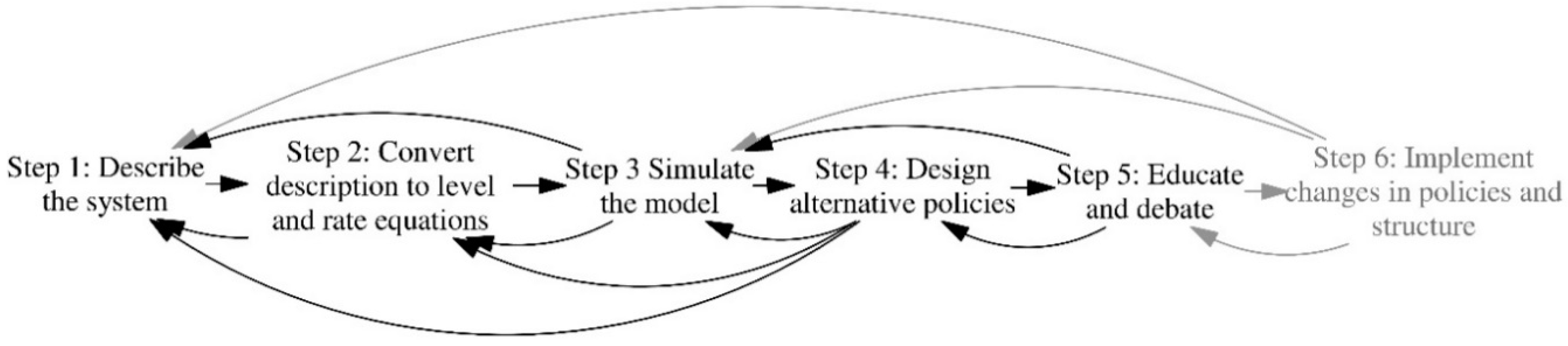
Our research follows the iterative process in
Figure 1, which characterises that the system dynamics combine aspects of qualitative and quantitative research [
8]. The first five steps are relevant for the purposes of the research as the implementation of changes (sixth step) constitutes a farmer’s responsibility.
The whole process started with interviewing farmers [
4,
57]. For these purposes, we applied the focus group interview method [
58], which is well suited for a sample population with homogeneous characteristics [
59]. Addressing the topic by the focus group interview method elicits the interaction and discussion, which strengthen the quality of generated responses [
60,
61]. This led to forming a dynamic hypothesis [
11] into a causal loop diagram, which identifies the main feedback loops. At this stage, CATWOE (Customers, Actors, Transformation process, Worldview, Owner, Environmental constraints) from the soft system methodology [
62] was also adopted to help formulate the model boundary, systemize the farmers’ opinions, and ensure that the model reflects all appropriate elements. This stage is important to form the model structure and to reach the crucial “mental database” of farmers’ [
12] (pp. 143–144).
According to the interviews, we have defined the model assumptions that are reflected in the model structure and tested scenarios. The small cattle beef production is modelled and simulated according to the decision making common to the farmers. The production—breeding, capacity changes, and slaughtering—is aimed to maximize the profit from meat, however, the farmer cannot influence the prices of inputs and outputs. Farmers are dependent on the subsidies that represent the high share of their income. Farmers’ satisfaction (being the farmer) and family tradition are frequently superordinate to profitability. Family members often replace the paid stuff. Therefore, farmers could stay in the market when the situation is undesirable and subjects in different market areas would have already left or been bankrupted.
One of the advantages of system dynamics approaches in comparison with other modelling approaches is the deep understanding of interconnections between the elements of the system and feedbacks that arise from these interconnections [
63].
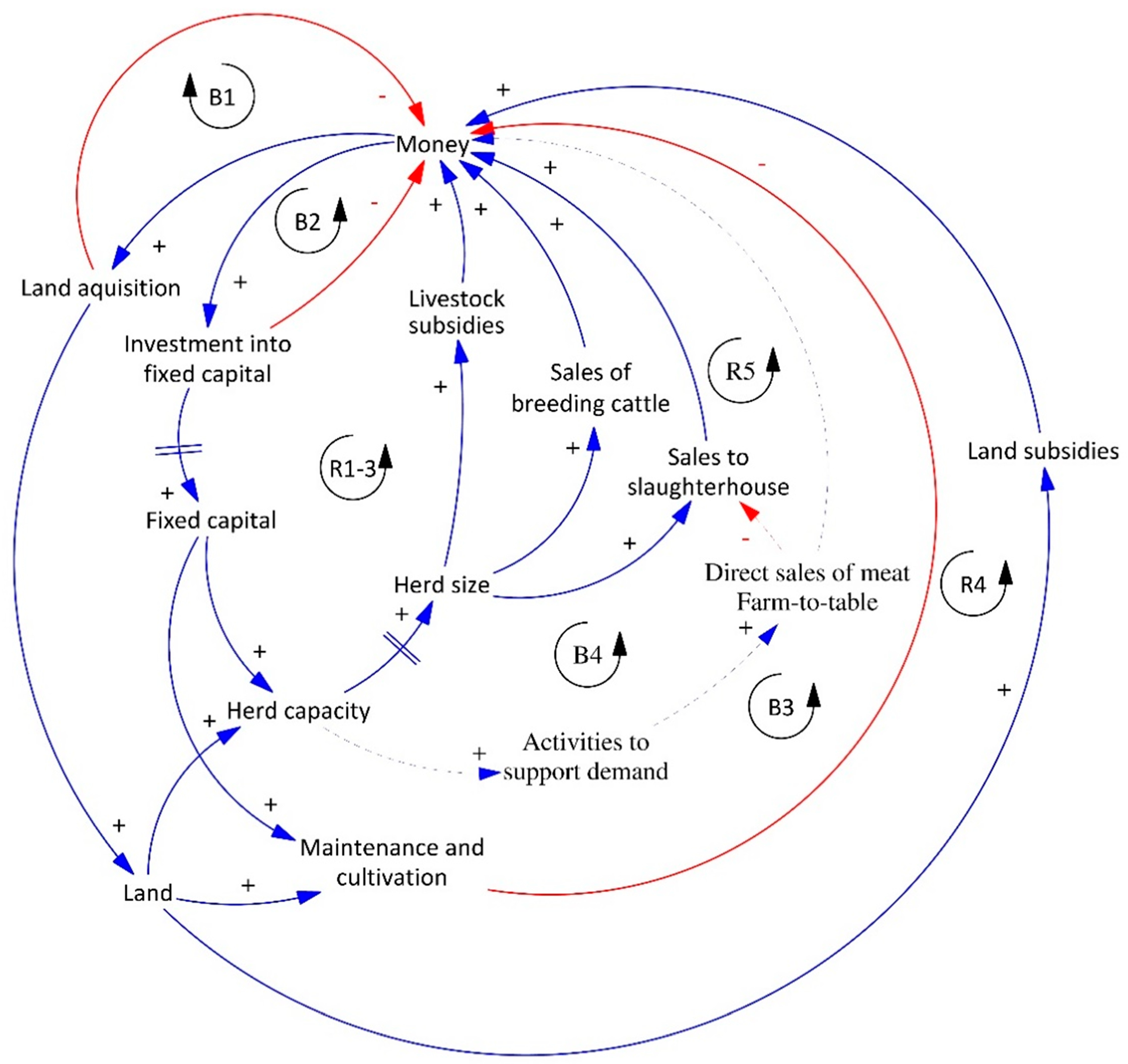
Figure 2 shows the main drivers and feedbacks of beef cattle farming identified during the interviews. The aggregated high-level causal loop diagram (CLD) summarises the main links among the core characteristics of a farm. CLD serves as a starting point of the modelling process that allows capturing the farmers’ mental models and expresses a hypothesis about the sources of the farm management dynamics.
The plus (+) sign denotes positive polarity, that is, that if the independent variable increases the dependent variable increases above what it would be. It also means that the dependent variable decreases when the independent one decreases. On the contrary, the negative link polarity expressed by the minus sign (−) denotes that if the independent variable increases, the dependent variable decreases below what it would be. Similar to the positive polarity, negative polarity also captures the opposite behaviour of the independent variable—if the independent variable falls, the dependent variable grows. See Richardson [
64] and Sterman [
11] for details on the interpretation of CLD.
The source and driver of the behaviour of a system is its structure [
10,
65]. The dynamics arise from the feedbacks denoted in
Figure 2 as R for the reinforcing and B for the balancing loop. The loop denoted as R1–3 stands for the main source of income from beef cattle breeding—money from slaughtering, suckler cow subsidies, and sales of cattle for breeding. All three incomes grow with the size of the herd. This drives the reinforcing loop through the investment into land and fixed capital (mainly buildings and machinery), which together represent the maximum capacity for the herd size. The parallels crossing the causal link express the delay that is common for the extension of a herd if a farmer does not buy new cattle from others. These extensions lower the available resources via expenditures on the investment (B1 and B2) and via continuous maintenance and cultivation (B3). Although the land subsidies are not strictly connected with livestock production, farmers consider R4 as a significant driver of the farm’s performance.
Loops B4 and R5 are specific only for the farmers that diversify into meat processing and distribute their products directly to the final consumers (dotted causal links in
Figure 2). This strategy drives the income from R5 and counteracts the reinforcing income loop that leads through the sales to slaughterhouse.
However, the discussion with the farmers and the application of CATWOE identify the limits of the reinforcing loops, which are unique for agriculture. In the soft system methodology, the CATWOE part usually enriches the root definitions and conceptual models [
62,
66]. For our purposes, we use the approach in the problem structuring phase to define the main stakeholders and elements of the system [
67,
68], which results in the definition of the model boundary.
Table 1 summarises characteristics of the system in CATWOE framework—originally used for the proper formulation of root definitions [
62], which helps to systemise and express the farmers’ ideas of the reasons for cattle farming and the current situation in the field. This soft method produces results based on mental models of the current participants. If the participants were switched for the main actor in the market or CATWOE was built for the whole cattle breeding sector of the whole country, the characteristics would differ significantly.
The final row in
Table 1 clearly illustrates the market position of small farmers and influences the model design. Environmental constraints in CATWOE include important factors and limits that are considered given for the described system; they are out of the reach from the inside of the system. Small Czech farmers have minimal influence on the prices of both inputs and their own products. Fousekis et al. [
69] describe a similar situation in the United States, where the wholesalers benefit from an advantage over primary producers in the beef sector. Moreover, farmers often cannot decide on the time and size of their own expansion because the core resource—the land—is unavailable at their convenience. Instead, they acquire land when it is available.
These facts have an impact on the modelling of the reinforcing loops from
Figure 2 and the model boundary in
Table 2. The growth possibility connected with the acquisition of land and buildings is naturally an exogenous variable for small farmers. The model boundary [
70] summarises the most significant endogenous, exogenous, and excluded variables.
Despite that some authors find the causal loop diagram sufficient solution for specific types of problems [
71,
72], the core system dynamics’ tool to overcome the limits of human capacities to deal with complex problems [
11] and, therefore, the important step in the process of system dynamics approach is the creation of simulation model [
53,
73]. A further development and extension of CLD in
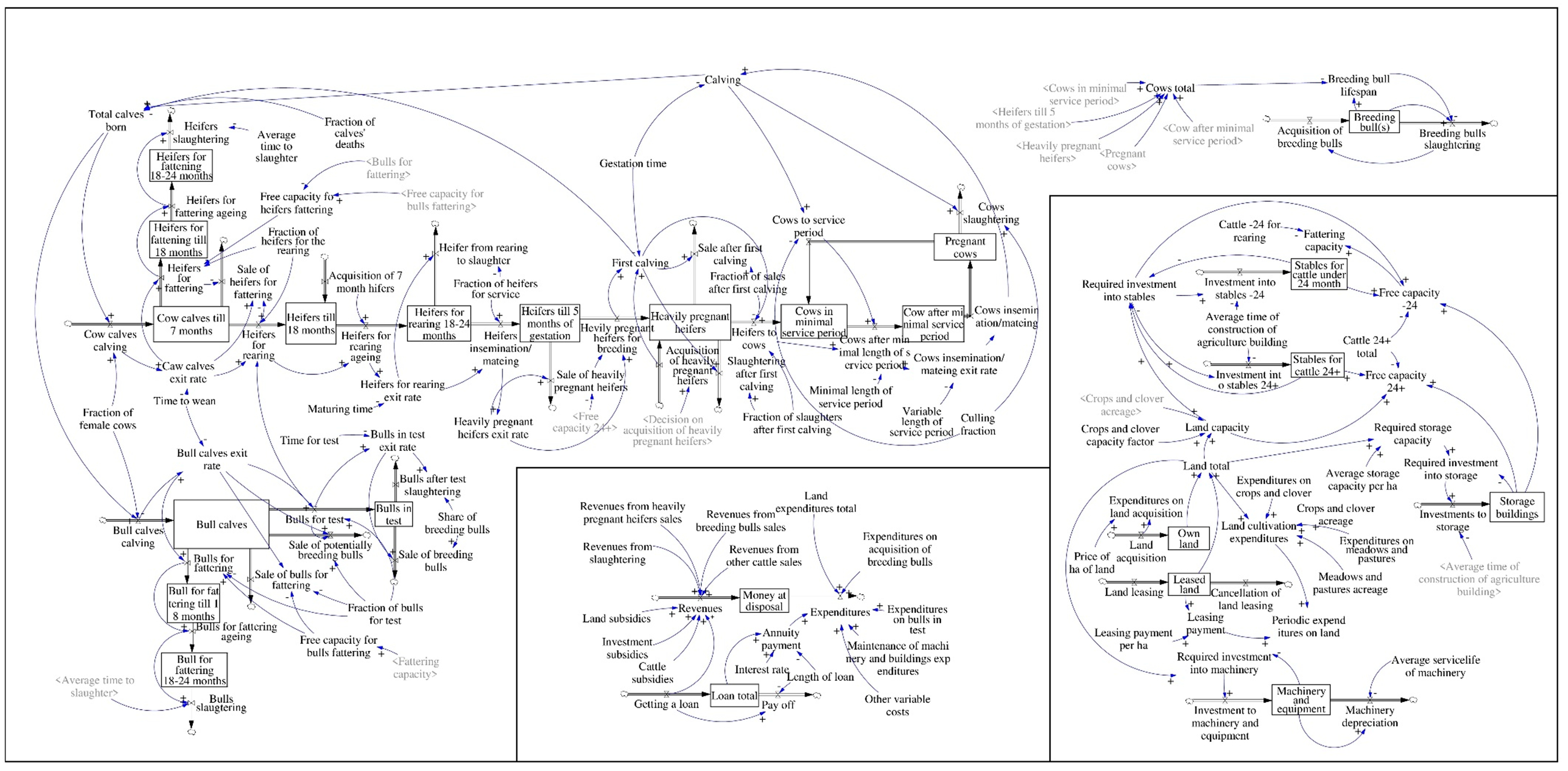
Figure 2 leads to the stock and flow diagram (SFD) in
Figure 3, which is closely connected with step 2 of the system dynamics process—conversion into equations—and constitutes the management flight simulator. The interpretation of link polarities remains similar to the CLD. The clear mathematical expression of the positive link is then defined in Equation (1):
Equation (2) shows the general mathematical expression of the negative link:
where
x expresses the independent variable (at the beginning of the arrow) and
y is the dependent variable (aimed by the head of the link arrow). The box variables represent stocks (levels) in the system and are mathematically expressed as definite integrals (3):
where
s represents a stock variable,
i comprises all inflows,
o includes all outflows, graphically denoted in SFD by pipes with faucets leading into the box variable or out from it,
T0 is the initial time,
T constitutes the current time, and
t is any time between
T0 and
T. See the work of [
11] for an in-depth explanation of stock and flow diagrams.
Figure 3 shows the SFD of the main subsystems of beef cattle farming. This phase requires parametrisation, and thus collecting data from farmers. Many small farmers take the opportunity of high flat-rate taxation, which makes accounting simpler. However, it results in a lack of data on the economic subsystems of the given farms. The top part of
Figure 3 shows the core of a farm and our model—the structure of the herd, which is represented by only one variable in
Figure 2, is developed into the form of two interconnected ageing chains. Such a disaggregation of variables representing the herd structure has two reasons. Firstly, it increases the trust of the farmers in the simulation model as they can see that the modelling structure represents the main characteristics of their herd. Secondly, the time series data on the livestock structure are usually well documented. Therefore, it is possible to test the quality of the model on this subsystem and calculate the missing parameters.
The bottom right part of
Figure 3 represents the simplified structure of fixed capital. Land constitutes the main variable. The possibility of buying or leasing land naturally represents an exogenous variable for farmers. Therefore, the volume of other capital stocks (machinery, stables, storage, and other non-residential buildings) depends on the land area at a farmer’s disposal. Typically, three factors limit the overall herd capacity—land area, stable capacity, and storage capacity. Stables are split into sections for cattle below 24 months old and cattle over 24 months of age. However, the land and storage capacity use coefficients for various age categories of cattle from the herd structure subsystem. The service life of buildings and machinery arises from the parameters of the perpetual inventory method for estimations by the Czech Statistical Office [
74]. For the cases of missing data concerning the construction period, findings from two databases were used (the business register and the statistics of building approvals). The average construction period of buildings for animal production amounts to 2.99 years [
75].
The central bottom part of
Figure 3 shows the economic subsystem of a farm. A diagram of this structure requires aggregation of the inputs (e.g., revenues from slaughter come from various variables of herd structure) to remain readable.
The model describes the main characteristics of a farm in a dynamic form and evaluates the impact of decisions on a farm’s future performance. The system dynamics approach allows evaluating a “what if” analysis [
11,
76]. The management flight simulator enables the ability to design, test, and evaluate the impact of various scenarios and strategies. The model simulates the consequences of decisions and changes of environmental conditions in time. A comparison of the development scenarios allows choosing the most efficient strategy subject to given conditions.
For the first part of the analysis, we create the theoretical model cattle farm. The herd consists of 100 animals in total where the shares of the categories are in equilibrium. These shares were obtained from the simulation of 1000 randomly generated herds. All these artificial herds converged to the equilibrium structure. Other data were mostly obtained from the Institute of Agricultural Economics and Information [
77] and Czech Statistical Office [
38,
78], and from interviews with farmers, the summary of the model settings with the specification of the source for the individual parameters is in the
Appendix A Table A1. Then, we compare the scenarios of capacity extension and the impact of the farm-to-table strategy. In case the scenario’s circumstances require the identification of the best solution, we apply the Powell optimization [
79,
80] with multiple starts (10 vector points).
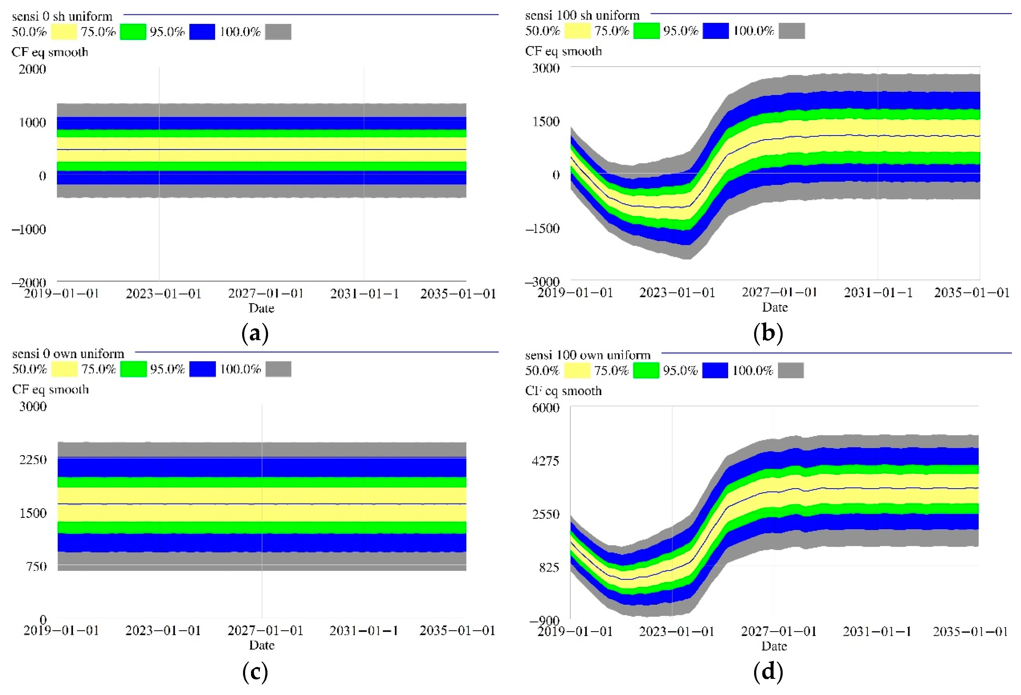
The system dynamics models adapt the sensitivity analysis to deal with the uncertainty of the parameters and to identify the impact of the parameter change on the system behavior [
81,
82]. The sensitivity analysis is in the
Figure A1 and
Table A2 followed by the summary of the model testing.
From our previous research [
4], we know that there is usually nothing like the “average farmer” and, despite that the statistical data describe the situation in the country very well, the simulation based on these data does not provide the answers on questions of individual farmers with the specific real-life problems. In a different field, the research underutilization is called the “know–do gap” [
83] (p. 2), and it is well known that “the passive dissemination of information was generally ineffective in altering practices no matter how important the issue or how valid the assessment methods” [
84] (p. 466). The movement towards the strengthening of the implementation methodology and case studies is observable [
85]. Therefore, the last part of the results presents the real case study of a selected farm in the Plzeň Region. The owner agreed with the presentation of the results. That specific farm was selected because it allows evaluating the impact of various development and growth scenarios. The farm was founded in 1990 and focuses on the production of Beef Simmental. The farm represents the archetype of growth inefficiency caused by dynamic complexity, but also utilises some of the possible improvement opportunities. The specific of the farm rests in the realisation of farm-to-table strategy since 2011. Various scenarios are compared and the impact of diverse decisions on the farms’ performance evaluated after an extension of the herd maximal capacity from 54 to 174 in 2009 (for all cohorts from
Figure 3). This significant extension resulted in a necessary reconstruction of stables in 2016 supported by investment subsidies, but also in a bank loan of nearly 75 thousand EUR with a 20-year maturity. The parameters of the demonstration farm are in
Table A3. The case study documents the benefits of the farm-to-table strategy, but also shows the possibilities of computer simulation when managing the dynamic complexity of beef farms.
3. Results
3.1. Farm-To-Table in Comparison with the Farms’ Capacity Extension
This section describes possibilities of the management flight simulator in the environment of a beef cattle farm and expresses the shift of the economic situation of a farmer that realises the strategy of direct delivery to final consumers. The presented results represent the outputs of steps 3–5 of the system dynamics process from
Figure 1. The first part presents the theoretical model that is set to 100 animals in equilibrium structure, which could be simply revaluated into percentage or recalculated to the different size of the herd as a ratio to the real farm herd.
The simulated scenarios were focused on the extension of the farm capacity (land, stables, and storage capacity) under three different circumstances:
The scenarios were selected according to the research question and compare and evaluate the impact of farmer’s effort to improve the economic situation via reinforcing loops R1–3 and R5 in
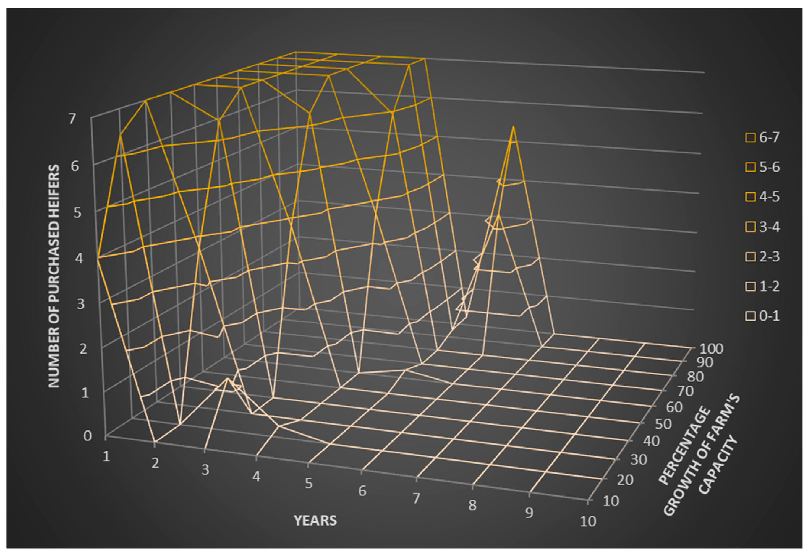
Figure 2. The result of the farm’s capacity extension could be significantly influenced by the acquisition of the cattle to the herd, which has an impact on the time of capacity utilisation. Therefore, we also added the evaluation of optimal acquisition of heavily pregnant heifers.
The main tracked variables are the number of cattle older than 24 months, because this part of herd determines the other categories and measures the extent to which the farm’s capacity actually extended. All categories of herd are measured by the number of heads. Only in cases of capacity utilisation and specific subsidies in case studies, we use life stock coefficients [
86]. For the description of the farm’s economic situation, we selected the cash flow in EUR/month. The farmers have often insufficient bookkeeping data—the cash flow is simply connected to flows in the herd and the indicator is close to the farmer’s understanding of money they have at disposal.
To avoid the instability and oscillation of the herd structure [
87,
88,
89], the optimal purchases of the heavily pregnant heifers were limited by the culling fraction (7%). The objective function was set to maximise the aggregated cash flow revaluated to prices of 2016. The course of the optimal purchases of the heavily pregnant heifers according to the percentage growth of the farm’s capacity is in
Figure A2 and
Figure A3. For these scenarios that evaluate the future development, we revaluate the parameters that express the prices of inputs and outputs by the 10-year average inflation (1.9%) [
78].
The initial simulations were focused on the dynamics of the capacity extension, especially on the delay between the extension and full realisation of the benefits of the extension. The extension of stables, land, and storage capacity in cattle farming is subject to the long periods of natural turnover, but could be supported by the acquisition of cattle from the other farmers. The extension of the small-scale farm is usually problematic because of the inability of the farmer to decide when to expand. The management simulator could provide the efficient tool to measure the result of various strategies and identify the optimal one.
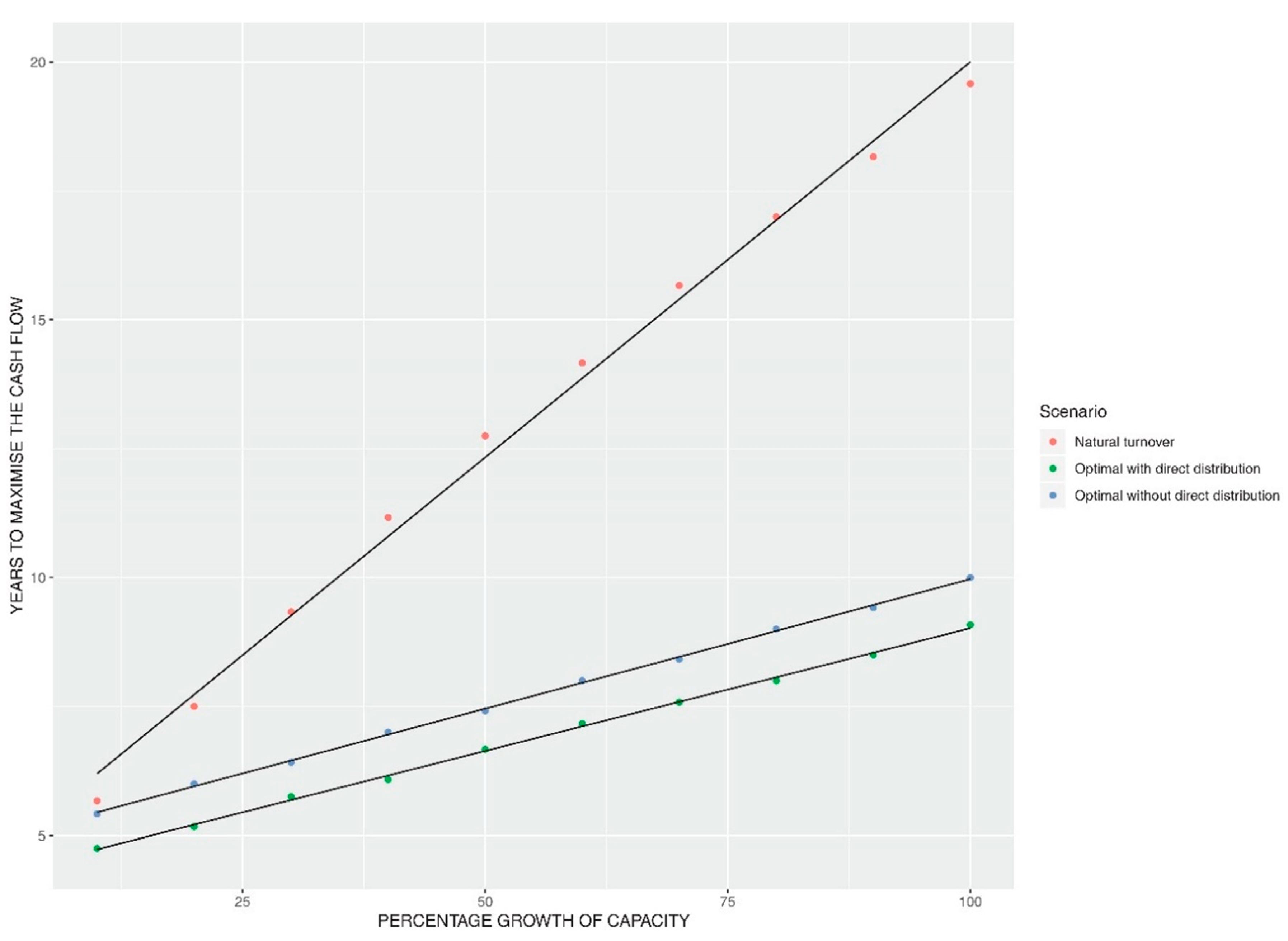
Figure 4 shows the dependency between the percentage extension of the farm capacity and years from this extension to the point when the farm reaches the maximal cash flow. The time of natural turnover is nearly double in comparison with the situation when the farmer optimise the heifers’ acquisition. The time to maximise the cash flow could be even lowered if the farmer realises the farm-to-table strategy (scenario called “Optimal with direct distribution” in
Figure 4). Parameters of the functions, expressing the relation between the capacity growth and the time that is necessary to reach maximal possible cash flow, are in
Table A4.
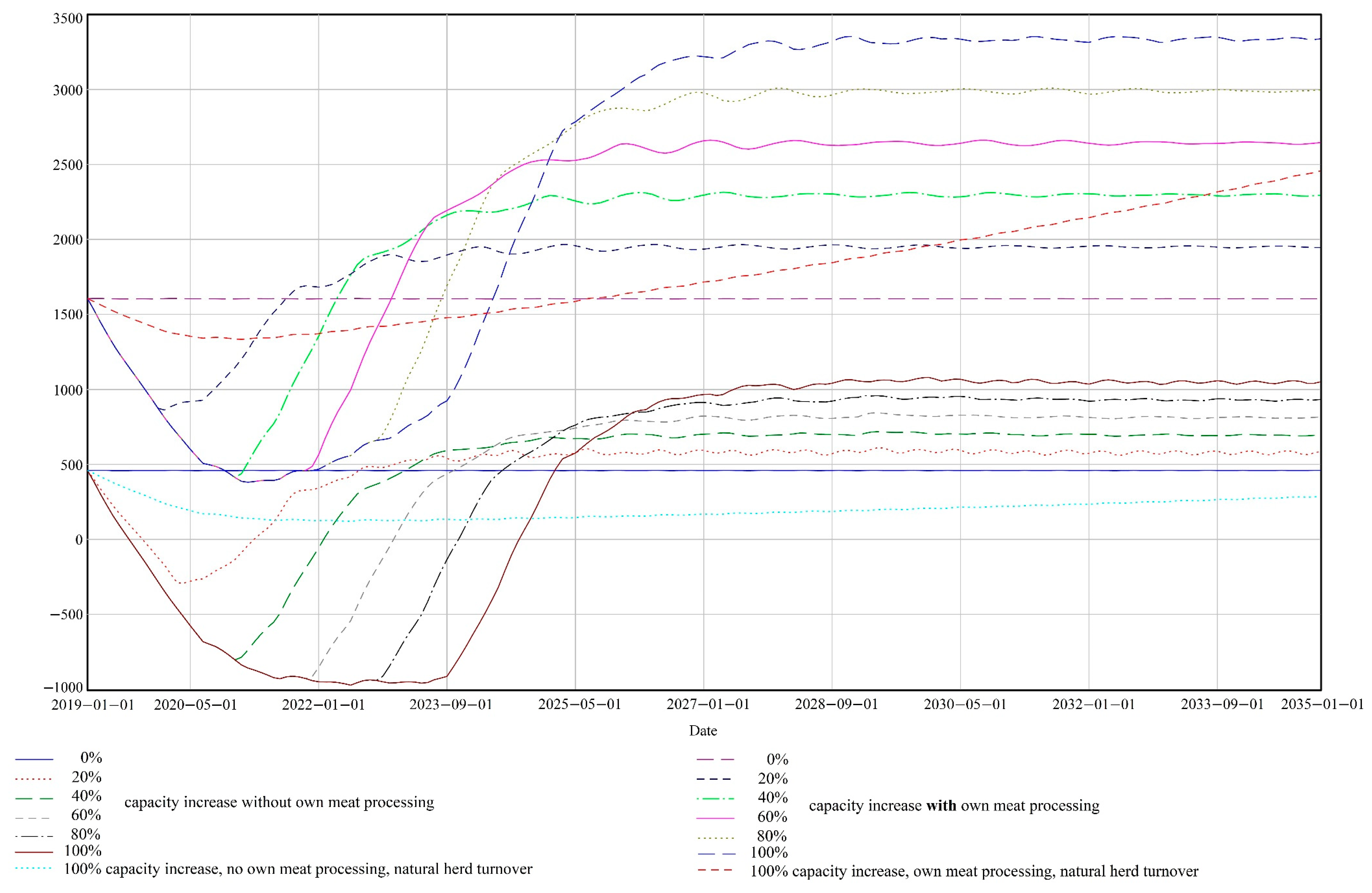
Figure 5 shows the development of the cash flow under selected extension scenarios. The scenarios differ in percentage extension of the farm capacity (0%, 20%, 40%, 60%, 80%, and 100% increase) and evaluate the situation from the perspective of the common farm and the farm that diversifies into direct sales of the meat to final consumers. The graph is visibly divided into two parts, where the higher bunch of lines describes the development of cash flow in conditions of own meat processing the lover part represents the situation when the farm sells the cattle to the slaughterhouse. For comparison, the graph contains two lines representing the 100% increase of the capacity with natural herd turnover.
The initial decrease is caused by heifers’ acquisitions, but also by the decrease of sales of cattle for rearing, which would be sold in the case of full capacity, but enter the herd after the extension. According to the model assumptions, the model does not contain the bankruptcy structure, however, it is clear that the significant capacity extension should be accompanied with the extension of the herd by acquisitions of the heavily pregnant heifers. However, the revenues from cattle for slaughtering could not cover these expenses. Especially, in the case of farms that sell the cattle to the slaughterhouse, the cash flow could fall to negative numbers for a long period. The farmer must take this into consideration during the preparation of the subsidy and loan requests. The figure depicts the benefits of direct sales of meat to final consumers. Even the 100% capacity extension does not reach the level of the farm’s cash flow without that extension, but with the own processing and distribution of meat. The cash flow of the theoretical farm with direct distribution of the meat to final customers reaches the level between 1602 EUR/month and 3353 EUR/month depending on the simulated scenario (total capacity 100 vs. 200). The farm that sells the cattle to the slaughterhouse (which is a dominant strategy in individual cattle farming) reaches the cash flow between 459 EUR/month and 1081 EUR/month.
Under the given circumstances, the capacity extension of the farm that sells the cattle to the slaughterhouse must be more than 170% to reach the cash flow of the farm that does not increase the capacity size, but realises own meat processing and distribution. Similarly, the cash flow of the farm that sells the meat to final consumers falls to the level of the farm with double capacity size and sales cattle to the slaughterhouse when the average price of meat falls to 81.3% (135.8 CZK/kg) of the actual average price.
The farm-to-table strategy provides both higher and earlier maximal earnings in the case that the farmer has the possibility to expand the capacity. Moreover, the higher cash flow also facilitates the optimal heifers’ acquisitions as the bottom of the cash flow during the highest purchases falls only to the level that is common for the farmer processing the meat.
3.2. Case Study
This section describes the application of the management flight simulator on the selected beef cattle farm that illustrates the impact of the farm-to-table strategy on economic sustainability of the farm. The significant difference to the previous section is that the costs are not only an average value per cattle, but the model contains the fixed expenditures and variable expenditures relative to land and other fixed capital. There are also delays between individual investment decisions (e.g., differences in time of acquisition of land and stables), which are common in real farm management.
A comparison of six selected scenarios is provided, illustrating the current situation of the farm, evaluating the decision of the farmer to process meat and identifying future steps that lead to full utilization of stable capacity. The six scenarios compare the results of the application of direct sales of meat to final customers with sales of cattle to the slaughterhouse. Both approaches are compared under the circumstances of real capacity extension. The other scenarios evaluate the impact of the heavily pregnant heifers’ acquisition. The scenarios reflect the effort of the farmer to enhance the economic situation of the farm via the reinforcing loops R1–3 and R5.
The scenario “Basic” follows historical time series. The stable capacity increased to 174 cattle (of which 64 are supposed for cows of age 24 months and more) in 2009, but the land area remains equal to 104.5 ha until 2017 when the leasing opportunity allows the increase of the land for farm’s purposes to 147.5 ha. After the stable extension, the farmer purchased five heavily pregnant heifers in 2010, two heavily pregnant heifers in 2012, and three more in 2015. The farmer stands out because of vertical diversification. The farmer stopped selling cattle to a slaughterhouse in 2011, contracted a butcher, and sells the meat himself instead. Thus, the whole process of producing meat remains under the farmer’s control and such a decision led to an increase in the farmer’s selling prices with a minimal need for initial investment. However, the farmer also takes the responsibility for the existence and satisfaction of customer demand. The basic scenario contains no future cattle purchases or expanding the herd via natural reproduction.
The comparison of the scenarios arises from the accumulation of cash flow measured in EUR/month respectively aggregated cash flow measured in EUR.
Table 3 summarizes the list of scenarios presented and compared for the case study. The last column contains the difference between basic scenario (farmer realises the direct distribution to the final consumers, but does not buy other heifers) with other simulated scenarios. The constant difference is caused by the late capacity utilisation, and the variable difference is caused by the different strategies, where the farm outputs can’t reach the same levels.
Figure 6 shows the two main indicators that represent the performance of the farm under the conditions of the six scenarios—the number of cows older than 24 months (
Figure 6a), which represents livestock and main production capacity and aggregated cash flow before the subtraction of farmers’ family earnings (
Figure 6b).
To increase the sales, the farmer supported the sales of the meat by additional services. At the beginning, he provided cooking courses focused on the beef preparation. However, as these courses raised to be common in many restaurants, he changed the support services that reinforce loop R5 from
Figure 2. The farmer also neglected the participation in farmers’ markets, which are supposed to support the distribution of small-scale farmers’ products. However, the farmer finds it too expensive and with very small value added. Nowadays, the services are focused on pedagogy, where clients (mainly kids) experience taking care of cattle or, for example, flail the crops. Nevertheless, the demand for the beef already reached the level that the farmer does not face the problem of unsold meat. The support services were implemented into the model as a very simple structure from
Figure 7.
Diversification as an Opportunity
The scenario called “Without meat processing” follows the same steps as the “Basic” scenario, but omits the diversification. The difference between these two scenarios expressed in aggregated cash flow amounts to more than 56.9 thousand EUR in the period from 2011 to 2018. As the size of the herd and the number of cattle for slaughter grows along with it, the annual difference increases, too. The aggregated difference would come to more than 149.9 thousand EUR in 2025 and 242.7 thousand EUR in 2030.
The scenario titled “Double historical purchases” shows a theoretical development of what would happen if the farmer doubled the acquisitions of heavily pregnant heifers after 2009. The prices of heifers varied between 1100 and 1300 EUR per heifer in the period from 2010 to 2015. Such a decision would lead to faster capacity utilisation and, therefore, earlier maximisation of outputs and income as a consequence. This scenario predicts the capacity of 64 cows older than two years being reached by 2030, while the basic scenario reaches that maximum seven years later. After 2037, the output and earnings of these runs reach the same level; however, this seven-year gap would result in the difference of 479.3 thousand EUR of aggregated cash flow. The difference in time when the farm reaches the maximal capacity proves even more important as 2037 represents a breaking point from the expense point of view. The capacity expansion came with the necessity of the bank loan, due in 2037. Therefore, reaching the maximal outputs before that year eases the pressure of dealing with the loan payments.
The scenario remains theoretical as the historical decisions are given. Therefore, simulations were performed with similar results, but with a focus on future decision making. To prevent getting an overly optimistic scenario, the highest purchase price from the real purchases since the stable extension was used. The price amounted to nearly 1300 EUR per heavily pregnant heifer in prices of 2015. The costs are revaluated to current prices of the given year on the basis of historical price indices and the five-year average percentage change of the prices for the future estimation.
Various scenarios of quantity and frequency of purchases were tested for these purposes. In the scenario titled “Future purchase5”, the farmer acquires five heavily pregnant heifers each year until 2022. Under these conditions, the capacity of cows older than 24 months is reached in 2025. Such purchases are still achievable without a significant effect on the cash flow throughout the period of heifer purchases and lead to similar earnings to the “Double historical purchases” scenario by 2026. Larger purchases before 2022 would result in earlier maximisation of annual earnings, but the necessity to keep the annual cash flow at a level still securing the income of the farmer’s family should be considered. On the other hand, lower acquisition of heifers would result in a lower aggregated cash flow in comparison with the “Double historical purchases” scenario. The difference between the aggregated cash flow of this scenario and “Basic” reaches nearly 535.6 thousand EUR.
The scenarios “Basic+” and “Without meat processing+” project the real pattern of heifer purchases of the farmer into the future. These scenarios assume that the farmer continues the purchases. Therefore, the model simulates the heifer acquisition policy similar to the period after the stable extension. Both scenarios simulate the purchases of three heavily pregnant heifers every two years until 2026. The difference between these two scenarios corresponds to the difference between the first two: “Basic+” contains the diversification, “Without meat processing+” does not. The right section of
Figure 4 shows that in the long term, even the “Basic” run without any further purchases of heifers is more profitable than “Without meat processing+”. These scenarios estimate reaching the capacity in 2029. The difference of aggregated cash flow between the “Basic+” and “Future purchase5” scenarios then amounts to nearly 179.2 thousand EUR before the flows of outputs and earnings reach an equal level. In comparison with the biggest investment in the farm’s history, this sum represents 64.7% of the total price of the stables acquired in 2009, including the reconstruction expenditures in 2016 (after revaluation of all figures into the prices of a single year). The impact of such income on the budget of the farm increases considering the fact that the acquisition of stables was supported by a 60% investment subsidy. Consequently, the aggregated difference revaluated into the prices of 2016 represents 162% of the expenditures from the farm’s own sources (including the bank loan) connected with the acquisition and reconstruction of the stables.
The diversification in terms of farm-to-table strategy decreases the dependence on subsidies as the share of the non-investment subsidies falls from over 37% to less than 32%. If the farm does not realise the meat processing, the annual cash flow could grow from 15.6 thousand EUR in 2018 when the capacity is not fully utilised to nearly 84 thousand EUR when the herd reaches the full capacity. On the other hand, the current annual cash flow could grow from 29.7 thousand EUR to more than 112 thousand EUR after reaching the full herd size in the scenarios where the farmer looks for a solution of the weak position of a primary beef producer and realises the benefits of diversification. The difference of income from slaughtering between these scenarios reaches the 45.3% of non-investment subsidies. Also, the fixed asset turnover [
57] grows from 9.6% without the farm’s own meat processing to 10.9% when the farm processes, stores, and sells the meat.
The case study is the example of the farm-to-table strategy as a growth driver that significantly improves the economic situation of the farm, which is tightly connected with the viability and economic sustainability of the farm. The farmer actively grows through all main reinforcing loops, however, it is clear that the R5 for diversification is the one that increases the efficiency and changes the farm’s position. Despite the right decision of the farmer, which was made intuitively, the management flight simulator still proves to be an efficient tool to improve the growth strategy, because the low heifer acquisition delays the full benefit from the capacity extension.
4. Discussion
The structure of a system represents the source of its behaviour [
10,
65]. The presented dynamic model simulates beef cattle production from the perspective of individual farm management. The application of the system dynamics methodology enriches the understanding of the beef cattle farm system and provides a tool for a
what-if analysis. Although management and economic evaluation of the farm represents the main goal, from the systemic perspective a modeller must consider the physical structure of the herd as a core subsystem. The physical structure of the herd with the biological processes, limitations, and delays determine the behaviour of economic subsystems of the farm. Moreover, the herd structure was proven to be an efficient indicator for model validation because farmers could provide the best real data series on the herd.
A modeller’s ability to transform an economic and agricultural problem into a mathematical form limits the benefits of simulation models [
27]. Moreover, the methods of hard system thinking (including computer simulation) have the disadvantage that a modeller could “lose touch with aspects beyond the logic of the problem situation” and problem owners [
62] (p. 765). To prevent that, the whole process started with the interviews and farmers’ participation in the model and indicator specification [
57]. The mental data prove to be crucial for the understanding of the system [
11,
12] and would remain inaccessible without direct cooperation.
Some of the simulated scenarios show the trap of the weak market position of primary producers in the beef sector [
40,
69]. The case study was selected in order to show an opportunity for a small farmer to escape the position of a mere primary producer. The simulated scenarios allow the ability to clearly quantify the benefits of vertical diversification when the farmer enters the meat production and distribution sector. Sale prices are commonly identified as the most significant aspect for the profitability and margin value per ha [
40,
43]. However, a small producer lacks the market power to change prices. Meat processing constitutes an opportunity for participating in the advantage of beef packers. In the presented case study, the income per one slaughtered cattle increased by 50.2% or 76.3% depending on the gender of the cattle. The annual cash flow consequently grows by more than 33% upon utilising the full capacity in situation of the case study and even more if we use the official statistics on average values of the parameters.
Because one of the fundamental modelling principles is that the modellers should always model a problem and never the whole system [
11,
73], the model does not directly deal with the topic of high greenhouse gas (GHG) emissions, which are a typical undesirable effect of cattle farming [
90,
91]. Nevertheless, in comparison with the simple growth of the herd size (which means the increase of emissions), the farm-to-table strategy significantly improves the economic performance of the farmer. Therefore, the farm-to-table represents the strategy that improves the economic sustainability that is not accompanied by the direct negative effect on environmental sustainability.
The lack of opportunity to acquire more land frequently limits the growth possibilities of a farmer. If the growth of the land area and facility capacity arises, the farmer must not underestimate the investment into the herd. Agribusiness is specific for long delays that cannot be altered as they are essential for biological processes [
16,
17]. From this perspective, the growth of the herd size depends on the natural reproduction process. In the case of a significant extension, natural reproduction fails to fill the capacity before the maturity of the long-term loan, which—on the other hand—proved necessary for the investment into capacity. In other words, the investment does not attain its full utility and the revenues do not reach the possible level during the period of increased expenditures because of debt payments.
Underinvestment was the topic for the system dynamics approach from its origin [
92]. “Growth and underinvestment” also constitutes one of the system archetypes, that is, common patterns of behaviour that occur in various fields and carry some typical (archetypal) problem [
9]. Behaviour produced in a system archetype is a kind of a trap. Nevertheless, if a manager identifies an archetype, it could be considered as an opportunity [
10]. Timely investment into the herd size allows the farmer to fully utilize the production capacities and reach the maximal level of income earlier. The economic strategies are commonly considered to affect mainly short-term farming sustainability [
1], however, this is dependent on the farm’s main product. The cattle farming is typical for its inertia and the long-term impact of decisions made by farmers. For small businesses, the survival of the growth phase could be very problematic [
93,
94,
95]. The farm-to-table shows to be the leverage, which significantly increases the economic efficiency and, therefore, the viability of the farm. From the system dynamics point of view, the change of the constants is usually considered to be the weakest leverage (change relative to the effort) in comparison with any change in the structure of the system [
10]. The change of the maximal capacity represents this kind of low leverage parameter change, on the contrary, the farm-to-table strategy is the change of the structure with a higher impact on the behavior of the system.
Small farms within the EU mostly represent a family activity [
3]. This fact brings two important aspects. Firstly, many operations are carried out on a part-time basis and the given family often needs an additional source of income. Secondly, the decision to run a farm often arises from a family tradition [
4]. Despite small farms being considered the cornerstone of the EU agriculture, the weak market position of small farmers might work as a barrier to entry for new farmers or a demotivating aspect for the new coming generation at existing farms, that is, a generation change. Therefore, when traditional farmers quit, their replacement by new small entrepreneurs may never come. Sustainable development of the EU agriculture stands as the Priority of the EU Common Agricultural Policy for 2021–2027. Support will focus on small and medium farmers [
2]. This might help to improve the situation. However, system dynamists also know a system archetype called “Shifting the burden”. The archetype stands for problematic behaviour arising from dealing with symptoms instead of providing a fundamental solution [
9]. Subsidies might be a different case, but a higher share of subsidies in the income increases the dependency on a source outside the farm system, that is, again something that the farmers cannot change. Complex systems are hard to understand and predict. However, being passive in a complex system is not a solution. For these purposes, the management flight simulator used in this work was designed to allow active testing and analyses of the long-term impact of decisions made by a farmer.
Our further steps in this research will address other types of animal production. Implementing a user-friendly interface to the simulator constitutes a crucial issue. Such an interface represents a necessary move towards acceptance and adoption of the simulator by farmers. Moreover, the user interface allows the farmer to use the management flight simulator without the need for personal guidance of members of our research team. The farmers’ trust is a precondition of the sixth step of the followed process, that is, real implementation of changes.
5. Conclusions
The presented study depicts the issues of beef cattle farmers in the market environment and illustrates the benefits of management flight simulators for cattle farming. Describing beef cattle farming as a dynamic complex system helps to understand the sources of behaviour and the resistance to applied strategies and policies. The common complexity of managing a company is further complicated by biological processes characterized by very long time periods, especially in the case of beef cattle farming. Moreover, the impossibility to affect the prices of inputs and outputs pushes farmers into a passive role. A computer simulation represents a tool developed to help understand such complex systems.
In the results, we evaluate the effect of direct distribution of meat to the final consumer on the economic viability of small-scale farms. The implemented management flight simulator allows expressing the difference between a pure primary producer and the farmer who decided to participate in the advantage of retailers. Considering the growth strategies, the farm-to-table shows to be strong leverage:
Farm-to-table strategy significantly increases the cash flow of the farm.
Farm-to-table strategy enables earlier utilization of the capacity extension.
Farm-to-table strategy allows the growth independently on the exogenous variables, which limits the capacity growth (especially the possibility of land acquisition, cost of the land, annual rent per hand subsidies).
We also simulate and evaluate various scenarios that show the benefits of early investment into the herd size when the maximal capacity of stables increases. In the case of cattle farming, even the single discrete economic/managerial decisions influence the farm’s viability in the long term. Delays connected with biological processes hold-up capacity utilisation in the growth phase of the farm. In the case of significant capacity extension, this delay could result in late maximisation of earnings, which could be reached only after the period of maturity of the relevant bank loans.
The capacity extension must be accompanied by the proper acquisition of heifers. Relying only on natural reproduction of livestock might result in significantly lower cash flow. Appropriate acquisition of cattle works as a significant growth driver that allows earlier maximisation of the farm’s output and accelerates the return on the initial investment.
Small farmers in the role of pure primary producers hold a significantly weak market position owing to the impossibility to influence the prices of inputs and outputs. Although proper cattle acquisition in the extension phase results in better income in the long run, it fails to change the market situation and the farmers’ dependency on the decisions of others. Diversification into processing and own distribution of the meat, on the other hand, represents an active strategy that mitigates the mentioned primary producers’ risks and increases the cash flow and fixed asset turnover. From the perspective of economic sustainability, the farm-to-table strategy shows to be significantly more efficient and sustainable than the capacity extension.
The limits of the model rest in the environmental and social sustainability, as the model does not provide the indicators for these dimensions. The reader must also understand that despite that the farm-to-table strategy could be very efficient, it is also a subject of farmers’ knowledge and skills together with the willingness of the farmers to leave the comfort zone of doing what they do for years. The strategy is also restricted by the regional demand for such products. As the model focuses on individual farms, it does not work with the demand curve, which would be necessary if too many farmers in the region choose the farm-to-table strategy. On the other hand, the calculated ratio shows that even 82% of average price of meat when selling directly to final consumers provides the same cash flow as the farm with double the capacity of the herd, which sells the cattle to the slaughterhouse.

 ,
, 


