Analysis on the Influence of China’s Energy Consumption on Economic Growth

Abstract

Many studies have shown that energy consumption has a great influence on economic growth. This paper divides China’s energy into coal, oil, natural gas and clean energy (hydroenergy, nuclear energy, wind energy and solar energy), and then studies the influences of China’s coal, oil, natural gas and clean energy on economic growth quantitatively using econometric models. This paper uses three methods. The first method is correlative degree analysis. The paper calculates the correlative degrees between four energy consumption and economic growth (GDP), and then compares the influences of four different kinds of energy consumption on economic growth in terms of the correlative degree. The second method is multiplier analysis. The paper uses the lagged variable regression model to calculate four energy consumption’s current multipliers, dynamic multipliers and long-term multipliers for economic growth, and then compares the influences of four kinds of energy consumption on economic growth in terms of marginal effect. The third method is contribution rate analysis. The paper calculates the rates of contribution of four kinds of energy consumption to economic growth and then compares the influences of four energy consumption on economic growth in terms of input and output. The paper makes an empirical analysis on influences of China’s energy consumption on economic growth. Analysis results show that in terms of correlative degree, natural gas has the greatest influence on GDP, followed by clean energy, oil and coal; in terms of the multiplier effect, natural gas has the biggest current multiplier and long-term multiplier, followed by clean energy, oil and coal; in terms of contribution rate, clean energy has the biggest contribution rate, followed by natural gas, oil and coal. Overall, China’s natural gas consumption and clean energy consumption have more influence on economic growth than coal consumption and oil consumption, and show a rising trend.

1. Introduction

Economists began to study the relationship between the economy and energy in the 1970s. Before that, energy consumption was only considered as a part of capital which could affect economic growth and didn’t attract much attention from researchers. New classical economists considered energy consumption as an intermediate variable generated by production factors, so when constructing the Cobb–Douglas production function for related research, they only considered labor and capital but failed to take energy into consideration as an independent endogenous variable. The three oil crises since 1970s caused worldwide economic crises, so the energy problem aroused the concern of people gradually. Researchers began to pay attention to the relationship between economic growth and energy consumption and understood the role of energy consumption in economic growth deeply, in which case it was improper to consider energy consumption as a component of capital. The clean energy industry emerging in the 1970s is a young subject, and existing research mainly focuses on the policies of clean energy development but less on the empirical analysis on data.

In studies on the relationship between energy and economic growth, many scholars use co-integration analysis and the Granger causality analysis. In 1978, Kraft [1] studied the relationship between energy consumption and economy by using American data from 1947 to 1974 as research objects and found that GNP (Gross National Product) Granger caused energy consumption and economic growth affected energy consumption. In 1992, with the quarterly data from the energy economy in America from 1974 to 1990, Yu and Jin [2] made a study using the E-G (Engle–Granger) two-step method, and found energy and economy had no relationship in terms of cointegration. In 1993, Stern [3] made the research by using the data of annual GDP, labor, capital and energy of America from 1947 to 1990 and starting from the vector autoregression model of four variables. He found that energy consumption was not the unidirectional Granger causality of GDP, but when changing the data into fuel compositions, he drew the opposition conclusion. In 2000, Stern [4] went on studying the subject and added the single-equation static cointegration and the multivariate dynamic cointegration. He found that energy affected GDP significantly and four variables had long-term equilibrium relationships. Later, Korea, India, Iran, Turkey and other counties also began the empirical studies on the causality between energy consumption and GDP. In 2004, Oh and Lee [5] selected the annual data of Korea from 1970 to 1999 for their study and found energy consumption and GDP Granger caused each other. In 2004, Paul and Bhattacharya [6] selected India as the research object and found Indian energy consumption and GDP had the bidirectional Granger causality. In 2007, Zamani [7] selected Iranian annual data from 1967 to 2003 and adopted an error correction model for their study. They found energy consumption Granger caused GDP. In 2007, van Montfort and Lise [8] selected Turkish annual data from 1970 to 2003 for their study and found energy consumption had a unidirectional Granger causality with GDP.

There have also been many achievements in this regard in recent years. In 2018, Chen et al. [9] tried to check the causality between energy consumption and economic growth of 29 provinces in China using the Granger causality analysis. Their empirical finding was China’s practical output and energy use had the unidirectional causality indicating economic growth had a significant influence on energy consumption. Appiah [10] checked the causality of energy consumption, economic growth and CO₂ emission of Ghana from 1960 to 2015 and checked the cointegration relationship using the Johansen cointegration method, the Johansen–Juselius cointegration method, and the autoregressive distributed lag (ARDL) marginal test method. Their research showed that the variables were co-integrated. Tang et al. [11] tried to analyze the relationship between the energy consumption and economic growth of Vietnam from 1971–2011 using the neoclassical Solow growth framework, and then built the relationships of correlated variables using the concepts and methods of cointegration and Granger causality. Research results showed that the variables had the cointegration relationship, and energy consumption, FDI (Foreign Direct Investment) and capital stock had the most significant influence on Vietnamese economic growth. The Granger causality test revealed the unidirectional causality from energy consumption to economic growth. Gorus and Aydin [12] analyzed the Granger causality of one or more countries from eight countries in the Middle East and North Africa rich in oil (including Algeria, Egypt, Iran, Iraq, Oman, Saudi Arabia, Tunisia and The United Arab Emirates), and explored the causality of energy consumption, economic growth and CO₂ emission. The researchers found through the panel frequency-domain analysis that compared with the time-domain causality, variables of different frequencies had more causal relationships. Murad et al. [13] researched the dynamic relationships of technological innovation, energy consumption, energy price and economic growth of Denmark from 1970 to 2012 and checked the time series data using the multivariable setting. The researchers adopted the ARDL cointegration method to study the short-term and long-term dynamic relationships of variables. In addition, the research used the Granger process in VAR (vector autoregression) framework to identify the causality of variables. Latief and Lefen [14] analyzed the causality of foreign direct investment in electrical energy field, energy consumption and economic growth of Pakistan in 1990–2017. They used the Johansen cointegration test and the Granger causality test to find the causality of short-term and long-term variables. Sanu and Ahmad [15] studied the causality of primary energy consumption, energy price and practical GDP of India using the cointegration and the error correction model technology. Analyzing the annual data from 1977 to 2014, they found that real GDP, energy consumption and energy price were cointegrated. In the long term, energy consumption and energy price Granger caused real GDP; real GDP and energy consumption Granger caused energy price.

With the co-integration analysis and the Granger causality analysis, we can see that in many countries, energy consumption and GDP have the unidirectional or bidirectional Granger causality relationship, and energy consumption GDP variables have a co-integration relationship. The results of studies on China are also the same.

Based on the three models of China from 1982 to 2015, Liu [16] explored the relationship between energy consumption and economic growth. The unit root tests of Ng–Perron (NP) and Zivot–Andrews (ZA) showed that each variable had no unit root after the first difference. On the basis of the multivariable co-integration test and ARDL (Autoregressive Distributed Lag) limit test, the variables selected had a co-integration relationship. Moreover, the estimation results of coefficients of variables using the dynamic ordinary least squares (DOLS), residual-based panel fully modified OLS (ordinary least squares) (FMOLS) and the ARDL showed that the increase in any energy contributed to the long-term economic growth of China. In addition, they researched the vector error correction model (VECM) and Granger causality test based on the three models, and got some inspiration based on empirical results. Lin and Moubarak [17] researched the relationship between renewable energy consumption and economic growth in China from 1977 to 2011 using the ARDL and the Johansen co-integration technique. To determine the direction of causality of variables, they also used the Granger causality test. Their results showed that renewable energy consumption and economic growth had bidirectional long-term causality, indicating China’s economic growth would help the development of the renewable energy sector and then promote economic growth. They also found that labor affected renewable energy consumption in the short term. However, there was no evidence that carbon emissions had any long-term or short-term causality with renewable energy consumption. Ouyang and Li [18] used the GMM (Generalized Method of Moments) panel VAR method. They researched the endogenous relationship of China’s financial development, energy consumption and economic growth using the samples of panel data of quarter four in years 1996–2015 of 30 Chinese provinces. They measured financial development using six single indexes and the comprehensive indexes obtained with the principal component analysis. They also divided the samples into three regions including the east, the middle and the west to explain regional heterogeneity. They had three findings. First, the financial development measured with single indexes, such as M2, credit, insurance income, stock value and so on, and comprehensive indexes had a significantly negative influence on economic growth. Second, energy consumption had significant contributions to economic growth of the regions, and there was no feedback effect except the west. The result was further supported by the Granger causality test. Finally, the financial development measured with the comprehensive indexes, such as M2, credit and stock turnover rate, could reduce the energy consumption of these regions, but the inhibiting effect was the most significant in the west, and then in the east, and the least in the middle. The Granger causality test further proved the regional heterogeneity. In the east, the two variables showed the bidirectional causality; in the middle, energy consumption Granger caused financial development unidirectionally; in the west, there was no significant causality. Their research result offered valuable policy inspiration for green economic growth in China.

Besides the co-integration analysis and Granger causality analysis mentioned above, there are also many methods applied to the studies on the relationship between energy consumption and economic growth. In the energy-consumption-growth framework of years 1971–2012, Ohlan [19] researched the influence of the use of renewable and non-renewable energy on India’s economic growth using the multivariate model in which trade openness and financial development were additional variables. His empirical analysis proved the variables had a long-term equilibrium relationship. Research results showed that non-renewable energy consumption had a long-term significantly positive influence on India’s economic growth. On that basis, he believed that implementing a non-renewable energy conservation policy would hinder India’s economic growth in the case of insufficient consideration of renewable energy. Dai et al. [20] estimated the economic influence and environmental benefit of China’s large-scale development of renewable energy (RE) resources to year 2050 using the Computable General Equilibrium (CGE) model. They constructed two scenarios. One is the reference scenario for conventional development of rare earth, and the other one is the Remax scenario of large-scale redevelopment using China’s potential of rare earth resources. Research results showed that the large-scale redevelopment would not bring an explicit macroeconomic cost; instead, it would generate a significant green growth effect, thus helping the growth of upstream industry, rebuilding energy structure and bringing considerable environmental synergy. If, by 2050, the rare earth would account for 56% in the primary energy, the non-fossil energy would become a mainstay industry, and its value added would account for 3.4% in GDP, matching other industries, such as agriculture (2.5%), steel (3.3%) and building (2.1%). In the case of resource maximization, the large-scale resource development would stimulate other upstream industries related to resources and generated $1.18 trillion and offered 4.12 million employment positions. In addition to the economic benefit, it would greatly reduce the emission of atmospheric pollutants, such as carbon dioxide, nitric oxides and sulfur dioxide. Rahman and Mamun [21] used a multivariate extension growth model to research Australia’s energy-driving growth hypothesis and trade-driving growth hypothesis of 53 years (1960–2012). The research adopted many measurement techniques including the ARDL limit test, the Ganger causality test and the impulse response function. The Granger causality test proved that the international trade and the growth of GDP per capita had bidirectional causality but failed to find the Granger causality between energy use and the growth of GDP per capita. Therefore, the research offered evidence for the trade-driving growth and energy-driving growth hypotheses of Australia’s macro-economy. Dogan [22] pointed out that although many studies explored the relationship between energy and economic growth, only a few of them used the estimation techniques with structure fracture. Additionally, some studies failed to determine energy consumption’s influence on economic growth. Considering the importance of structure fracture, his research used a multivariate model with capital and labor as additional variables to analyze the short-term and long-term estimations and causality of economic growth, renewable energy consumption and non-renewable energy consumption in Turkey. The research found that renewable energy consumption had no significant influence on economic growth, while non-renewable energy consumption had a significantly positive influence. Coefficients of capital and labor had statistical significance. Additionally, they had enough evidence to support the short-term and long-term conservation hypothesis and feedback hypothesis between renewable energy consumption and economic growth, and the short-term and long-term feedback hypothesis between non-renewable energy consumption and economic growth.

Raza et al. [23] used the wavelet analysis technology to study the influences of American energy consumption and economic growth on environmental degradation. To test the relationship of variables, researchers used the monthly data from January of 1973 to July of 2015 and used the following methods: the wavelet correlation, the wavelet covariance, the maximum overlap discrete wavelet transformation, the continuous wavelet power spectrum and the wavelet coherence spectrum. Ahmad et al. [24] analyzed the relationships of construction industry, urbanization, energy consumption, economic growth and CO₂ emission systematically. The researchers estimated an overall panel and three partial area panels of China using the augmentation average group and the dynamic common correlation effect average group estimator. Chiou-Wei et al. [25] studied the relationship between energy consumption and economic growth of five Asia-Pacific countries in 1965–2010 by controlling other correlated economic variables. They used the annual data and adopted the bivariate index GARCH in the average model. Ntanos et al. [26] studied the relationship of renewable energy consumption and GDP per capita of 25 European countries and used the data sets including the data of European countries from 2007 to 2016. The statistical analysis was based on the descriptive statistics, the clustering analysis and the ARDL. The analysis results showed all variables were correlated. Jabeur and Sghaier [27] used the time series data of Middle East and North Africa from 1996 to 2012 and the PLS-SEM (Partial Least Square-Structural Equation Model) method to analyze the influence of energy consumption on economic growth. Nasreen et al. [28] divided the global panel into three subpanels, the low and middle income country (LMIC), the upper and middle income country (UMIC) and the high income country (HIC), according to the income data of countries. They used the generalized method of moment (GMM) for an analysis and found that economic growth and goods transportation had bidirectional causality in all panels and economic growth and energy consumption had the bidirectional causality relationship in the upper-income and middle-income panels. Considering Mexico, Indonesia, Nigeria and Turkey (MINT) as research objects, Lin and Nelson [29] studied the mutual relationships of economic growth, energy consumption and foreign direct investment using the panel dynamic ordinary least squares model. Haseeb et al. [30] studied the influences of urbanization, energy consumption and GDP per capita on the CO₂ emission of countries of BRICS (Brazil Russia India China South Africa) and adopted the panel data from 1990 to 2014 and the STRIPAT (stochastic impacts by regression on population, affluence and technology) model. Through the panel unit root test, the researches adopted the FMOLS as the analysis method. Adewuyi and Awodumi [31] investigated the relationship among biomass energy consumption, economic growth and carbon emissions in West Africa during 1980–2010 and combined the pollution production function and the energy demand function with the endogenous growth model to explore the mutual influences. Besides, the paper used the 3 SLS estimation to build the simultaneous equations model.

This paper researched the influence of China’s energy consumption on economic growth and uses the methods different from those mentioned above. The paper mainly adopts three quantitative analysis methods to analyze the influences of four types of energy (coal, oil, natural gas and clean energy) on economic growth. The first method is correlative degree analysis, which calculates the correlative degrees between four energy consumption and economic growth (GDP) and then compares the influences of four kinds of energy consumption on economic growth in terms of correlative degree [32,33,34,35,36,37]. The second method is multiplier analysis, which uses the lagged variable regression model to calculate four energy consumption’s current multiplier, dynamic multiplier and long-term multiplier for economic growth and then compares the influences of four kinds of energy consumption on economic growth in terms of marginal effect [38,39,40,41]. The third method is contribution rate analysis, which calculates the rates of contribution of four energy consumption to economic growth by using the production function model and then compares the influences of four kinds of energy consumption on economic growth in terms of input and output [42,43,44,45,46].

In the analyses on economic growth factors, researchers generally use the multiple regression model to reflect the dependence of some economic aggregate (such as GDP) on influencing factors. The multiple regression model is divided into the multiple linear regression analysis and the multiple nonlinear regression analysis. In either case, the model built must have a good fitting result and no unreasonable economic interpretation. But, if influencing factors (independent variables) have big correlations, there is the multicollinearity, and in this case, the model built generally has an unreasonable economic interpretation, such as the unreasonable sign of regression coefficient. One method to solve the problem is building the principal component regression model. In the paper’s analysis on the influences of China’s energy on economic growth, the independent variables have the multicollinearity, so the paper builds the regression model using the principal component regression method. The principal component regression method can deal with the multicollinearity and build the reasonable regression model practically and feasibly, and many scholars adopt the method to solve various problems [47,48,49]. Studies have proved that the principal component regression not only eliminates the multicollinearity but also improves modeling precision significantly.

The research in the paper offers a new method to analyze the relationship between energy consumption and economic growth, provides an important basis for China to gain and understand the influences of different kinds of energy on economic growth, and plays an important role in the government’s policy development and adjustment in time for the purpose of realizing the high-quality and harmonious development of energy consumption and economic growth and promoting the better and sustainable development of economy. The research offers objective evidence for China to complete the industrial structural transformation of energy and construct the energy industrial system of new age. Additionally, the research on the relationship between energy consumption and economic growth not only helps China complete the transition and sustainable development of green economy in the new normal but also promotes the reasonable development of international energy order and management system.

2. Research Methods

2.1. Data Collection

China’s energy consumption structure is composed of coal, oil, natural gas, hydroelectricity, nuclear power and wind power. Therefore, to analyze the influences of China’s energy consumption on economic growth, the paper selects China’s GDP, fixed-asset investment, the number of employees, the total consumption of coal, the total consumption of oil, the total consumption of natural gas and the total consumption of clean energy as the indexes, and selects the data from 2000 to 2016 as samples. The data come from the China Statistical Yearbook and the China Energy Statistical Yearbook.

Table 1. Variables and sources.

Variable	Definition	Unit	Source
$Y$	GDP	¥0.1 billion	China Statistical Yearbook
$K$	Fixed-asset investment	¥0.1 billion	China Statistical Yearbook
$L$	Employed person	10,000 people	China Statistical Yearbook
$C$	Total consumption of coal	10,000 tons of standard coal	China Energy Statistical Yearbook
$O$	Total consumption of oil	10,000 tons of standard coal	China Energy Statistical Yearbook
$G$	Total consumption of natural gas	10,000 tons of standard coal	China Energy Statistical Yearbook
$R$	Total consumption of clean energy	10,000 tons of standard coal	China Energy Statistical Yearbook

shows corresponding variables and sources. The data analysis and processing software used in the paper is MATLAB 2016A (MathWorks Corporation, USA).

2.2. Theory and Methodology

The paper uses three quantitative analysis methods to explore the influences of different energy consumption on economic growth. The paper first calculates the correlative degrees between four energy consumption and economic growth (GDP), and then compares the influences of four energy consumption on economic growth in terms of correlative degree. It is a practical and feasible factor analysis method generally used in economics, but the paper improves the conventional calculation method of correlative degree. Next, the paper uses the lagged variable regression model to calculate four energy consumption’s multiplies to economic growth and then analyzes the influences of four energy consumption on economic growth in terms of marginal effect. Because of the multicollinearity of variables, the paper uses the linear principal component regression method to build the lagged variable regression model. Finally, the paper uses the production function model to calculate four energy consumption’s contribution rates to economic growth, and then analyzes the influences of four kinds of energy consumption on economic growth in terms of input and output. Because of the multicollinearity of variables, the paper uses the nonlinear principal component regression method to build the nonlinear production function model. Both theory and practice prove that the principal component regression model is a feasible and practical method to solve the problem of multicollinearity of variables.

2.2.1. Correlative Degree Analysis Method for Energy Consumption’s Influence on Economic Growth

As for the basic methods of influencing factor analysis, most researchers adopt regression analysis, but the method has many shortcomings. For instance, there may be an abnormal condition when the multicollinearity of variables exists. To overcome the shortcoming, the paper uses a correlative degree analysis method for a systematical analysis [50,51,52,53,54]. The correlative degree analysis essentially is the quantitatively comparative analysis on the development trend of variables’ dynamic process. The development trend comparison refers to the comparison of geometrical relationship of statistical data in various periods of system.

Suppose energy is divided into coal, oil, natural gas and clean energy (hydroenergy, nuclear energy, wind energy and solar energy), and the economic growth index is GDP, then the correlative degree analysis aims to get the degrees of correlation between GDP and the consumption of coal, oil, natural gas and clean energy. The correlative degree analysis method is as follows.

Write $Y$ as GDP sequence, i.e., the reference sequence $Y(t)=(Y_t(1),Y_t(2),\cdot \cdot \cdot ,Y_t(n))$;

write $X_1$ as coal consumption $C$, i.e., $X_1(t)=(X_1(1),X_1(2),\cdot \cdot \cdot ,X_1(n))$;

write $X_2$ as oil consumption $O$, i.e., $X_2(t)=(X_2(1),X_2(2),\cdot \cdot \cdot ,X_2(n))$;

write $X_3$ as natural gas consumption $G$, i.e., $X_3(t)=(X_3(1),X_3(2),\cdot \cdot \cdot ,X_3(n))$;

write $X_4$ as clean energy consumption $R$, i.e., $X_4(t)=(X_4(1),X_4(2),\cdot \cdot \cdot ,X_4(n))$.

$(X_1,X_2,X_3,X_4)$ are four comparative sequences.

We make data transformation and processing to the original data collected to eliminate the dimension and make the data comparable in order to ensure the correct systematical analysis results.

The paper adopts averaging transformation, i.e., $f(x(k))=\frac{x(k)}{\overline{x}}=\frac{x(k)}{\frac{1}{n}{\displaystyle \sum _{i=1}^{n}x(k)}}$.

Comparative sequence $X_i(i=1,2,3,4)$’s correlation coefficient with reference sequence $Y$ at the moment k is

$${\xi }_i(k)=\frac{\underset{s}{\min }\underset{t}{\min }\left|Y(t)-X_s(t)\right|+\rho \underset{s}{\max }\underset{t}{\max }\left|Y(t)-X_s(t)\right|}{\left|Y(t)-X_s(t)\right|+\rho \underset{s}{\max }\underset{t}{\max }\left|Y(t)-X_s(t)\right|}$$

(1)

where $\rho$ is the resolution ratio, $\underset{s}{\min }\underset{t}{\min }\left|Y(t)-X_s(t)\right|$ is the two-stage minimum difference and $\underset{s}{\max }\underset{t}{\max }\left|Y(t)-X_s(t)\right|$ is the two-stage maximum difference.

Correlation coefficient ${\xi }_i(k)$ is an index describing the correlative degree of comparative sequence and reference sequence at some moment and each moment has its correlation value. The calculation formula of sequence $X_i$’s traditional correlation with Y is

$$r_i=\frac{1}{n}{\displaystyle \sum _{k=1}^n{\xi }_i}(k)$$

(2)

The traditional correlative degree concentrates correlation coefficients at various moments into an average value which is apparently unreasonable. In fact, the absolute difference of time sequences X_i and Y at corresponding points also is an important factor of influence. The closer X_i and Y is at corresponding points, the greater the influence is. Therefore, we improve the calculation of correlation, i.e., adding weight coefficient $w_k$ to correlation coefficient ${\xi }_i(k)$.

Write weight ${\omega }_k=1-\frac{\left|Y(k)-X_i(k)\right|}{{\displaystyle \sum _{k=1}^n\left|Y(k)-X_i(k)\right|}} , (k=1,2,\cdot \cdot \cdot ,n)$.

After the normalization, weight $w_k=\frac{{\omega }_k}{{\displaystyle \sum _{k=1}^n{\omega }_k}}$.

In this case, correlative degree is

$$r_i={\displaystyle \sum _{k=1}^n{w}_k\cdot {\xi }_i}(k)$$

(3)

Using the concept of correlative degree, we can make the factor analysis to any problem and compare $X_i(i=1,2,3,4)$’s influence on Y.

2.2.2. Multiplier Analysis Method for Energy Consumption’s Influence on Economic Growth

Let $Y_t$ represent GDP sequence, $X_t$ represent coal consumption $C$, oil consumption $O$, natural gas consumption $G$ or clean energy consumption $R$.

Write the lagged variable regression model built in the paper as

$$Y_t=f(X_t,X_{t-}{}_1,X_{t-2},\cdot \cdot \cdot \cdot \cdot \cdot {)}_{ }$$

(4)

Express the lagged variable regression model of energy consumption for economic growth as [55,56,57,58,59]:

$$Y_t=u+{\beta }_o{X}_t+{\beta }_1{X}_{t-1}+{\beta }_2{X}_{t-2}+\cdot \cdot \cdot \cdot \cdot \cdot$$

(5)

where X_t is the energy consumption in period t and Y_i is the GDP in period t.

If introducing lag operator L, define it as

$$L{X}_t=X_{t-1}$$

Then, have

$$Y_t=u+\Delta \left(L\right)X_t$$

(6)

where $\Delta \left(L\right)={\beta }_0+{\beta }_{1}L+{\beta }_2{L}^2+\cdot \cdot \cdot \cdot \cdot \cdot$.

Now suppose $Y_t$ and $X_t$ reach their stable levels $Y$ and $X$ after a period of time, i.e., when $t\to +\infty$, $Y_t\to Y$ and $X_t\to X$.

And then, get

$$Y=u+\Delta \left(L\right)X$$

(7)

Notice that when $t\to +\infty$,$\Delta \left(L\right)=\Delta \left(1\right)=\mathsf{\Sigma }{\beta }_i$, so get

$$Y=u+(\mathsf{\Sigma }{\beta }_i)X$$

(8)

Get the derivative

$$\beta =\frac{dY}{dX}={\displaystyle \sum {\beta }_j}$$

(9)

Call $\beta$ as X’s long-term multiplier for Y, meaning the unit changes stabilizing X cause the changes of Y.

On the other hand, have

$$\frac{\partial Y_{t+i}}{\partial X_t}={\beta }_i$$

(10)

Call ${\beta }_j$ as the dynamic multiplier meaning the unit changes of X_i in period t cause ${\beta }_j$, the changes of $Y_{t+i}$ in period $t+i$.

We can see that the long-term multiplier is the sum of dynamic multipliers. The ratio of ${\beta }_i$’s partial sum to long-term multiplier is

$$D_k=({\displaystyle \sum _{i=0}^k{\beta }_i})/\beta$$

(11)

It reflects the ratio of multiplier effect after k periods to total effect, indicating the influence of changes of X_t at moment t reaches D_k (%) or so after k periods and showing the speed of multiplier effect.

In the lagged variable regression model, we adopt the Koyck transformation. Suppose ${\beta }_j={\beta }_0{\lambda }^j,0<\lambda <1,j=0,1,2,\cdot \cdot \cdot$, i.e., X_j’s influence decreases in a geometric progression as j increases, and then have

$$Y_t=u+{\beta }_o{X}_t+{\beta }_o\lambda X_{t-1}+{\beta }_o{\lambda }^2{X}_{t-2}+\cdot \cdot \cdot$$

(12)

So, X’s dynamic multiplier for Y is ${\beta }_j={\beta }_0{\lambda }^j,j=0,1,2,\cdot \cdot \cdot$

in which current multiplier is ${\beta }_0$ and long-term multiplier is

$${\beta }_o+{\beta }_o\lambda +{\beta }_o{\lambda }^2+\cdot \cdot \cdot ={\beta }_o/(1-\lambda )$$

And then,

$$D_k={\displaystyle \sum _{i=0}^k{\beta }_i}/\beta =1-{\lambda }^{k+1}$$

(13)

As for the estimation of parameters ${\beta }_0$ and $\lambda$, according to

$$Y_t=(1-\lambda )u+{\beta }_o{X}_t+\lambda Y_{t-1}$$

(14)

use the least squares method for the estimation. Because the variables have the multicollinearity, the paper uses the linear principal components to estimate unknown parameters ${\beta }_0$ and $\lambda$.

2.2.3. Contribution Rate Analysis Method for Energy Consumption on Economic Growth

Write the production function as $Y=F(X_1,X_2,\cdot \cdot \cdot ,X_m)$

where $(X_1,X_2,\cdot \cdot \cdot ,X_m)$ is the input factor and $Y$ is the output.

Let ${\mathsf{\Gamma }}_j$ be the curve connecting $M_j(X_{j1},X_{j2},\cdot \cdot \cdot ,X_{jm})$ to $M_{j+1}(X_{j+1,1},X_{j+1,2},\cdot \cdot \cdot ,X_{j+1,m})$$(j=1,2,\cdot \cdot \cdot ,n-1)$.

Let $\Delta Y_{ij}$ be the influence of factor i on the changes of output in period j, and then

$$\Delta Y_{ij}={\displaystyle {\int }_{{\mathsf{\Gamma }}_j}\frac{\partial F(X_1,X_2,\cdot \cdot \cdot ,X_m)}{\partial X_i}d{X}_i} (i=1,2,\cdot \cdot \cdot ,m)$$

(15)

The absolute influence of factor i on output is

$$\Delta Y_i ={\displaystyle \sum _{j=1}^{n-1}\Delta Y_{ij}} (i=1,2,\cdot \cdot \cdot ,m)$$

(16)

The sum of all $\Delta Y_i(i=1,2,\cdot \cdot \cdot ,m)$ constitutes the total sum $\Delta Y$ of aggregate index.

In this case, facto j’s contribution rate to economic growth is [60,61,62,63,64]:

$$\frac{\Delta Y_i}{\Delta Y}(i=1,2,\cdot \cdot \cdot ,m)$$

(17)

The paper gives a Cobb–Douglas production function model of which the form is

$$\begin{array}{l}Y=A(t)K^{{\delta }_1}{L}^{{\delta }_2}{C}^{{\delta }_3}{O}^{{\delta }_4}{G}^{{\delta }_5}{R}^{{\delta }_6}\\ =A_0{e}^{\gamma t}{K}^{{\delta }_1}{L}^{{\delta }_2}{C}^{{\delta }_3}{O}^{{\delta }_4}{G}^{{\delta }_5}{R}^{{\delta }_6}\end{array}$$

(18)

where $A(t)=A_0{e}^{\gamma t}$ is technological progress level, K is capital input, L is labor, $(C,O,G,R)$ are energy input factors including coal, oil, natural gas and clean energy, $Y$ represents economic output which is GDP in the paper, and $(A_0,\gamma ,{\delta }_1,{\delta }_2,{\delta }_3,{\delta }_4,{\delta }_5,{\delta }_6)$ are the parameters to be estimated.

Get the differentials

$$\{\begin{array}{l}\frac{\partial Y}{\partial A}=K^{{\delta }_1}{L}^{{\delta }_2}{C}^{{\delta }_3}{O}^{{\delta }_4}{G}^{{\delta }_5}{R}^{{\delta }_6}\\ \frac{\partial Y}{\partial K}={\delta }_{1}A{K}^{{\delta }_1-1}{L}^{{\delta }_2}{C}^{{\delta }_3}{O}^{{\delta }_4}{G}^{{\delta }_5}{R}^{{\delta }_6}\\ \frac{\partial Y}{\partial L}={\delta }_{2}A{K}^{{\delta }_1}{L}^{{\delta }_2-1}{C}^{{\delta }_3}{O}^{{\delta }_4}{G}^{{\delta }_5}{R}^{{\delta }_6}\\ \frac{\partial Y}{\partial C}={\delta }_{3}A{K}^{{\delta }_1}{L}^{{\delta }_2}{C}^{{\delta }_3-1}{O}^{{\delta }_4}{G}^{{\delta }_5}{R}^{{\delta }_6}\\ \frac{\partial Y}{\partial O}={\delta }_{4}A{K}^{{\delta }_1}{L}^{{\delta }_2}{C}^{{\delta }_3}{O}^{{\delta }_4-1}{G}^{{\delta }_5}{R}^{{\delta }_6}\\ \frac{\partial Y}{\partial G}={\delta }_{5}A{K}^{{\delta }_1}{L}^{{\delta }_2}{C}^{{\delta }_3}{O}^{{\delta }_4}{G}^{{\delta }_5-1}{R}^{{\delta }_6}\\ \frac{\partial Y}{\partial R}={\delta }_{6}A{K}^{{\delta }_1}{L}^{{\delta }_2}{C}^{{\delta }_3}{O}^{{\delta }_4}{G}^{{\delta }_5}{R}^{{\delta }_6-1}\end{array}$$

(19)

Suppose ${\mathsf{\Gamma }}_j$’s curve equation is

$$\left(\begin{array}{l}{A}_t=A_j{(\frac{A_{j+1}}{A_j})}^t,K_t=K_j{(\frac{K_{j+1}}{K_j})}^t,L_t=L_j{(\frac{L_{j+1}}{L_j})}^t,C_t=C_j{(\frac{C_{j+1}}{C_j})}^t,\\ O_t=O_j{(\frac{O_{j+1}}{O_j})}^t,G_t=G_j{(\frac{G_{j+1}}{G_j})}^t,R_t=R_j{(\frac{R_{j+1}}{R_j})}^t\end{array}\right)$$

(20)

in which parameter t changes in the range of $0\le t\le 1$.

Then, technological progress A’s influence value on economic growth in period j is

$$\begin{array}{l}\Delta Y_{jA}={\displaystyle {\int }_{{\mathsf{{\rm T}}}_j}\frac{\partial Y}{\partial A}dA}\\ ={\displaystyle {\int }_{{\mathsf{{\rm T}}}_j}{K}^{{\delta }_1}{L}^{{\delta }_2}{C}^{{\delta }_3}{O}^{{\delta }_4}{G}^{{\delta }_5}{R}^{{\delta }_6}dA}\\ ={\displaystyle {\int }_{{\mathsf{{\rm T}}}_j}{[K_j{(\frac{K_{j+1}}{K_j})}^t]}^{{\delta }_1}{[L_j{(\frac{L_{j+1}}{L_j})}^t]}^{{\delta }_2}{[C_j{(\frac{C_{j+1}}{C_j})}^t]}^{{\delta }_3}{[O_j{(\frac{O_{j+1}}{O_j})}^t]}^{{\delta }_4}{[G_j{(\frac{G_{j+1}}{G_j})}^t]}^{{\delta }_5}{[R_j{(\frac{R_{j+1}}{R_j})}^t]}^{{\delta }_6}d[A_j{(\frac{A_{j+1}}{A_j})}^t]}\\ =A_0\gamma K_j^{{\delta }_1}{L}_j^{{\delta }_2}{C}_j^{{\delta }_3}{O}_j^{{\delta }_4}{G}_j^{{\delta }_5}{R}_j^{{\delta }_6}{\displaystyle {\int }_0^1{[{(\frac{K_{j+1}}{K_j})}^{{\delta }_1}{(\frac{L_{j+1}}{L_j})}^{{\delta }_2}{(\frac{C_{j+1}}{C_j})}^{{\delta }_3}{(\frac{O_{j+1}}{O_j})}^{{\delta }_4}{(\frac{G_{j+1}}{G_j})}^{{\delta }_5}{(\frac{R_{j+1}}{R_j})}^{{\delta }_6}{e}^{\gamma }]}^{t}dt}\\ =\frac{A_0\gamma K_j^{{\delta }_1}{L}_j^{{\delta }_2}{C}_j^{{\delta }_3}{O}_j^{{\delta }_4}{G}_j^{{\delta }_5}{R}_j^{{\delta }_6}}{\ln [{(\frac{K_{j+1}}{K_j})}^{{\delta }_1}{(\frac{L_{j+1}}{L_j})}^{{\delta }_2}{(\frac{C_{j+1}}{C_j})}^{{\delta }_3}{(\frac{O_{j+1}}{O_j})}^{{\delta }_4}{(\frac{G_{j+1}}{G_j})}^{{\delta }_5}{(\frac{R_{j+1}}{R_j})}^{{\delta }_6}{e}^{\gamma }]}\\ \times [{(\frac{K_{j+1}}{K_j})}^{{\delta }_1}{(\frac{L_{j+1}}{L_j})}^{{\delta }_2}{(\frac{C_{j+1}}{C_j})}^{{\delta }_3}{(\frac{O_{j+1}}{O_j})}^{{\delta }_4}{(\frac{G_{j+1}}{G_j})}^{{\delta }_5}{(\frac{R_{j+1}}{R_j})}^{{\delta }_6}{e}^{\gamma }-1]\end{array}$$

(21)

Capital K’s influence value on economic growth in period j is

$$\begin{array}{l}\Delta Y_{jK}={\displaystyle {\int }_{{\mathsf{{\rm T}}}_j}\frac{\partial Y}{\partial K}dK}\\ ={\displaystyle {\int }_{{\mathsf{{\rm T}}}_j}{\delta }_{1}A{K}^{{\delta }_1-1}{L}^{{\delta }_2}{C}^{{\delta }_3}{O}^{{\delta }_4}{G}^{{\delta }_5}{R}^{{\delta }_6}dK}\\ ={\displaystyle {\int }_{{\mathsf{{\rm T}}}_j}{\delta }_1{A}_0{e}^{\gamma t}{[K_j{(\frac{K_{j+1}}{K_j})}^t]}^{{\delta }_1-1}{[L_j{(\frac{L_{j+1}}{L_j})}^t]}^{{\delta }_2}{[C_j{(\frac{C_{j+1}}{C_j})}^t]}^{{\delta }_3}{[O_j{(\frac{O_{j+1}}{O_j})}^t]}^{{\delta }_4}{[G_j{(\frac{G_{j+1}}{G_j})}^t]}^{{\delta }_5}{[R_j{(\frac{R_{j+1}}{R_j})}^t]}^{{\delta }_6}d[K_j{(\frac{K_{j+1}}{K_j})}^t]}\\ =A_0{\delta }_1\ln (\frac{K_{j+1}}{K_j})K_j^{{\delta }_1}{L}_j^{{\delta }_2}{C}_j^{{\delta }_3}{O}_j^{{\delta }_4}{G}_j^{{\delta }_5}{R}_j^{{\delta }_6}{\displaystyle {\int }_0^1{[{(\frac{K_{j+1}}{K_j})}^{{\delta }_1}{(\frac{L_{j+1}}{L_j})}^{{\delta }_2}{(\frac{C_{j+1}}{C_j})}^{{\delta }_3}{(\frac{O_{j+1}}{O_j})}^{{\delta }_4}{(\frac{G_{j+1}}{G_j})}^{{\delta }_5}{(\frac{R_{j+1}}{R_j})}^{{\delta }_6}{e}^{\gamma }]}^{t}dt}\\ =\frac{A_0{\delta }_1\ln (\frac{K_{j+1}}{K_j})K_j^{{\delta }_1}{L}_j^{{\delta }_2}{C}_j^{{\delta }_3}{O}_j^{{\delta }_4}{G}_j^{{\delta }_5}{R}_j^{{\delta }_6}}{\ln [{(\frac{K_{j+1}}{K_j})}^{{\delta }_1}{(\frac{L_{j+1}}{L_j})}^{{\delta }_2}{(\frac{C_{j+1}}{C_j})}^{{\delta }_3}{(\frac{O_{j+1}}{O_j})}^{{\delta }_4}{(\frac{G_{j+1}}{G_j})}^{{\delta }_5}{(\frac{R_{j+1}}{R_j})}^{{\delta }_6}{e}^{\gamma }]}\\ \times [{(\frac{K_{j+1}}{K_j})}^{{\delta }_1}{(\frac{L_{j+1}}{L_j})}^{{\delta }_2}{(\frac{C_{j+1}}{C_j})}^{{\delta }_3}{(\frac{O_{j+1}}{O_j})}^{{\delta }_4}{(\frac{G_{j+1}}{G_j})}^{{\delta }_5}{(\frac{R_{j+1}}{R_j})}^{{\delta }_6}{e}^{\gamma }-1]\end{array}$$

(22)

Similarly, Labor L’s influence value on economic growth in period j is

$$\begin{array}{l}\Delta Y_{jL}={\displaystyle {\int }_{{\mathsf{{\rm T}}}_j}\frac{\partial Y}{\partial L}dL}\\ =\frac{A_0{\delta }_2\ln (\frac{L_{j+1}}{L_j})K_j^{{\delta }_1}{L}_j^{{\delta }_2}{C}_j^{{\delta }_3}{O}_j^{{\delta }_4}{G}_j^{{\delta }_5}{R}_j^{{\delta }_6}}{\ln [{(\frac{K_{j+1}}{K_j})}^{{\delta }_1}{(\frac{L_{j+1}}{L_j})}^{{\delta }_2}{(\frac{C_{j+1}}{C_j})}^{{\delta }_3}{(\frac{O_{j+1}}{O_j})}^{{\delta }_4}{(\frac{G_{j+1}}{G_j})}^{{\delta }_5}{(\frac{R_{j+1}}{R_j})}^{{\delta }_6}{e}^{\gamma }]}\\ \times [{(\frac{K_{j+1}}{K_j})}^{{\delta }_1}{(\frac{L_{j+1}}{L_j})}^{{\delta }_2}{(\frac{C_{j+1}}{C_j})}^{{\delta }_3}{(\frac{O_{j+1}}{O_j})}^{{\delta }_4}{(\frac{G_{j+1}}{G_j})}^{{\delta }_5}{(\frac{R_{j+1}}{R_j})}^{{\delta }_6}{e}^{\gamma }-1]\end{array}$$

(23)

Energy C’s influence value on economic growth in period j is

$$\begin{array}{l}\Delta Y_{jC}={\displaystyle {\int }_{{\mathsf{{\rm T}}}_j}\frac{\partial Y}{\partial C}dC}\\ =\frac{A_0{\delta }_3\ln (\frac{C_{j+1}}{C_j})K_j^{{\delta }_1}{L}_j^{{\delta }_2}{C}_j^{{\delta }_3}{O}_j^{{\delta }_4}{G}_j^{{\delta }_5}{R}_j^{{\delta }_6}}{\ln [{(\frac{K_{j+1}}{K_j})}^{{\delta }_1}{(\frac{L_{j+1}}{L_j})}^{{\delta }_2}{(\frac{C_{j+1}}{C_j})}^{{\delta }_3}{(\frac{O_{j+1}}{O_j})}^{{\delta }_4}{(\frac{G_{j+1}}{G_j})}^{{\delta }_5}{(\frac{R_{j+1}}{R_j})}^{{\delta }_6}{e}^{\gamma }]}\\ \times [{(\frac{K_{j+1}}{K_j})}^{{\delta }_1}{(\frac{L_{j+1}}{L_j})}^{{\delta }_2}{(\frac{C_{j+1}}{C_j})}^{{\delta }_3}{(\frac{O_{j+1}}{O_j})}^{{\delta }_4}{(\frac{G_{j+1}}{G_j})}^{{\delta }_5}{(\frac{R_{j+1}}{R_j})}^{{\delta }_6}{e}^{\gamma }-1]\end{array}$$

(24)

Energy O’s influence value on economic growth in period j is

$$\begin{array}{l}\Delta Y_{jO}={\displaystyle {\int }_{{\mathsf{{\rm T}}}_j}\frac{\partial Y}{\partial O}dO}\\ =\frac{A_0{\delta }_4\ln (\frac{O_{j+1}}{O_j})K_j^{{\delta }_1}{L}_j^{{\delta }_2}{C}_j^{{\delta }_3}{O}_j^{{\delta }_4}{G}_j^{{\delta }_5}{R}_j^{{\delta }_6}}{\ln [{(\frac{K_{j+1}}{K_j})}^{{\delta }_1}{(\frac{L_{j+1}}{L_j})}^{{\delta }_2}{(\frac{C_{j+1}}{C_j})}^{{\delta }_3}{(\frac{O_{j+1}}{O_j})}^{{\delta }_4}{(\frac{G_{j+1}}{G_j})}^{{\delta }_5}{(\frac{R_{j+1}}{R_j})}^{{\delta }_6}{e}^{\gamma }]}\\ \times [{(\frac{K_{j+1}}{K_j})}^{{\delta }_1}{(\frac{L_{j+1}}{L_j})}^{{\delta }_2}{(\frac{C_{j+1}}{C_j})}^{{\delta }_3}{(\frac{O_{j+1}}{O_j})}^{{\delta }_4}{(\frac{G_{j+1}}{G_j})}^{{\delta }_5}{(\frac{R_{j+1}}{R_j})}^{{\delta }_6}{e}^{\gamma }-1]\end{array}$$

(25)

Energy G’s influence value on economic growth in period j is

$$\begin{array}{l}\Delta Y_{jG}={\displaystyle {\int }_{{\mathsf{{\rm T}}}_j}\frac{\partial Y}{\partial G}dG}\\ =\frac{A_0{\delta }_5\ln (\frac{G_{j+1}}{G_j})K_j^{{\delta }_1}{L}_j^{{\delta }_2}{C}_j^{{\delta }_3}{O}_j^{{\delta }_4}{G}_j^{{\delta }_5}{R}_j^{{\delta }_6}}{\ln [{(\frac{K_{j+1}}{K_j})}^{{\delta }_1}{(\frac{L_{j+1}}{L_j})}^{{\delta }_2}{(\frac{C_{j+1}}{C_j})}^{{\delta }_3}{(\frac{O_{j+1}}{O_j})}^{{\delta }_4}{(\frac{G_{j+1}}{G_j})}^{{\delta }_5}{(\frac{R_{j+1}}{R_j})}^{{\delta }_6}{e}^{\gamma }]}\\ \times [{(\frac{K_{j+1}}{K_j})}^{{\delta }_1}{(\frac{L_{j+1}}{L_j})}^{{\delta }_2}{(\frac{C_{j+1}}{C_j})}^{{\delta }_3}{(\frac{O_{j+1}}{O_j})}^{{\delta }_4}{(\frac{G_{j+1}}{G_j})}^{{\delta }_5}{(\frac{R_{j+1}}{R_j})}^{{\delta }_6}{e}^{\gamma }-1]\end{array}$$

(26)

Energy R’s influence value on economic growth in period j is

$$\begin{array}{l}\Delta Y_{jR}={\displaystyle {\int }_{{\mathsf{{\rm T}}}_j}\frac{\partial Y}{\partial R}dR}\\ =\frac{A_0{\delta }_6\ln (\frac{R_{j+1}}{R_j})K_j^{{\delta }_1}{L}_j^{{\delta }_2}{C}_j^{{\delta }_3}{O}_j^{{\delta }_4}{G}_j^{{\delta }_5}{R}_j^{{\delta }_6}}{\ln [{(\frac{K_{j+1}}{K_j})}^{{\delta }_1}{(\frac{L_{j+1}}{L_j})}^{{\delta }_2}{(\frac{C_{j+1}}{C_j})}^{{\delta }_3}{(\frac{O_{j+1}}{O_j})}^{{\delta }_4}{(\frac{G_{j+1}}{G_j})}^{{\delta }_5}{(\frac{R_{j+1}}{R_j})}^{{\delta }_6}{e}^{\gamma }]}\\ \times [{(\frac{K_{j+1}}{K_j})}^{{\delta }_1}{(\frac{L_{j+1}}{L_j})}^{{\delta }_2}{(\frac{C_{j+1}}{C_j})}^{{\delta }_3}{(\frac{O_{j+1}}{O_j})}^{{\delta }_4}{(\frac{G_{j+1}}{G_j})}^{{\delta }_5}{(\frac{R_{j+1}}{R_j})}^{{\delta }_6}{e}^{\gamma }-1]\end{array}$$

(27)

Then, coal’s contribution rate to economic growth from period 1 to period n is

$$\frac{\Delta Y_C}{\Delta Y}=\frac{{\displaystyle \sum _{j=1}^{n-1}\Delta Y_{jC}}}{{\displaystyle \sum _{j=1}^{n-1}\Delta Y_{jA}}+{\displaystyle \sum _{j=1}^{n-1}\Delta Y_{jK}}+{\displaystyle \sum _{j=1}^{n-1}\Delta Y_{jL}}+{\displaystyle \sum _{j=1}^{n-1}\Delta Y_{jC}}+{\displaystyle \sum _{j=1}^{n-1}\Delta Y_{jO}+{\displaystyle \sum _{j=1}^{n-1}\Delta Y_{jG}}+{\displaystyle \sum _{j=1}^{n-1}\Delta Y_{jR}}}}$$

(28)

Oil’s contribution rate to economic growth from period 1 to period n is

$$\frac{\Delta Y_O}{\Delta Y}=\frac{{\displaystyle \sum _{j=1}^{n-1}\Delta Y_{jO}}}{{\displaystyle \sum _{j=1}^{n-1}\Delta Y_{jA}}+{\displaystyle \sum _{j=1}^{n-1}\Delta Y_{jK}}+{\displaystyle \sum _{j=1}^{n-1}\Delta Y_{jL}}+{\displaystyle \sum _{j=1}^{n-1}\Delta Y_{jC}}+{\displaystyle \sum _{j=1}^{n-1}\Delta Y_{jO}+{\displaystyle \sum _{j=1}^{n-1}\Delta Y_{jG}}+{\displaystyle \sum _{j=1}^{n-1}\Delta Y_{jR}}}}$$

(29)

Natural gas’s contribution rate to economic growth from period 1 to period n is

$$\frac{\Delta Y_G}{\Delta Y}=\frac{{\displaystyle \sum _{j=1}^{n-1}\Delta Y_{jG}}}{{\displaystyle \sum _{j=1}^{n-1}\Delta Y_{jA}}+{\displaystyle \sum _{j=1}^{n-1}\Delta Y_{jK}}+{\displaystyle \sum _{j=1}^{n-1}\Delta Y_{jL}}+{\displaystyle \sum _{j=1}^{n-1}\Delta Y_{jC}}+{\displaystyle \sum _{j=1}^{n-1}\Delta Y_{jO}+{\displaystyle \sum _{j=1}^{n-1}\Delta Y_{jG}}+{\displaystyle \sum _{j=1}^{n-1}\Delta Y_{jR}}}}$$

(30)

Clean energy’s contribution rate to economic growth from period 1 to period n is

$$\frac{\Delta Y_R}{\Delta Y}=\frac{{\displaystyle \sum _{j=1}^{n-1}\Delta Y_{jR}}}{{\displaystyle \sum _{j=1}^{n-1}\Delta Y_{jA}}+{\displaystyle \sum _{j=1}^{n-1}\Delta Y_{jK}}+{\displaystyle \sum _{j=1}^{n-1}\Delta Y_{jL}}+{\displaystyle \sum _{j=1}^{n-1}\Delta Y_{jC}}+{\displaystyle \sum _{j=1}^{n-1}\Delta Y_{jO}+{\displaystyle \sum _{j=1}^{n-1}\Delta Y_{jG}}+{\displaystyle \sum _{j=1}^{n-1}\Delta Y_{jR}}}}$$

(31)

2.2.4. Method to Build the Principal Component Regression Models

(a) Principal Component Linear Regression Model

When building the economic regression model, to improve fitting precision while satisfying the rationality of model and eliminating the multicollinearity of variables, researchers generally adopt the principal component regression model. The following is the method building a principal component linear regression model.

Suppose the original data matrix of independent variable $(X_1,X_2,\cdot \cdot \cdot X_p)$ is

$$X={\left[\begin{array}{c}{x}_{11}{x}_{12}\cdot \cdot \cdot x_{1p}\\ x_{21} x_{22}\cdot \cdot \cdot x_{2p}\\ \cdot \cdot \cdot \cdot \cdot \cdot \\ x_{n1} x_{n2}\cdot \cdot \cdot x_{np}\end{array}\right]}_{n\times p}$$

(32)

For the correlation coefficient matrix $R$, get characteristic equation’s $p$ non-negative characteristic values ${\lambda }_1>{\lambda }_2>\cdot \cdot \cdot >{\lambda }_p\ge 0$. The characteristic vector corresponding to characteristic value ${\lambda }_i$ is

$$C^{(i)}=(C_1^{(i)},C_2^{(i)},\cdot \cdot \cdot ,C_P^{(i)}),(i=1,2,\cdot \cdot \cdot ,p)$$

(33)

Then, get $p$ principal components

$$\begin{array}{c}{z}_1=C_1^{(1)}{\tilde{x}}_1+C_2^{(1)}{\tilde{x}}_2+\cdot \cdot \cdot +C_p^{(1)}{\tilde{x}}_p\\ z_2=C_1^{(2)}{\tilde{x}}_1+C_2^{(2)}{\tilde{x}}_2+\cdot \cdot \cdot +C_p^{(2)}{\tilde{x}}_p\\ \cdot \cdot \cdot \cdot \cdot \cdot \\ z_p=C_1^{(p)}{\tilde{x}}_1+C_2^{(p)}{\tilde{x}}_2+\cdot \cdot \cdot +C_p^{(p)}{\tilde{x}}_p\end{array}$$

(34)

where ${\tilde{x}}_i$ is X_i’s normalized transformation, and $p$ principal components $z_1,z_2,\cdot \cdot \cdot ,z_p$ are mutually orthogonal and have the descending variance. The coefficients (loads) of variables in each principal component reflect the degrees of effects of variables on the principal component. The i^th factor’s variance contribution rate is

$${\alpha }_i={\lambda }_i/{\displaystyle \sum _{i=1}^p{\lambda }_i}={\lambda }_i/p$$

Its size reflects the size of prime information retained by principal component i and measures the importance of principal component i. Choose the first m (m<p) principal components $z_1,z_2,\cdot \cdot \cdot ,z_m$ and make the accumulative variance contribution rate exceed some standard, such as $\alpha ={\displaystyle \sum _{i=1}^m{\alpha }_i}\ge 0.90$. In this case, the first m principal components basically remain the prime information. For close economic variables, generally $m=1~2$. Then, make the multiple linear regression of dependent variable y (y is the normalized transformation of original dependent variable Y) for principal components $z_1,z_2,\cdot \cdot \cdot ,z_m$. Because principal components $z_1,z_2,\cdot \cdot \cdot ,z_m$ are mutually orthogonal, so we do not consider the cross term, i.e., building the linear regression model:

$$y=b_0+b_1{z}_1+b_2{z}_2+\cdot \cdot \cdot +b_m{z}_m$$

(35)

Record that principal component $z_1$’s score value is $z{s}_1=\left(\begin{array}{l}z{s}_{11}\\ z{s}_{12}\\ \cdot \cdot \cdot \\ z{s}_{1n}\end{array}\right)$; principal component $z_2$’s score value is $z{s}_2=\left(\begin{array}{l}z{s}_{21}\\ z{s}_{22}\\ \cdot \cdot \cdot \\ z{s}_{2n}\end{array}\right)$;$\cdot \cdot \cdot \cdot \cdot \cdot$; principal component m’s principal component $z_m$ is $z{s}_m=\left(\begin{array}{l}z{s}_{m1}\\ z{s}_{m2}\\ \cdot \cdot \cdot \\ z{s}_{mn}\end{array}\right)$.

With the least square method, get

$$\left(\begin{array}{l}{b}_0\\ b_1\\ \cdot \cdot \cdot \\ b_m\end{array}\right)={(Z{S}^{\prime }\times ZS)}^{-1}(ZS{)}^{\prime }y$$

(36)

where $ZS=(z{s}_1{ \mathrm{zs}}_2,\cdot \cdot \cdot ,z{s}_m)=\left[\begin{array}{l}z{s}_{11} \mathrm{z}{s}_{21}\cdot \cdot \cdot z{s}_{m1}\\ z{s}_{12}{ \mathrm{zs}}_{22}\cdot \cdot \cdot z{s}_{m2}\\ \cdot \cdot \cdot \cdot \cdot \cdot \cdot \cdot \cdot \cdot \cdot \cdot \\ z{s}_{1n}{ \mathrm{zs}}_{2n}\cdot \cdot \cdot { \mathrm{zs}}_{mn}\end{array}\right]$, $y=\left(\begin{array}{l}{y}_1\\ y_2\\ \cdot \cdot \cdot \\ y_n\end{array}\right)$.

Thus, there is

$$\begin{array}{l}\frac{Y-\overline{Y}}{S_Y}=b_0+b_1(C_1^{(1)}\frac{X_1-{\overline{X}}_1}{S_{X_1}}+C_2^{(1)}\frac{X_2-{\overline{X}}_2}{S_{X_1}}+\cdot \cdot \cdot +b_p{C}_p^{(1)}\frac{X_p-{\overline{X}}_p}{S_{X_p}})\\ \hspace{1em}\hspace{1em}+b_2(C_1^{(2)}\frac{X_1-{\overline{X}}_1}{S_{X_1}}+C_2^{(2)}\frac{X_2-{\overline{X}}_2}{S_{X_1}}+\cdot \cdot \cdot +b_p{C}_p^{(2)}\frac{X_p-{\overline{X}}_p}{S_{X_p}})\\ \hspace{1em}\hspace{1em}+\cdot \cdot \cdot \\ \hspace{1em}\hspace{1em}+b_m(C_1^{(m)}\frac{X_1-{\overline{X}}_1}{S_{X_1}}+C_2^{(m)}\frac{X_2-{\overline{X}}_2}{S_{X_1}}+\cdot \cdot \cdot +b_p{C}_p^{(m)}\frac{X_p-{\overline{X}}_p}{S_{X_p}})\end{array}$$

(37)

Then, get the regression model expressed with original variables

$$Y=A+{\beta }_1{X}_1 +{\beta }_2{X}_2+\cdot \cdot \cdot +{\beta }_p{X}_p$$

(b) Principal Component Nonlinear Regression Model

Suppose the nonlinear regression model built is $Y=A{X}_1^{{\beta }_1}{X}_2^{{\beta }_2}\cdot \cdot \cdot X_p^{{\beta }_p}$, and then get

$$\ln Y=\ln A+{\beta }_1\ln X_1 +\cdot \cdot \cdot +{\beta }_p\ln X_p$$

(38)

Because $\ln X_1 ,\ln X_2,\cdot \cdot \cdot ,\ln X_p$ have the multicollinearity, to eliminate the multicollinearity, we use the principal component regression.

Use the method above to make the principal component analysis on $\ln X_1 ,\ln X_2,\cdot \cdot \cdot ,\ln X_p$.

Choose the first m new factors and generally $m=1~2$, and then make the multiple linear regression of dependent variable y (y is the normalized transformation of $\ln Y$) for new factors $z_1,z_2,\cdot \cdot \cdot ,z_m$, i.e., building

$$y=b_0+b_1{z}_1+b_2{z}_2+\cdot \cdot \cdot +b_m{z}_m$$

(39)

The regression model of the equation above expressed with original variables is

$$\ln Y=\ln A+{\beta }_1\ln X_1 +{\beta }_2\ln X_2+\cdot \cdot \cdot +{\beta }_p\ln X_p$$

(40)

3. Results of Empirical Research

3.1. Correlation Analysis Results

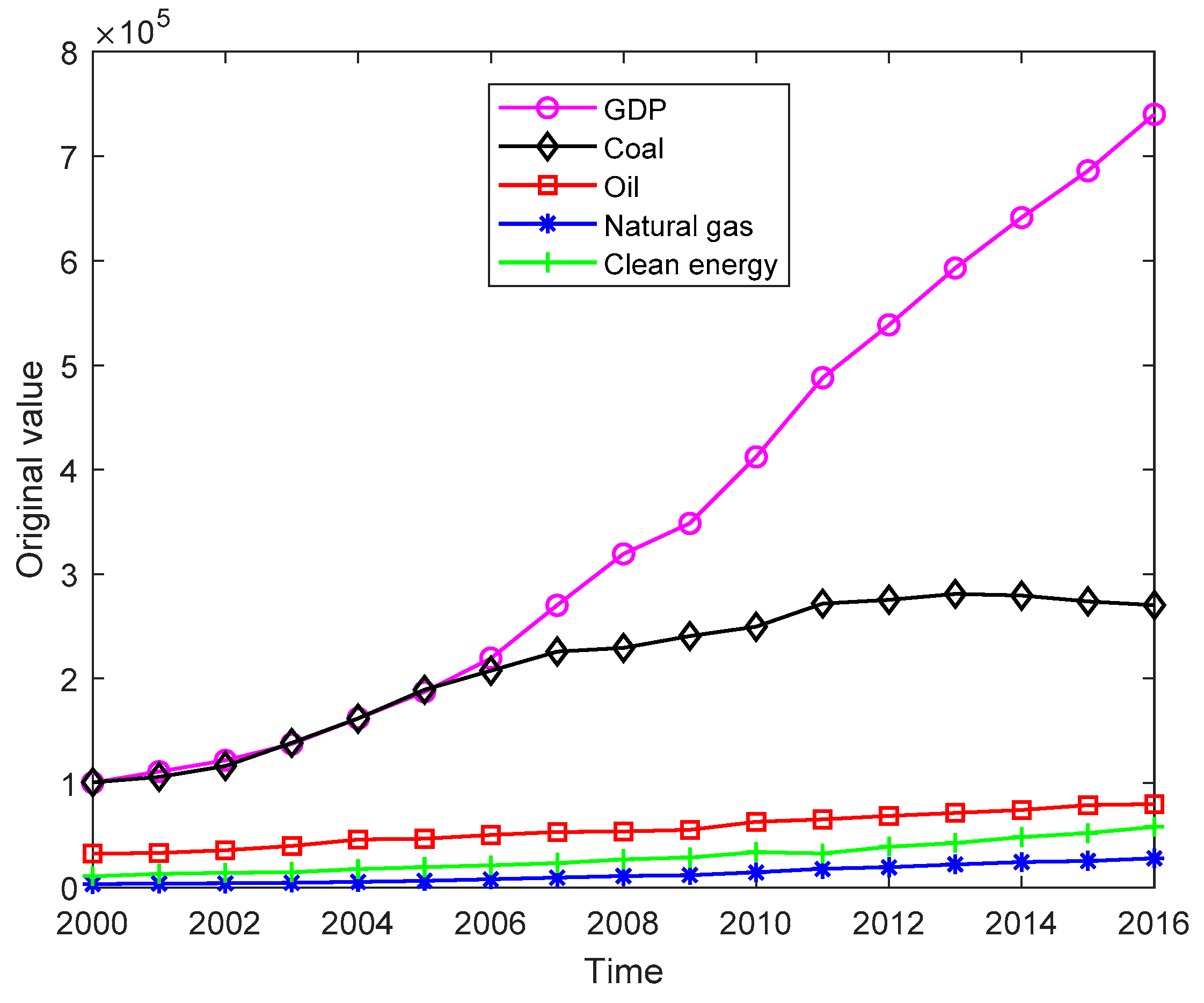
Figure 1 is the variation curves of China’s GDP and energy consumption. Figure 1 shows that GDP has the codirectional correlative influence relationships with C, O, G and R.

To find GDP’s correlative degrees with C, O, G and R, we calculate the correlative degrees below.

Table 2. GDP’s correlative coefficients with C, O, G and R.

Year	C	O	G	R
2000	0.6764	0.5716	0.9360	0.8220
2001	0.6829	0.5867	0.9570	0.7447
2002	0.6621	0.5724	0.9189	0.7469
2003	0.6020	0.5503	0.9305	0.7768
2004	0.5669	0.5193	0.9120	0.7317
2005	0.5237	0.5621	0.9222	0.7427
2006	0.5268	0.5825	0.9766	0.7804
2007	0.5680	0.6714	0.9395	0.8987
2008	0.6860	0.8524	0.9055	0.9297
2009	0.7207	0.9616	0.8767	0.9885
2010	0.9542	0.9460	0.9376	0.9765
2011	0.8215	0.6737	0.9458	0.6174
2012	0.6550	0.5925	1.0000	0.7058
2013	0.5431	0.5165	0.8623	0.6688
2014	0.4549	0.4656	0.8027	0.7387
2015	0.3884	0.4436	0.8722	0.7509
2016	0.3341	0.3874	0.7915	0.8348

shows GDP’s correlative coefficients with C, O, G and R.

In this way, we get the correlative degree between GDP and C, $r_C=0.6152$, the correlative degree between GDP and O, $r_O=0.6202$; the correlative degree between GDP and G, $r_G=0.9132$; the correlative degree between GDP and R, $r_R=0.7949$. Because $r_G>r_R>r_O>r_C$, G has the greatest influence on GDP, followed by R, O and C.

3.2. Multiplier Analysis Results

Here we make the multiplier analysis.

First, build a model

$$GDP=(1-{\lambda }_C)u_C+{\beta }_{C0}C+{\lambda }_{C}GDP\left(-1\right)$$

Because the correlation coefficient of independent variables $C$ and $GDP(-1)$, $r=0.8684$, close to 1, the two variables have the multicollinearity. To eliminate the multicollinearity, we use the principal component regression method proposed to build the model.

Because the contribution rate of principal component 1 is ${\alpha }_1=\frac{1.8684}{2}\times 100\%=93.42\%>90\%$, we choose principal component 1 for the regression, and then build the following model:

$$GDP=-203129.736311+1.805276\ast C+0.539583\ast GDP\left(-1\right)$$

The model’s coefficient of determination is $R^2=0.9593$.

It indicates the principal component regression model has the high fitting precision.

Then, build the model:

$$GDP=(1-{\lambda }_O)u_O+{\beta }_{O0}O+{\lambda }_{O}GDP\left(-1\right)$$

Because the correlation coefficient of independent variables $O$ and $GDP(-1)$, $r=0.9748$, close to 1, the two variables have the multicollinearity. To eliminate the multicollinearity, we use the principal component regression method proposed to build the model.

Because the contribution rate of principal component 1 is ${\alpha }_1=\frac{1.9748}{2}\times 100\%=98.74\%>90\%$, we choose principal component 1 for the regression, and then build the following model:

$$GDP=-217521.405045+7.233876\ast O+0.535354\ast GDP(-1)$$

The model’s coefficient of determination is $R^2=0.9944$.

It indicates the principal component regression model has the high fitting precision.

Then, build the model:

$$GDP=(1-{\lambda }_G)u_G+{\beta }_{G0}G+{\lambda }_{G}GDP\left(-1\right)$$

Because the correlation coefficient of independent variables $G$ and $GDP(-1)$, $r=0.9980$, close to 1, the two variables have the multicollinearity. To eliminate the multicollinearity, we use the principal component regression method proposed to build the model.

Because the contribution rate of principal component 1 is ${\alpha }_1=\frac{1.9980}{2}\times 100\%=99.90\%>90\%$, we choose principal component 1 for the regression, and then build the following model:

$$GDP=21673.126685+12.965336\ast G+0.533332\ast GDP(-1)$$

The model’s coefficient of determination is $R^2=0.9981$.

It indicates the principal component regression model has the high fitting precision.

Then, build the model:

$$GDP=(1-{\lambda }_R)u_R+{\beta }_{R0}G+{\lambda }_{R}GDP\left(-1\right).$$

Because the correlation coefficient of independent variables $R$ and $GDP(-1)$, $r=0.9928$, close to 1, the two variables have the multicollinearity. To eliminate the multicollinearity, we use the principal component regression method proposed to build the model.

Because the contribution rate of principal component 1 is ${\alpha }_1=\frac{1.9928}{2}\times 100\%=99.64\%>90\%$, we choose principal component 1 for the regression, and then build the following model:

$$GDP=-33213.241020+7.565750\ast R+0.532462\ast GDP(-1)$$

The model’s coefficient of determination is $R^2=0.9928$.

It indicates the principal component regression model has the high fitting precision.

Then, get coal (C)’s dynamic multiplier for economic growth (GDP)

$${\beta }_{Cj}=1.805276\times {0.539583}^j,(j=0,1,2,\cdot \cdot \cdot )$$

We get current multiplier ${\beta }_{C0}=1.805276$ and the dynamic multipliers of next two periods ${\beta }_{C1}=0.974096$ and ${\beta }_{C2}=0.525606$. And then, through calculation, we get $D_2=84.29\%$. We can see that GDP increases by ¥0.1805276 billion as current coal increases by 10,000 tons of standard coal. The influence of coal in lag period on GDP decreases year after year. In lag period 2, coal’s multiplier effect influence on GDP has reached 84.29%.

Coal’s long-term multiplier for GDP is

$${\beta }_C=\frac{{\beta }_{C0}}{1-{\lambda }_C}=3.920959$$

It shows in the long run, GDP increases by¥0.3920959 billion as coal increases by 10,000 tons of standard coal.

Oil (O)’s dynamic multiplier for economic growth (GDP) is

$${\beta }_{Oj}=7.233876\times {0.535354}^j,(j=0,1,2,\cdot \cdot \cdot )$$

We get current multiplier ${\beta }_{O0}=7.233876$ and the dynamic multipliers of next two periods ${\beta }_{O1}=\mathrm{0.3.872684}$ and ${\beta }_{C2}=2.073257$. And then, through calculation, we get $D_2=84.66\%$. We can see that GDP increases by 0.7233876 billion as current oil increases by 10,000 tons of standard coal. The influence of oil in lag period on GDP decreases year after year. In lag period 2, oil’s multiplier effect influence on GDP has reached 84.66%.

Oil’s long-term multiplier for GDP is

$${\beta }_O=\frac{{\beta }_{O0}}{1-{\lambda }_O}=15.568575$$

It shows in the long run GDP increases by ¥1.5568575 billion as oil increases by 10,000 tons of standard coal.

Natural gas (G)’s dynamic multiplier for economic growth (GDP) is

$${\beta }_{Gj}=12.965336\times {0.533332}^j,(j=0,1,2,\cdot \cdot \cdot )$$

We get current multiplier ${\beta }_{G0}=12.965336$ and the dynamic multipliers of next two periods ${\beta }_{G1}=6.914829$ and ${\beta }_{G2}=3.687899$. And then, through calculation, we get $D_2=84.83\%$. We can see that GDP increases by 1.2965336 billion as current natural gas increases by 10,000 tons of standard coal. The influence of natural gas in lag period on GDP decreases year after year. In lag period 2, natural gas’s multiplier effect influence on GDP has reached 84.83%.

Natural gas’s long-term multiplier for GDP is

$${\beta }_G=\frac{{\beta }_{G0}}{1-{\lambda }_G}=27.782783$$

It shows in the long run GDP increases by ¥2.778278 billion as oil increases by 10,000 tons of standard coal.

Clean energy (R)’s dynamic multiplier for economic growth (GDP) is

$${\beta }_{Rj}=7.565750\times {0.532462}^j,(j=0,1,2,\cdot \cdot \cdot )$$

We get current multiplier ${\beta }_{R0}=7.565750$ and the dynamic multipliers of next two periods ${\beta }_{R1}=4.028474$ and ${\beta }_{R2}=2.145010$. And then, through calculation, we get $D_2=84.90\%$. We can see that GDP increases by 0.7565750 billion as current clean energy increases by 10,000 tons of standard coal. The influence of clean energy in lag period on GDP decreases year after year. In lag period 2, clean energy’s multiplier effect influence on GDP has reached 84.90%.

Clean energy’s long-term multiplier for GDP is

$${\beta }_R=\frac{{\beta }_{R0}}{1-{\lambda }_R}=16.182107$$

It shows in the long run GDP increases by ¥1.6182107 billion as clean energy increases by 10,000 tons of standard coal.

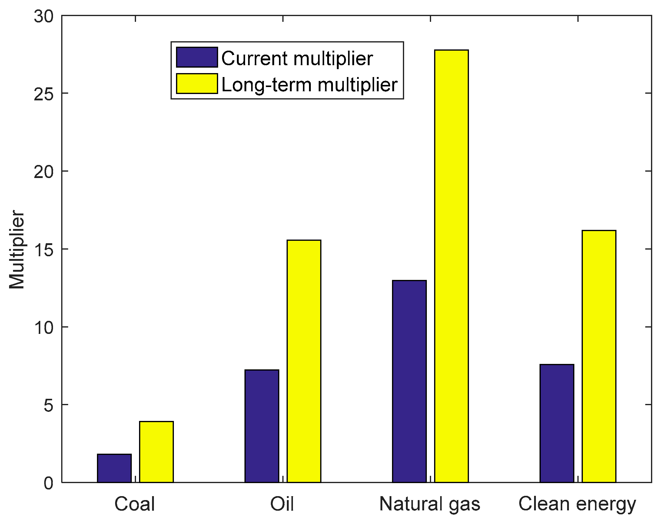
Figure 2 is the column diagram of multiplies of four types of energy. It shows that natural gas has the biggest current multiplier and long-term multiplier, followed by clean energy, oil and coal.

3.3. Contribution Rate Analysis Results

Here we calculate the contribution rates of fours energy consumption to economic growth.

Suppose the production function model is

$$\begin{array}{l}Y=A(t)K^{{\delta }_1}{L}^{{\delta }_2}{C}^{{\delta }_3}{O}^{{\delta }_4}{G}^{{\delta }_5}{R}^{{\delta }_6}\\ =A_0{e}^{\gamma t}{K}^{{\delta }_1}{L}^{{\delta }_2}{C}^{{\delta }_3}{O}^{{\delta }_4}{G}^{{\delta }_5}{R}^{{\delta }_6}\end{array}$$

where $A(t)=A_0{e}^{\gamma t}$ is technological progress level, K is the capital input, L is labor, (C, O, G, R) are energy input factors of coal, oil, natural gas and clean energy, Y is economic output which refers to GDP in the paper, and $(A_0,\gamma ,{\delta }_1,{\delta }_2,{\delta }_3,{\delta }_4,{\delta }_5,{\delta }_6)$ are parameters to be estimated.

The model is linearized to be

$$\ln GDP=\ln A_0+\gamma t+{\delta }_1\ln K+{\delta }_2\ln L+{\delta }_3\ln C+{\delta }_4\ln O+{\delta }_5\ln G+{\delta }_6\ln R$$

Through calculation, we get the following correlation coefficient matrix of independent variables $(t,\ln K,\ln L,\ln C,\ln O,\ln G,\ln R)$

$$\left(\begin{array}{l}1.0000 0.9955 0.9867 0.9260 0.9888 0.9949 0.9975\\ 0.9955 1.0000 0.9908 0.9506 0.9915 0.9983 0.9938\\ 0.9867 0.9908 1.0000 0.9685 0.9941 0.9868 0.9885\\ 0.9260 0.9506 0.9685 1.0000 0.9612 0.9440 0.9300\\ 0.9888 0.9915 0.9941 0.9612 1.0000 0.9890 0.9884\\ 0.9949 0.9983 0.9868 0.9440 0.9890 1.0000 0.9928\\ 0.9975 0.9938 0.9885 0.9300 0.9884 0.9928 1.0000\end{array}\right)$$

After calculation, get the characteristic roots

$$\left(\begin{array}{l}{\lambda }_1\\ {\lambda }_2\\ {\lambda }_3\\ {\lambda }_4\\ {\lambda }_5\\ {\lambda }_6\\ {\lambda }_7\end{array}\right)=\left(\begin{array}{l}6.8746\\ 0.1013\\ 0.0130\\ 0.0067\\ 0.0025\\ 0.0014\\ 0.0005\end{array}\right)$$

${\lambda }_1/{\lambda }_7=13749$ is very big, so there is the serious multicollinearity.

If using the method of OLS, the regression model built is

$$\begin{array}{l}\ln GDP=7.612973-0.018578t+0.286283\ln K-0.416560\ln L\\ -0.012379\ln C-0.011489\ln O+0.645759\mathrm{lnG}+0.069575\ln R\end{array}$$

Apparently, many variables’ coefficient signs are negative, which is unreasonable.

Because variables have the multicollinearity, the method of OLS is inapplicable, we use the nonlinear principal component regression method proposed to build the model.

Because the contribution rate of principal component 1 is ${\alpha }_1=\frac{6.8746}{7}\times 100\%=98.21\%>90\%$, we choose principal component 1 for the regression, and then build the following model

Through calculation, we get the regression coefficient

$$\begin{array}{l}(A_0,\gamma ,{\delta }_1,{\delta }_2,{\delta }_3,{\delta }_4,{\delta }_5,{\delta }_6) \\ =(e^{-48.449014},0.019593,0.099765,4.417489,0.265527,0.334042,0.134368,0.190468)\end{array}$$

i.e., the model built is

$$\begin{array}{l}\ln GDP=-48.449014+0.019593t+0.099765\ln K+4.417489\ln L\\ +0.265527\ln C+0.334042\ln O+0.134368\ln G+0.190468\ln R\end{array}$$

The model’s coefficient of determination $R^2=0.9999$.

We get the contribution rates of coal, oil, natural gas and clean energy to economic growth using the method given.

Table 3. Contribution rates of four energy consumption to economic growth.

Time	Coal	Oil	Natural Gas	Clean Energy
2001	0.0865	0.0434	0.1272	0.2473
2002	0.1875	0.1936	0.0444	0.0894
2003	0.2541	0.1947	0.1106	0.0497
2004	0.1875	0.2207	0.0949	0.1575
2005	0.2716	0.0328	0.1476	0.1237
2006	0.1566	0.1605	0.1811	0.1124
2007	0.1539	0.1245	0.1732	0.1261
2008	0.0357	0.0333	0.1844	0.2413
2009	0.1227	0.0924	0.0973	0.1069
2010	0.0603	0.2706	0.1713	0.2037
2011	0.1982	0.1043	0.2483	-0.0700
2012	0.0303	0.1390	0.0902	0.2883
2013	0.0495	0.1314	0.1703	0.1542
2014	-0.0164	0.1332	0.1307	0.2437
2015	-0.0694	0.2646	0.0782	0.1961
2016	-0.0488	0.0666	0.1816	0.2930

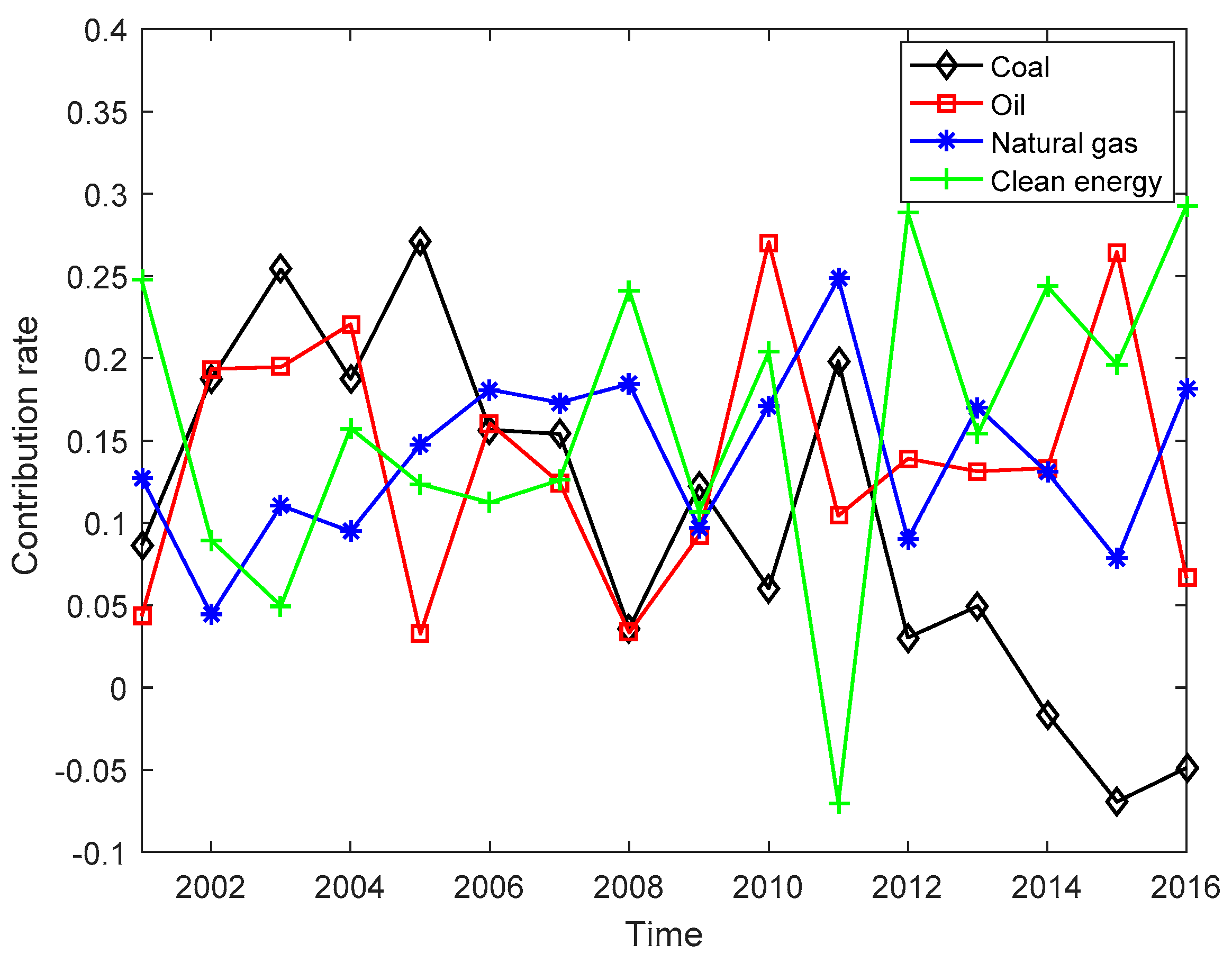
shows the results. Figure 3 is the variation diagram of contribution rates of four types of energy.

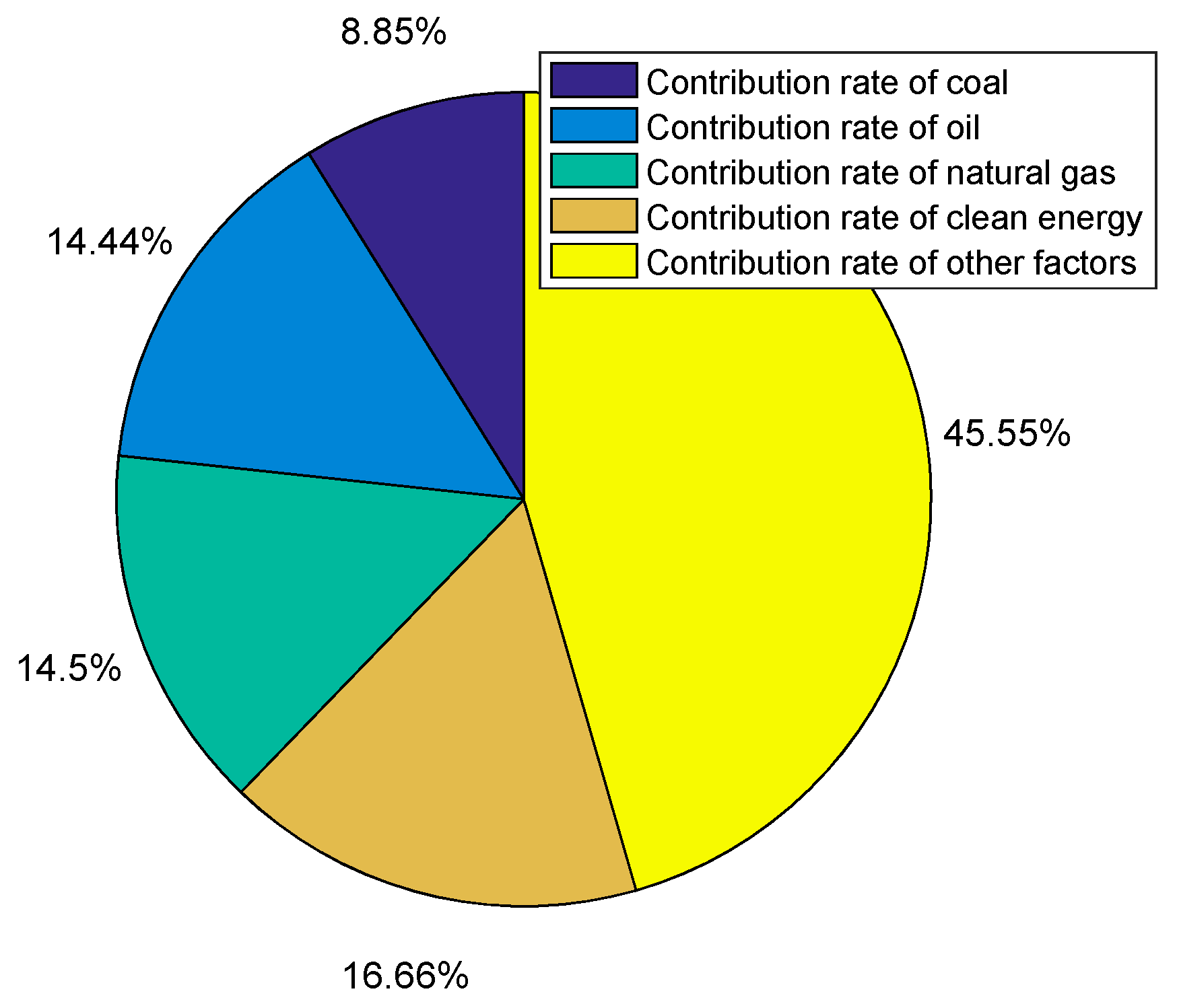
Table 3 and Figure 3 show that the economic growth in China mainly depends on clean energy, next on natural gas, oil and coal. The clean energy’s contribution rate presents a rising trend, while the coal’s contribution rate decreases. The average contribution rates of coal, oil, natural gas and clean energy were 8.85%, 14.44%, 14.50% and 16.66%, respectively, from year 2000 to year 2016, as shown in Figure 4.

4. Conclusions and Discussion

4.1. Main Conclusions

The paper makes a quantitative analysis on four energy consumption’s influences on economic growth from the following three aspects.

(1) The paper calculates the correlative degrees between four energy consumption and economic growth (GDP) to compare the influences of four energy consumption on economic growth in terms of correlative degree. Results show that the correlative degree between GDP and C is $r_C=0.6152$; the correlative degree between GDP and O is $r_O=0.6202$; the correlative degree between GDP and G is $r_G=0.9132$; the correlative degree between GDP and R is $r_R=0.7949$. Because $r_G>r_R>r_O>r_C$, natural gas has the greatest influence on GDP, followed by clean energy, oil and coal.

(2) The paper uses the dynamic linear regression model to calculate four energy consumption’s current multipliers, dynamic multipliers and long-term multipliers for economic growth, respectively, and compares the four energy consumption’s influences on economic growth in terms of marginal effect. Results show that coal, oil, natural gas and clean energy’s current multipliers are ${\beta }_{C0}=1.805276$, ${\beta }_{O0}=7.233876$, ${\beta }_{G0}=12.965336$ and ${\beta }_{R0}=7.565750$, respectively; their long-term multipliers are ${\beta }_C=3.920959$, ${\beta }_O=15.568575$, ${\beta }_G=27.782783$ and ${\beta }_R=16.182107$, respectively. We can see that natural gas has the greatest current multiplier, followed by clean energy, oil and coal. Natural gas also has the greatest long-term multiplier, followed by clean energy, oil and coal.

(3) The paper uses the production function model to calculate the contribution rates of four kinds of energy consumption to economic growth and then compares four energy consumption’s influences on economic growth in terms of input and output. Results show that the contribution rates of coal, oil, natural gas and clean energy consumption were 8.85%, 14.44%, 14.50% and 16.66%, respectively, from 2000 to 2016. We can see that clean energy has the greatest contribution rate to economic growth, followed by natural gas, oil and coal. The variation process shows that clean energy’s contribution rate has a rising trend while coal’s contribution rate declines; the contribution rates of oil and natural gas show few changes.

4.2. Discussion

Many researchers have analyzed the relationship between energy consumption and economic growth, but the paper analyzes the influences of different energy consumption on economic growth quantitatively in China. The paper first calculates the degrees of correlations between four energy consumption and economic growth (GDP). In terms of correlation, China’s natural gas consumption has the greatest correlation degree with GDP (0.9132), followed by clean energy (0.7949), oil (0.6202) and coal (0.6152). It indicates that natural gas consumption has a significant influence on GDP in China, with a correlation degree exceeding 0.9; clean energy also has a great influence on GDP, showing a correlation degree of near 0.8; oil and coal show comparatively smaller correlation degrees which also exceed 0.6, indicating they also have certain influences on economic growth. Next, the paper uses a lagged variable regression model to calculate four energy consumption’s multipliers to economic growth. In terms of marginal effect, in China, natural gas has the biggest current multiplier (12.965336), followed by clean energy (7.565750), oil (7.233876) and coal (1.805276); natural gas has the biggest long-term multiplier (27.782783), followed by clean energy (16.182107), oil (15.568575) and coal (3.920959). Therefore, from the perspective of marginal effect, in China, natural gas consumption has the greatest influence on GDP and its multiplier is also big; clean energy and oil consumption has similar influences on economic growth and pretty big multipliers; coal has a smaller influence on economic growth and smaller multipliers. It should be noticed that natural gas and clean energy has big multiplies, but, with small cardinal numbers, their influences are limited, while coal, although with small multiplies, has a big cardinal number, and thus has certain influence on economy. Finally, the paper uses the production function model to calculate four energy consumption’s contribution rates to economic growth. Input and output data show that, clean energy had the biggest average contribution rate (16.66%) from 2000 to 2016, followed by natural gas (14.50%), oil (14.44%) and coal (8.85%). It is clear that clean energy has the biggest contribution rate to economic growth; natural gas and oil also have great contribution rates to economic growth; coal has a comparatively smaller contribution rate, which also exceeds 8%, to economic growth. In terms of changing process, clean energy’s contribution rate shows a rising trend; coal’s contribution rate declines; for oil and natural gas, their contribution rates do not change a lot. From the analysis results of three methods we can see that the high-quality energy has the greatest influence on China’s economy. To realize the sustainable and stable growth of economy, China should increase the proportions of clean energy and natural gas consumption and reduce the proportion of coal consumption. Besides, the results indicate that China’s economy is developing in the direction of a green economy.

5. Recommendations

China’s energy development strategy in the low carbon economy pattern in the future should be improving the efficiency of energy utilization and optimizing the structure of energy use to ensure friendly environment and sustainably economic development.

First, China should improve the efficiency of energy utilization. Our research shows that China’s natural gas consumption and clean energy consumption has greater influences on economic growth than coal consumption and oil consumption, but coal consumption and oil consumption also has great influences on economic growth, especially oil consumption. In China, the consumption of traditional energy, such as coal and oil, still plays an important role in economic growth. Therefore, the urgent task on hand of China’s economic growth is sticking to the energy-saving, cost-reducing and pollution-deceasing way, encouraging the research and development of energy-saving and cost-reducing technologies, increasing the input in energy technology innovation and enhancing the utilization ratio of traditional energy like coal and oil continuously to realize the high-efficient utilization of traditional energy. To emphasize the comprehensive, coordinated and sustainable development and seek the unification of economic, social and ecological benefits, China should focus on the following two aspects. On the one hand, China should use existing energy-saving technologies and new technologies to improve energy-consumption equipment to make each unit of energy play its role fully, such as improving the drive efficiency of motor, installing heating and refrigerating systems with better energy efficiency and so on. On the other hand, the government should develop people’s consciousness of energy conservation, change enterprises’ production patterns through legal encouragement and supervision, such as improving energy efficiency standards for enterprises, establishing incentive mechanisms and introducing the market pressure to enhance state-owned enterprises’ performance.

Next, China should optimize energy utilization structure. Although in China natural gas consumption and clean energy consumption have greater influences on economic growth than coal consumption and oil consumption, their proportions are smaller than coal and oil, so China need to improve the unreasonable energy consumption structure, reduce the proportions of traditional energy like coal and oil in energy consumption gradually, increase the proportion of clean energy actively and try to change the extensive economic growth pattern currently in China into the intensive growth pattern. China should make efforts from the following two aspects. On the one hand, China should gather the aggregate risk diversification capacity of insurance market, monetary market and capital market by designing financial derivatives of carbon, such as low carbon (LC) credit, LC bond funds, LC trust, LC insurance and so on, devote major efforts to developing the industry of renewable energy resources and new-type energy industry, adjust energy consumption’s layout structure and supply-demand structure, and promote the healthy and sustainable development of China’s energy industry. On the other hand, China should use policies to guide and support the diversification of energy consumption structure and encourage the development and utilization of new energy and renewable energy continuously. Developing new-type and renewable energy, such as hydroenergy, nuclear energy and wind energy, is the new tend of China’s energy consumption in the future, and also an important approach to replace traditional energy consumption and solve China’s problem of high-energy-consumption economic growth.

Finally, China should plan and develop energy development strategies. Under the new situation of reform and development of China, energy’s influence on economic growth will be increasingly great. Therefore, China should recognize and deal with the relationship between energy consumption and economic growth properly, and reform the traditional energy development mode. The government of China should develop a reasonable energy development plan consistent with China’s economic development situation by taking current problems, such as the poor energy resources per capita, the high energy consumption intensity, the unreasonable energy structure and so on, in to consideration while developing the overall economic development strategy.

References

1. Kraft, J.; Kraft, A. On the relationship between energy and GNP. J. Energy Dev. 1978, 3, 401–403. [Google Scholar]
2. Yu, E.S.H.; Jin, J.C. Cointegration tests of energy consumption, income, and employment. Resour. Energy 1992, 14, 259–266. [Google Scholar] [CrossRef]
3. Stern, D.I. Energy and economic growth in the USA: A multivariate approach. Energy Econ. 1993, 15, 137–150. [Google Scholar] [CrossRef]
4. Stern, D.I. A multivariate cointegration analysis of the role of energy in the US macroeconomy. Energy Econ. 2000, 22, 267–283. [Google Scholar] [CrossRef] [Green Version]
5. Oh, W.; Lee, K. Causal relationship between energy consumption and GDP revisited: The case of Korea 1970–1999. Energy Econ. 2004, 26, 51–59. [Google Scholar] [CrossRef]
6. Paul, S.; Bhattacharya, R.N. Causality between energy consumption and economic growth in India:a note on conflicting results. Energy Econ. 2004, 26, 977–983. [Google Scholar] [CrossRef]
7. Zamani, M. Energy consumption and economic activities in Iran. Energy Econ. 2007, 29, 1135–1140. [Google Scholar] [CrossRef]
8. Van Montfort, C.A.G.M.; Lise, W. Energy consumption and GDP in Turkey: Is there a cointegration relationship. Energy Econ. 2007, 29, 1166–1178. [Google Scholar]
9. Chen, S.W.; Xie, Z.X.; Liao, Y. Energy consumption promotes economic growth or economic growth causes energy use in China? A panel data analysis. Empir. Econ. 2018, 55, 1019–1043. [Google Scholar] [CrossRef]
10. Appiah, M.O. Investigating the multivariate Granger causality between energy consumption, economic growth and CO2 emissions in Ghana. Energy Policy 2018, 112, 198–208. [Google Scholar] [CrossRef]
11. Tang, C.F.; Tan, B.W.; Ozturk, I. Energy consumption and economic growth in Vietnam. Renew. Sustain. Energy Rev. 2016, 54, 1506–1514. [Google Scholar] [CrossRef]
12. Gorus, M.S.; Aydin, M. The relationship between energy consumption, economic growth, and CO2 emission in MENA countries: Causality analysis in the frequency domain. Energy 2019, 168, 815–822. [Google Scholar] [CrossRef]
13. Murad, M.W.; Alam, M.M.; Noman, A.H.M.; Ozturk, I. Dynamics of technological innovation, energy consumption, energy price and economic growth in Denmark. Environ. Prog. Sustain. Energy 2019, 38, 22–29. [Google Scholar] [CrossRef]
14. Latief, R.; Lefen, L. Foreign Direct Investment in the Power and Energy Sector, Energy Consumption, and Economic Growth: Empirical Evidence from Pakistan. Sustainability 2019, 11, 192. [Google Scholar] [CrossRef]
15. Sanu, S.; Ahmad, F. The Linkage between Energy Consumption and Economic Growth in India: Evidence Based on Cointegration and Error Correction Modelling Techniques. Asian J. Res. Soc. Sci. Hum. 2017, 7, 250–260. [Google Scholar] [CrossRef]
16. Liu, X. Aggregate and disaggregate analysis on energy consumption and economic growth nexus in China. Environ. Sci. Pollut. Res. 2018, 25, 26512–26526. [Google Scholar] [CrossRef]
17. Lin, B.Q.; Moubarak, M. Renewable energy consumption–Economic growth nexus for China. Renew. Sustain. Energy Rev. 2014, 40, 111–117. [Google Scholar] [CrossRef]
18. Ouyang, Y.F.; Li, P. On the nexus of financial development, economic growth, and energy consumption in China: New perspective from a GMM panel VAR approach. Energy Econ. 2018, 71, 238–252. [Google Scholar] [CrossRef]
19. Ohlan, R. Renewable and nonrenewable energy consumption and economic growth in India. Energy Source Part B 2016, 11, 1050–1054. [Google Scholar] [CrossRef]
20. Dai, H.C.; Xie, X.X.; Xie, Y.; Liu, J.; Masui, T. Green growth: The economic impacts of large-scale renewable energy development. Appl. Energy 2016, 162, 435–449. [Google Scholar] [CrossRef]
21. Rahman, M.M.; Mamun, S.A.K. Energy use, international trade and economic growth nexus in Australia: New evidence from an extended growth model. Renew. Sustain. Energy Rev. 2016, 64, 806–816. [Google Scholar] [CrossRef]
22. Dogan, E. Analyzing the linkage between renewable and non-renewable energy consumption and economic growth by considering structural break in time-series data. Renew. Energy 2016, 99, 1126–1136. [Google Scholar] [CrossRef]
23. Raza, S.A.; Shah, N.; Sharif, A. Time frequency relationship between energy consumption, economic growth and environmental degradation in the United States: Evidence from transportation sector. Energy 2019, 173, 706–720. [Google Scholar] [CrossRef]
24. Ahmad, M.; Zhao, Z.Y.; Li, H. Revealing stylized empirical interactions among construction sector, urbanization, energy consumption, economic growth and CO2 emissions in China. Sci. Total Environ. 2019, 657, 1085–1098. [Google Scholar] [CrossRef] [PubMed]
25. Chiou-Wei, S.Z.; Zhu, Z.; Chen, S.H.; Hsueh, S.P. Controlling for relevant variables: Energy consumption and economic growth nexus revisited in an EGARCH-M (Exponential GARCH-in-Mean) model. Energy 2016, 109, 391–399. [Google Scholar] [CrossRef]
26. Ntanos, S.; Skordoulis, M.; Kyriakopoulos, G.; Arabatzis, G.; Chalikias, M.; Galatsidas, S.; Batzios, A.; Katsarou, A. Renewable energy and economic growth: Evidence from European countries. Sustainability 2018, 10, 2626. [Google Scholar] [CrossRef]
27. Jabeur, S.B.; Sghaier, A. The relationship between energy, pollution, economic growth and corruption: A Partial Least Squares Structural Equation Modeling (PLS-SEM) approach. Econ. Bull. 2018, 38, 1927–1946. [Google Scholar]
28. Nasreen, S.; Saidi, S.; Ozturk, I. Assessing links between energy consumption, freight transport, and economic growth: Evidence from dynamic simultaneous equation models. Env. Sci. Pollut. Res. 2018, 25, 16825–16841. [Google Scholar] [CrossRef]
29. Lin, B.; Nelson, B.I. Causal relationships between energy consumption, foreign direct investment and economic growth for MINT: Evidence from panel dynamic ordinary least square models. J. Clean. Prod. 2018, 197, 708–720. [Google Scholar] [CrossRef]
30. Haseeb, M.; Hassan, S.; Azam, M. Rural-urban transformation, energy consumption, economic growth, and CO2 emissions using STRIPAT model for BRICS countries. Environ. Prog. Sustain. Energy 2017, 36, 523–531. [Google Scholar] [CrossRef]
31. Adewuyi, A.O.; Awodumi, O.B. Biomass energy consumption, economic growth and carbon emissions: Fresh evidence from West Africa using a simultaneous equation model. Energy 2017, 119, 453–471. [Google Scholar] [CrossRef]
32. Li, B.J.; Wang, T.H.; Meng, F.L. Double Quantitative Analysis of the Effects of Meteorological Factors on Winter Wheat Yield at Different Growth Stages Based on Grey Relational Analysis. J. Grey Syst. 2018, 30, 31–43. [Google Scholar]
33. Chang, S.; Huang, F.; Zhao, J.J. Identifying Influential Climate Factors of Land Surface Phenology Changes in Songnen Plain of China Using Grid-based Grey Relational Analysis. J. Grey Syst. 2018, 30, 18–33. [Google Scholar]
34. Es, H.A.; Hamzacebi, C.; Firat, S.U.O. GRA-TRI: A Multicriteria Decision Aid Classification Method based on Grey Relational Analysis. J. Grey Syst. 2018, 30, 1–12. [Google Scholar]
35. Balaji, S.; Sakthivel, M.; Pasupathy, S.A.; Karthick Kumar, K.; Sukanya, G. Multi Objective Optimization of Anaerobic Digestion of Poultry Litter Using Taguchi Grey Relational Analysis. Int. J. Appl. Eng. Res. 2018, 13 (Pt. 4), 5216–5222. [Google Scholar]
36. Yang, L.; Xie, N.M. Evaluation of provincial integration degree of “internet plus industry” based on matrix grey relational analysis Case of China 2014–2016. Grey Syst. Theory. App. 2019, 9, 31–44. [Google Scholar] [CrossRef]
37. Satolo, E.G.; Leite, C.; Calado, R.D. Ranking lean tools for world class reach through grey relational analysis. Grey Syst. Theory. Appl. 2018, 8, 399–423. [Google Scholar] [CrossRef] [Green Version]
38. Bildirici, M.E.; Bakirtas, T.; Kayikci, F. Economic growth and electricity consumption: Auto regressive distributed lag analysis. J. Energy S. Afr. 2017, 23, 29–45. [Google Scholar] [CrossRef]
39. Matthew, O.; Osabohien, R.; Fagbeminiyi, F.; Fasina, A. Greenhouse Gas Emissions and Health Outcomes in Nigeria: Empirical Insight from Auto-regressive Distribution Lag Technique. Int. J. Energy Econ. Policy 2018, 8, 43–50. [Google Scholar]
40. Akpansung, A.O.; Waziri, S.E. Has Financial Liberalisation Promoted Economic Growth in Nigeria? Evidence from Auto-Regressive Distributed Lag (ARDL) Approach. Asian Econ. Financ. Rev. 2018, 8, 172–188. [Google Scholar] [CrossRef] [Green Version]
41. Phiri, M.; Shiferaw, Y.A.; Tesfamichael, S.G. Modelling the relationship between groundwater depth and NDVI using time series regression with Distributed Lag Models. S. Afr. J. Geomat. 2018, 7, 147–163. [Google Scholar] [CrossRef]
42. He, Y.; Gao, S.W.; Liao, N. An intelligent computing approach to evaluating the contribution rate of talent on economic growth. Comput. Econ. 2016, 48, 399–423. [Google Scholar] [CrossRef]
43. Guo, H.; Hu, J.; Yu, S.; Sun, H.; Chen, Y. Computing of the contribution rate of scientific and technological progress to economic growth in Chinese regions. Expert Syst. Appl. 2012, 39, 8514–8521. [Google Scholar] [CrossRef]
44. Zhao, C.G.; Xu, Y.L.; Feng, Y.J. A study on contribution rate of management elements in economic growth. Comput. Intell. Syst. 2011, 234, 151–158. [Google Scholar]
45. Cheng, M.L. A Grey CES Production Function Model and Its Application in Calculating the Contribution Rate of Economic Growth Factors. Complexity 2019, 2019, 5617061. [Google Scholar] [CrossRef]
46. Cheng, M.L.; Shi, G.J.; Han, Y. A Modified CES Production Function Model and Its Application in Calculating the Contribution Rate of Energy and Other Influencing Factors to Economic Growth. J. Syst. Sci. Inf. 2019, 7, 161–172. [Google Scholar] [CrossRef]
47. Tucker, J.D.; Lewis, J.R.; Srivastava, A. Elastic functional principal component regression. Stat. Anal. Data Min. 2019, 12, 101–115. [Google Scholar] [CrossRef]
48. Li, Y.L.; Yang, H. Performance of the restricted almost unbiased type principal components estimators in linear regression model. Stat. Pap. 2019, 60, 19–34. [Google Scholar] [CrossRef]
49. Li, Y.H.; Zhang, Y.; Liu, T.Y. Analysis of principal component regression equations of air transportation and local economy: Taking tianjin as an example. Theor. Econ. Lett. 2018, 8, 1830–1839. [Google Scholar] [CrossRef]
50. Kasemsiri, P.; Dulsang, N.; Pongsa, U.; Hiziroglu, S.; Chindaprasirt, P. Optimization of Biodegradable Foam Composites from Cassava Starch, Oil Palm Fiber, Chitosan and Palm Oil Using Taguchi Method and Grey Relational Analysis. J. Polym. Environ. 2017, 25, 378–390. [Google Scholar] [CrossRef]
51. Jiang, H.; Lin, J.Y.; Jiang, P. Using Grey Relational Analysis with Entropy to Predict the International Financial Center of China. J. Syst. Sci. Inf. 2017, 5, 88–96. [Google Scholar] [CrossRef]
52. Han, M.; Zhang, R.Q.; Xu, M.L. A variable selection algorithm based on improved grey relational analysis. Control Decis. 2017, 32, 1647–1652. [Google Scholar]
53. Jin, X.; Yin, K.D.; Li, X.M. Grey relational analysis on the land-sea economy in China. Grey Syst. Theory. Appl. 2017, 7, 31–44. [Google Scholar] [CrossRef]
54. Kuo, T. A Review of Some Modified Grey Relational Analysis Models. J. Grey Syst. 2017, 29, 70–77. [Google Scholar]
55. Gasparrini, A. Modeling exposure–lag–response associations with distributed lag non-linear models. Stat. Med. 2014, 33, 881–899. [Google Scholar] [CrossRef] [PubMed]
56. Mahmood, H.; Alkhateeb, T.T.Y. Testing Asymmetrical Effect of Exchange Rate on Saudi Service Sector Trade: A Non-linear Auto-regressive Distributive Lag Approach. Int. J. Econ. Financ. I 2017, 7, 73–77. [Google Scholar]
57. Miller, J.I. Mixed-frequency Cointegrating Regressions with Parsimonious Distributed Lag Structures. J. Financ. Econ. 2014, 12, 584–614. [Google Scholar] [CrossRef]
58. Seposo, X.T.; Dang, T.N.; Honda, Y. Evaluating the Effects of Temperature on Mortality in Manila City (Philippines) from 2006–2010 Using a Distributed Lag Nonlinear Model. Int. J Environ. Res. Public Health 2015, 12, 6842–6857. [Google Scholar] [CrossRef]
59. Muggeo, V.M.R. Analyzing temperature effects on mortality within the R environment: The constrained segmented distributed lag parameterization. J. Stat. Softw. 2010, 32, 1–17. [Google Scholar] [CrossRef]
60. Li, X.Y. The Variation Tendency Analysis on Contribution Rate to Economic Growth by Production Factor Input in China. Manag. Sci. Eng. 2013, 7, 16–23. [Google Scholar] [CrossRef]
61. Zhu, K.; Guo, H.; Diao, F.; Xu, S. A better estimate to the contribution rate of education on economic growth in China from 1999 to 2003. Expert Syst. Appl. 2008, 34, 1371–1383. [Google Scholar] [CrossRef]
62. Hu, J.Y.; Gao, Z.J. Re-estimation the Contribution Rate of Technological Progress to Economic Growth Accounting for Energy Consumption Factors Based on Time Series Data of China (1991–2011). J. Appl. Sci. 2013, 13, 2346–2350. [Google Scholar]
63. Sun, H.; Guo, H.; Hu, J.; Zhu, K. Comparative study on economic contribution rate of education of China and foreign countries based on soft computing method. Appl. Soft Comput. 2012, 12, 2106–2113. [Google Scholar] [CrossRef]
64. He, Y.; Liao, N.; Liu, H.; Zhong, Y. A new method of soft computing to estimate the contribution rate of S&T progress on economic growth. Appl. Soft Comput. 2012, 12, 1801–1809. [Google Scholar]
Figure 1. Variation curves of China’s economic growth (GDP) and energy consumption.
Sustainability 11 03982 g001
Figure 2. The column diagram of multipliers of four energies.
Sustainability 11 03982 g002
Figure 3. The variation diagram of contribution rates of four energy consumption.
Sustainability 11 03982 g003
Figure 4. Contribution rates of four energies.
Sustainability 11 03982 g004