Assessing Impacts of Climate Variability and Reforestation Activities on Water Resources in the Headwaters of the Segura River Basin (SE Spain)

Abstract

Climate change and the land-use and land-cover changes (LULC) resulting from anthropic activity are important factors in the degradation of an ecosystem and in the availability of a basin’s water resources. To know how these activities affect the quantity of the water resources of basins, such as the Segura River Basin, is of vital importance. In this work, the Soil and Water Assessment Tool (SWAT) was used for the study of the abovementioned impacts. The model was validated by obtaining a Nash–Sutcliffe efficiency (NSE) of 0.88 and a percent bias (PBIAS) of 17.23%, indicating that SWAT accurately replicated monthly streamflow. Next, land-use maps for the years of 1956 and 2007 were used to establish a series of scenarios that allowed us to evaluate the effects of these activities on both joint and individual water resources. A reforestation plan applied in the basin during the 1970s caused that the forest area had almost doubled, whereas the agricultural areas and shrubland had been reduced by one-third. These modifications, together with the effect of climate change, have led to a decrease of 26.3% in the quantity of generated water resources, not only due to climate change but also due to the increase in forest area.

1. Introduction

Water resources have suffered an important decrease in recent decades due to the effects of human activities and climate change [1]. This is especially the case in semi-arid regions, where water resources have become a critical element of socioeconomic development [2]. Many recent studies have studied the driving factors of the hydrological cycle, reaching the conclusion that climate and land-use/land-cover changes (LULC) are two critical factors that affect the hydrological processes in the basin [3]. On the one hand, climate change projections during this century in the Mediterranean region reveal a rise in temperature accompanied by a decrease in precipitation, resulting in a decrease of the water resources by over 20% [4]. In fact, recent studies in the headwaters of the Segura River Basin (HWSRB) [5] predicted a decrease of over 50% by the end of the century. Furthermore, human activities such as agricultural irrigation expansion or urbanization affect the availability of water resources through their influence on runoff. This is especially true in Mediterranean Europe, where human activities have modified the landscape [6,7,8]. Developing a better understanding of the influence of LULC on the hydrological processes of a watershed is essential for sustainable water resource management. This is particularly true in the Segura River Basin, which is located in a semi-arid region of southeast Spain, and where we can find the most water-stressed basin in Western Europe [9]. The HWSRB are relevant due to its 9% water resource contribution, in spite of the fact that it covers only 1.2% of the area over the total watershed [5].

The use of a physically based distributed hydrological model is a common approach to evaluating the impact of LULC changes on water resources [10]. From the hydrological models available, we chose the Soil and Water Assessment Tool (SWAT) model due to the fact that this model has been used worldwide to simulate the hydrological cycle and has been used extensively to evaluate the impacts of LULC changes on watershed hydrology [11]. Likewise, a multitude of studies have addressed separating the influences of human activities and climate variability on water resources using the SWAT model [3,11,12,13]. However, only two references have been found on the application of the SWAT model to assess the impacts of LULC changes in Spain. Molina-Navarro et al. [14] analyzed the potential effects of climate change and land-use management scenarios on water discharge and the water quality of the Pareja Reservoir located in the upper Tagus River Basin. Salmoral et al. [15] assessed the water-related impacts of land-use changes and agricultural practices, combining the use of the SWAT model and a water footprint assessment in the Genil River Basin (southern Spain).

Significant LULC have occurred in the southeastern part of Spain since the 1970s as a result of the progressive abandonment of dryland agricultural activities and the implementation of reforestation plans increasing forest cover [16]. The strategy for reforesting the HWSRB was to introduce pine species; pinus nigra was used in upper parts of the basin, whereas pinus pinaster and pinus halepensis were used in the intermediate and lower parts of the basin [17]. This increase of vegetation cover leads not only to a decrease in sediment yield [18] but also to a decrease in runoff generation. Several studies have analysed the potential water yield reduction due to forestation activities. Bosch and Hewlett [19] studied the effect of vegetation changes on the water yield on 94 different basins. They concluded that eucalypt and pine forest types cause a reduction of 40 mm in water yield per 10% change in cover, but in the case of shrubland, this reduction is four times lower (10 mm). Other authors added new basins in addition to those reviewed by Bosch and Hewlett; for example, Sahin and Hall [20] analysed 145 basins using a fuzzy linear regression analysis reaching similar conclusions, whereas Brown et al. [21] reviewed 166 basins focusing not only on water yield but also on low flows. Sun et al. [22] analysed the potential magnitude of annual water yield to forestation across China, suggesting that this reduction can vary from 30% in tropical regions to 50% in semiarid regions. Llorens et al. [23] studied a Mediterranean mountain basin showing a reduction in runoff up to 18% due to the reforestation activities using pine trees.

Due to the high water stress suffered in the Segura River Basin, the impact of forest restoration on water yield must be evaluated. Therefore, the objectives of this study were as follows: (1) to determine trends in the annual and monthly precipitation and temperature; (2) to calibrate and validate the SWAT model in a data-scarce river basin with a Mediterranean climate, such as the HWSRB; and (3) to analyze the impact of climate variability and reforestation activities on runoff and evapotranspiration (ET).

2. Materials and Methods

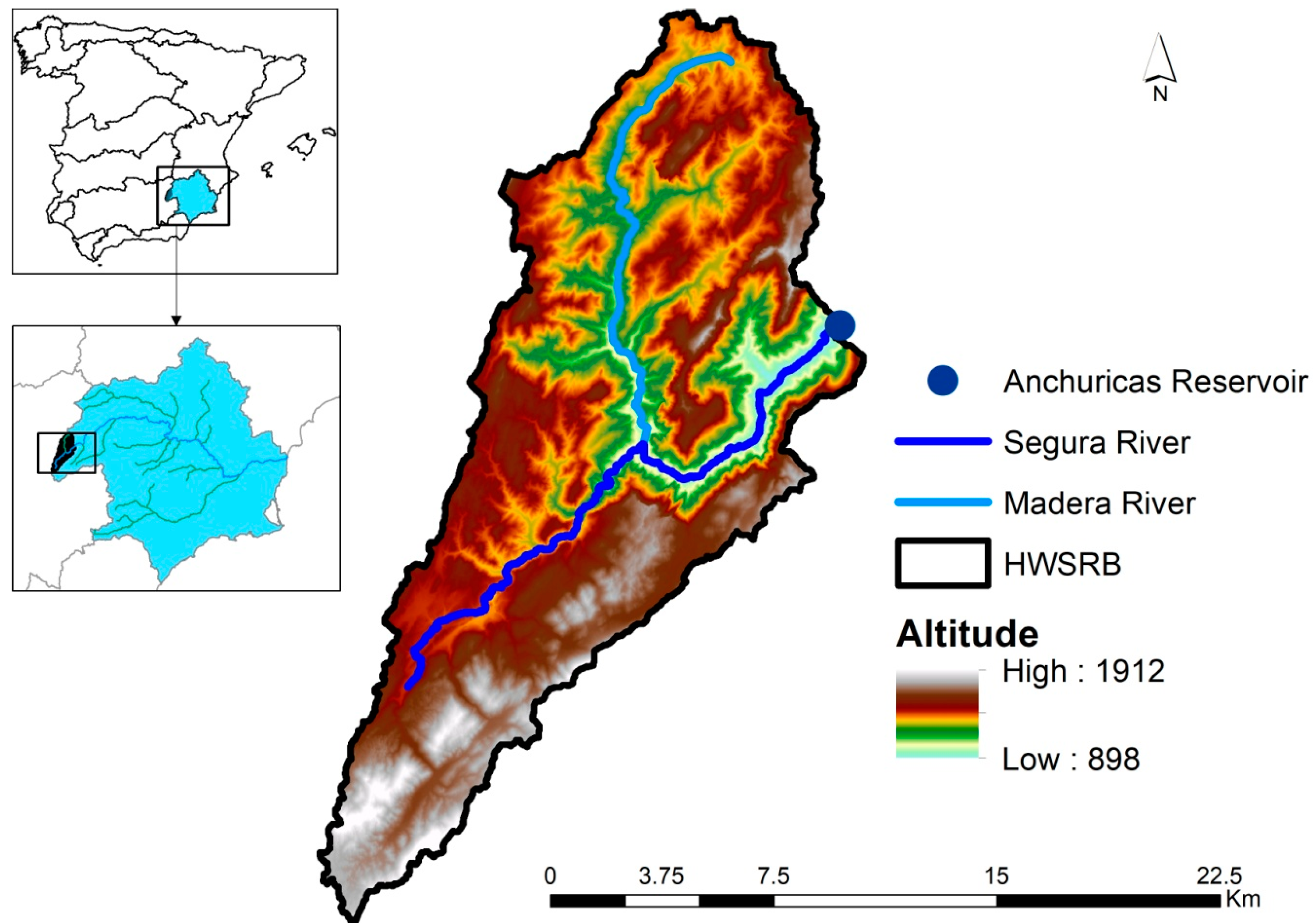
2.1. Study Area Description

The Segura River Basin represents one of the most arid zones of the Mediterranean area, presenting great heterogeneity in its flow regimes [24]. It is located in the southeastern part of Spain (Figure 1). The SWAT model was applied to the 235 km² of the HWSRB that flow into the Anchuricas Reservoir, which has a capacity of 6 hm³ and exists to generate electricity. As the terrain is mountainous, it presents steep slopes with an elevation range from 898 to 1912 m. According to data from 1951 to 2015, the average annual precipitation is above 800 mm, ranging from 381 mm to 1447 mm. As a typical Mediterranean climate, precipitation is received mainly during spring and autumn while it is insignificant during summer. The average annual temperature was 11.8 °C.

The mean monthly flow of this river leaving the mountains varies between 0.74 m³/s in August to 4.82 m³/s in February. Land cover in the watershed is mostly a forest-dominated area and features Mediterranean shrubland vegetation, which covers about 81% of the basin. The rest of the land is mainly used for range purposes. The main soil type is Rendzic Leptosol, which presents a variable depth but always less than 50 cm, abundant stoniness, high carbon levels and good drainage [5]. The study area is characterized by the fundamental role of the groundwater in the surface hydrology due to the fact that a significant part of the streamflow comes from groundwater sources. The large volume of precipitations and the abundance of outcropping carbonate rocks have caused the formation of karstic systems [25].

2.2. The Precipitation and Temperature Trend Analysis

In this study, Microsoft Excel template application MAKESENS (Version 1.0) was used to calculate the trends and changing rates of temperature and precipitation. This application includes the non-parametric Mann–Kendall (MK) test for the trend and Sen’s non-parametric method for the magnitude of the trend. More details regarding the MAKESENS model can be found in Salmi et al. [26]. The MK test was used to detect the change in the annual and monthly temperature and precipitation. The advantage of the MK test, which is one of the most widely used nonparametric tests for detecting trends in hydroclimatic series [27], is that it does not require the data to be distributed normally and it has a low sensitivity to abrupt peaks due to inhomogeneous time series [28]. The complete description and formulae of the MK test can be obtained from Partal and Kahya [29]. The magnitudes of the estimated changes in the trend of temperature and precipitation were estimated by using a simple non-parametric procedure that Sen developed. The Sen [30] method alleviates the consequences of anomalous trends by using the median of the series of slopes as the judgmental foundation [13]. The $Q_i$ is given by the following:

$$Q_i=median\left(\frac{x_j-x_k}{j-k}\right)\forall k\le j$$

(1)

where $x_j$ and $x_k$ are data values at times j and k, respectively. Estimator $Q_i$ is the median over all combinations of record pairs for the entire dataset. A positive slope magnitude indicates an increasing tendency, whereas a negative slope magnitude indicates a decreasing tendency in the time series.

2.3. Description of SWAT Model

Hydrological modeling was performed using the SWAT extension for the QGIS interface, called QSWAT [31]. SWAT is a continuous-time, long-term, semi-distributed and physically based model. SWAT considers the heterogeneity of a watershed by dividing it into multiple sub-watersheds based on the river network and topography; subsequently, sub-watersheds are divided into hydrologic response units (HRUs) consisting of homogeneous land use, land management, and soil characteristics. These HRUs represent percentages of the sub-watershed area and are not identified spatially within a SWAT simulation [32]. SWAT was designed to predict the impact of land management practices on the hydrology of agricultural watersheds as well as on sediment and contaminant transport in these watersheds [33]. This model can simulate surface and subsurface flows, sediment generation and deposition, and nutrient fate and movement through rivers and landscapes. The hydrologic routines within SWAT account for unsaturated zone processes (i.e., infiltration, evaporation, plant uptake, lateral flow, and percolation), groundwater flows and snow accumulation and melt [34]. SWAT simulates the hydrologic cycle based on water balance, which is controlled by climate, moisture, and energy inputs, such as daily precipitation, the maximum/minimum air temperatures, solar radiation, the wind speed, and the relative humidity [35]. The water balance equation that governs the hydrological components of the SWAT model [36] is as follows:

$${\mathrm{SW}}_t={\mathrm{SW}}_0+{\displaystyle \sum }_{i=1}^t{\left({\mathrm{R}}_{\mathrm{day}}-{\mathrm{Q}}_{\mathrm{surf}}-{\mathrm{ET}}_i-{\mathrm{W}}_{\mathrm{seep}}-{\mathrm{Q}}_{\mathrm{gw}}\right)}_i$$

(2)

where SW_t is the final water–soil content (mm), SW₀ is the initial water–soil content (mm), t is the time in days, R_day is the amount of precipitation on day i (mm), and Q_surf is the amount of surface runoff on day i (mm); ET_i is the actual evapotranspiration on day i (mm); W_seep is the percolation on day i; and Q_gw is the amount of baseflow on day i (mm).

The SWAT model offers three options to calculate potential evapotranspiration: Priestley–Taylor, Hargreaves, and Penman–Monteith. In this study, potential evapotranspiration was simulated using the Hargreaves method due to the fact that it requires only maximum and minimum temperatures. Actual evapotranspiration is calculated as the sum of actual plant transpiration, actual soil evaporation, and interception. Firstly, SWAT evaporates any precipitation intercepted by the plant canopy and then calculates the transpiration, sublimation, and soil evaporation using an approach similar to that of Ritchie [37].

2.3.1. Input Data for Hydrological Modelling

To study the effect of climate variability and reforestation activities, land-use data in 1956 and 2007 at a scale of 1:25,000 were provided by the Andalusian Network of Environmental Information (REDIAM) belonging to the Regional Government of Andalusia [38]. In addition to land cover, a 25 m resolution digital elevation model from the National Geographic Institute [39] was used. The soil data were obtained from the Harmonized World Soil Map [40] with a spatial resolution of about 1 km. The SWAT model was driven by meteorological data, including precipitation and temperature data, from various sources. The precipitation was obtained from the Spanish National Meteorological Agency (AEMET) grid, version 1.0, which provides daily rainfall in Spain for the period of 1951 to 2016 with a spatial resolution of 5 km. More information about this dataset can be found in Peral-García et al. [41]. Temperature data were collected from the fifth version of the high-resolution (approximately 10 km) gridded dataset called SPAIN02, where data are available from 1951 to 2016. Detailed documentation of the development and analysis of the SPAIN02 dataset can be found in Herrera et al. [42]. The discharge data at the catchment outlet were available on the Hydrographical Study Centre website [43].

2.3.2. Model Setup

The subdivision into hydrologic response units (HRUs, unique computational units of land coverage and soil types with homogeneous hydrologic responses) was performed with the land use, soil, and slope maps. Threshold levels of 10% were established to eliminate minor land uses, soils and slopes in each sub-basin and to facilitate model processing, and the SWAT interface identified 44 HRUs. These threshold values are used by the interface to eliminate minor land uses, soil types or slopes in each sub-basin.

To assess the impacts of reforestation activities, the parameters we calibrated were based on land-use data in 1956 that belonged to the natural period of 1951–1970. Discharge data from 1 January 1964 to 31 December 1970 and from 1 January 1954 to 31 December 1963 were selected to run the model validation and calibration respectively. Three first years (1951–1953) were used to allow the model parameters to reach equilibrium as a warm-up period. The sensitivity analysis and automatic calibration was done in this study using the sequential uncertainty fitting program (SUFI-2) in the SWAT Calibration and Uncertainty Programs [44]. First, a global sensitivity analysis was performed to identify the most influential parameters in governing the streamflow. A ranking of parameter sensitivities was obtained after 500 model runs to see the impact of each parameter on the objective function [45]. The automatic calibration procedure was used to determine the best parameter values based on the observed discharge, and using the Nash–Sutcliffe coefficient (NSE) as the objective function. A total of 1000 simulations were run in two steps of 500 simulations, with the parameters adjusted after the first 500 simulations.

2.3.3. Performance Evaluation Criteria

Model performance was assessed quantitatively using the NSE, the root mean square error (RMSE), the observations standard deviation ratio (RSR), and the percent bias (PBIAS), and qualitatively using graphical time series plots.

The RSR standardizes the RMSE using the RSR (STDEV_obs). The RSR is calculated as follows:

$$\mathrm{RSR}=\frac{\mathrm{RMSE}}{{\mathrm{STDEV}}_{\mathrm{obs}}}=\frac{\sqrt{{{\displaystyle \sum }}_{i=1}^n{\left(Q_{\mathrm{obs}i}-Q_{\mathrm{sim}i}\right)}^2}}{\sqrt{{{\displaystyle \sum }}_{i=1}^n{\left(Q_{\mathrm{obs}i}-\overline{Q}\right)}^2}}$$

(3)

where n is the total number of observations, $Q_{\mathrm{obs}i}$ and $Q_{\mathrm{sim}i}$ are the observed and simulated discharges at ith observation, respectively, and $\overline{Q}$ is the mean of the observed data over the simulation period. The RSR varies from the optimal value of 0 to a large positive value. The lower the RSR, the lower the RMSE, and the better the model simulation performance.

The NSE [46] is a normalized statistic that determines the relative magnitude of the residual variance compared with the measured data variance. The NSE is dimensionless, and its values range from negative infinity to 1, with an optimal value of 1 [47]. It indicates a 1:1 line fit between observed and simulated data and is computed as follows:

$$\mathrm{NSE}=1-\frac{{{\displaystyle \sum }}_{i=1}^n{\left(Q_{\mathrm{obs}i}-Q_{\mathrm{sim}i}\right)}^2}{{{\displaystyle \sum }}_{i=1}^n{\left(Q_{\mathrm{obs}i}-\overline{Q}\right)}^2}$$

(4)

The PBIAS [48] measures the average tendency of the simulated data to be larger or smaller than their observed counterparts [47] and is calculated as:

$$\mathrm{PBIAS}=\frac{{{\displaystyle \sum }}_{i=1}^n\left(Q_{\mathrm{obs}i}-Q_{\mathrm{sim}i}\right)·100}{{{\displaystyle \sum }}_{i=1}^n\left(Q_{\mathrm{obs}i}\right)}$$

(5)

where the PBIAS is the deviation of data being evaluated, expressed as a percentage. The optimal value of the PBIAS is 0.0, with low-magnitude values indicating an accurate model simulation. Positive values indicate model underestimation bias, and negative values indicate model overestimation bias.

For model evaluation, we used the criteria that Moriasi et al. [49] proposed about the performance rating for the described statistics for a monthly time step. According to these criteria, the calibration/validation performance can be considered satisfactory when the NSE is greater than 0.5, the RSR is less than 0.5, and the PBIAS range is ±25%.

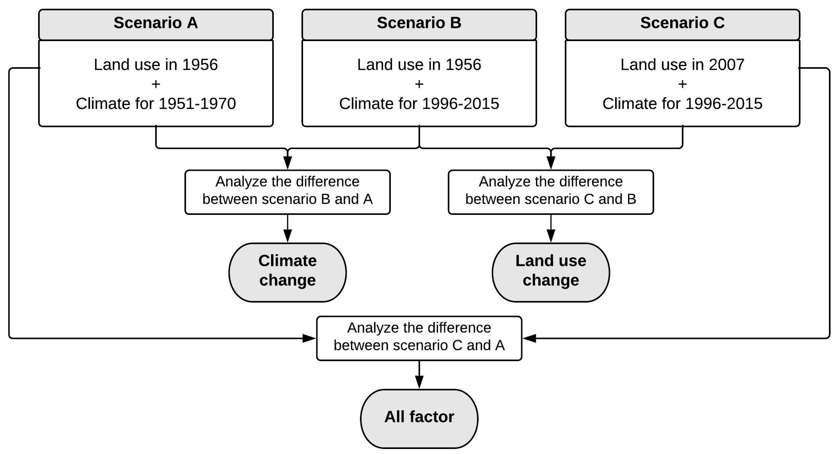
2.4. Framework for Separating Effects of Climate Change and LULC

As can be seen in Figure 2, to study climatic and land uses’ impacts on water resources in the HWSRB, three simulation experiments were set up as follows: scenario A used land use and climate conditions around the 1950s and 1960s (land use in 1956 and weather/climate for 1951–1970); scenario B fixed land use in 1956 and actual weather conditions for 1996–2015; and scenario C used land use in 2007 and actual climate conditions for 1996–2015. Based on these scenarios, we analyzed the impacts on water resources due to climate variability (the differences between B and A), reforestation (the difference between C and B), and all factors (the difference between C and A) respectively. This approach of “one factor at a time” has been successfully applied in many studies to evaluate the effects of land-use change and climate variability on hydrology [11,12,50].

3. Results

3.1. Climate Variability in the HWSRB

Climate trend analysis requires a minimum of 15–30 years for accurate results [51]. In this study, the annual and monthly precipitation, temperature, and streamflow trended for the period 1951–2015 were analyzed using the MK test. The values of the MK test statistic (Test Z) and Sen’s slope for various months are provided in

Table 1. Trend analysis results.

Month	Precipitation			Maximum Temperature			Minimum Temperature			Streamflow
	Test Z	Sig.	${\mathit{Q}}_{\mathit{i}}$	Test Z	Sig.	${\mathit{Q}}_{\mathit{i}}$	Test Z	Sig.	${\mathit{Q}}_{\mathit{i}}$	Test Z	Sig.	${\mathit{Q}}_{\mathit{i}}$
January	−0.42		−0.19	−0.53		−0.01	−1.74	a	−0.02	−0.98		−0.03
February	0.06		0.03	−0.42		−0.01	−1.78	a	−0.02	−1.12		−0.03
March	−1.46		−0.51	1.00		0.02	−2.78	c	−0.02	−1.32		−0.05
April	−0.70		−0.17	1.22		0.02	−1.14		−0.01	−1.14		−0.03
May	0.59		0.17	1.27		0.02	−0.12		0.00	0.30		0.00
June	−2.26	b	−0.33	3.95	d	0.06	1.55		0.01	1.13		0.01
July	−1.48		−0.04	3.43	d	0.04	−0.43		−0.01	1.61		0.01
August	0.03		0.00	3.39	d	0.04	1.03		0.01	1.83	d	0.01
September	0.43		0.07	−0.29		0.00	−0.35		0.00	0.23		0.00
October	−0.41		−0.12	0.43		0.01	−0.39		0.00	−0.79		−0.01
November	−0.50		−0.17	−1.39		−0.02	−1.52		−0.02	−1.15		−0.02
December	−1.54		−0.67	−0.59		−0.01	−1.47		−0.02	−1.93	d	−0.05
Annual	−1.59		−2.22	2.16	b	0.02	−1.35		−0.01	−0.67		−0.12

Test Z is the Mann–Kendall (MK) test statistic; $Q_i$ is the Sen’s slope estimator; ^a indicates a significance level of 0.1; ^b indicates a significance level of 0.05; ^c indicates a significance level of 0.01; ^d indicates a significance level of 0.001.

. In terms of precipitation, it can be seen that the greatest slope was in the months of December, March, and June. According to Paredes et al. [52], the strong decrease of rainfall in March is mostly associated with a positive trend of the North Atlantic oscillation (NAO) index. It is observed that eight of the 12 months revealed a decreasing trend. On a seasonal timescale, the most important decreases take place in the summer and winter. Del Río et al. [53] previously suggested these trends. The annual precipitation decreased across the study area with a slope of 2.22 mm/year. Streamflow and precipitation show a similar decreasing trend in the study area. Influenced by the interaction between reforestation and climate variability factors, a large decrease in streamflow is occurring between October and April.

Annual maximum air temperature indicated a significant upward trend at the 5% significant level. In addition, the highest magnitude of the trend was found in June. This result is in accordance with those that Del Río et al. [54] proposed. With the exception of winter months, the maximum air temperature showed a rising trend during the remaining months. The decreasing magnitude of the minimum air temperature was smaller compared with the increasing magnitude of the maximum air temperature. Compared with their monthly changes, the decreasing magnitudes in the cold months were larger than they were in warm months. The decrease of the minimum air temperature was especially significant in March (0.01 level of significance).

In summary, compared with the baseline period of time (1951–1970), the mean annual rainfall in the recent period (1996–2015) decreased by 81 mm, whereas the mean annual temperature in the HWSRB increased by 0.13 °C, indicating that the climate was getting warmer and drier. Both climate change and intensive human activities have contributed to a reduction of the mean annual streamflow in the recent period of about 16%.

3.2. Land-Use Change in the HWSRB

Table 2. The conversion percentage (%) of each land-use type from 1956 to 2007.

Land Cover Type	Area Coverage (km2)		Area Coverage (%)		1956–2007
	1956	2007	1956	2007	Change (km2)	Change (%)
Urban Areas	0.16	0.21	0.07	0.09	0.05	+0.02
Water Bodies	0.00	0.44	0.00	0.19	0.44	+0.19
Agricultural Land	17.04	5.48	7.23	2.32	−11.56	−4.91
Grassland	30.96	36.52	13.13	15.49	+5.56	+2.36
Forests	54.91	89.17	23.29	37.82	+34.26	+14.53
Shrubland	82.16	67.37	34.85	28.57	−14.79	−6.28
Transitional Woodland/Shrub	50.06	34.46	21.23	14.62	−15.6	−6.61
Barren Land	0.49	2.13	0.21	0.90	1.64	0.69

shows the land uses in the HWSRB in 1956 and 2007. Two main trends of LULC existed from 1956 to 2007: the decrease of shrubland and agricultural land and the increase of forests. Compared with 1956, agricultural land, shrubland, and woodland-shrub transitions decreased in areal extent by respective amounts of 11.56, 14.79, and 15.60 km². In contrast, during the period of 1956−2007, the forest area showed an increase of 34.26 km². Urban areas, water bodies, grassland, and barren land changed little compared with their baselines of 1956.

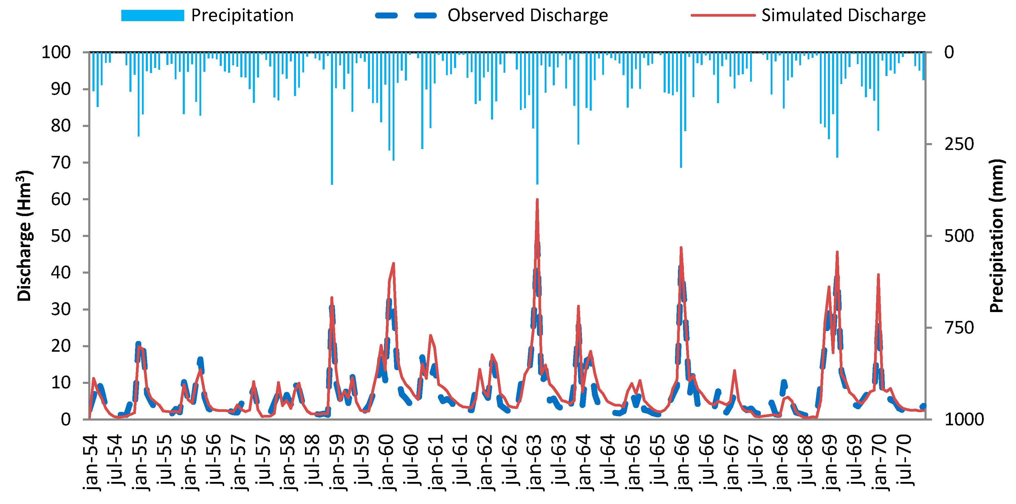
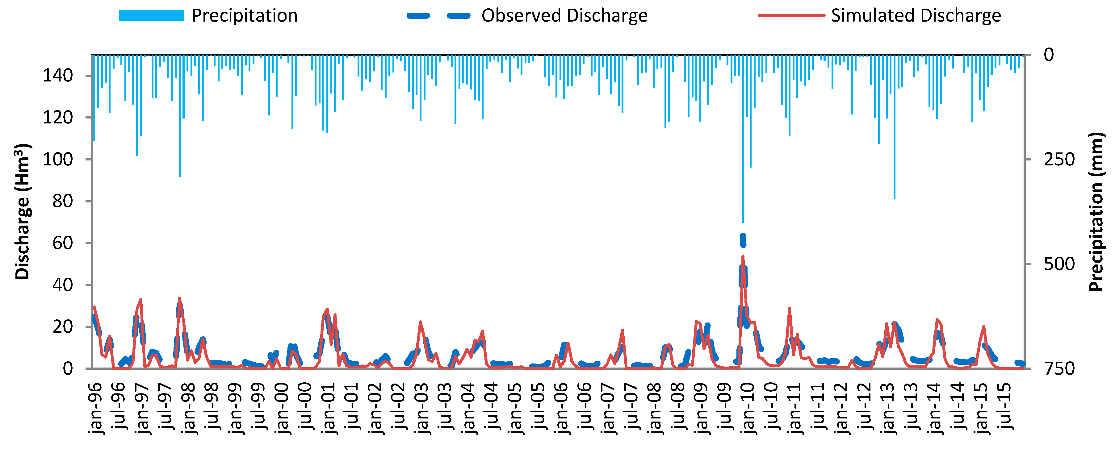
3.3. Validation of the SWAT model

The global sensitivity analysis found that the most influential parameters were the effective hydraulic conductivity in tributary channel alluvium (CH_K1), the U.S. Soil Conservation Service curve number (CN2), the moist bulk density (SOL_BD), the saturated hydraulic conductivity (SOL_K), the groundwater delay (GW_DELAY), the maximum canopy storage (CANMX), the lateral flow travel time (LAT_TTIME), and the available water capacity of the soil layer (SOL_AWC). Similar parameters were chosen for calibration in basins with similar characteristics [55]. Even the sensitivity analysis did not give the soil evaporation compensation factor (ESCO) as one of the most sensitive parameters, but it was considered to be a significant parameter because it is highlighted in the literature and in previous work made for this basin [5,56]. Sensitivity analysis was followed by automatic calibration. The optimal values and range of parameters are presented in

Table 3. Calibration parameters.

Parameter	Description	Value Range	Adjusted Value
CH_K1	Effective hydraulic conductivity in tributary channel alluvium	0–300	17.94
LAT_TTIME	Lateral flow travel time	0–180	109.95
CN2	SCS runoff curve number	–20%–+20%	+8.75%
SOL_K	Saturated hydraulic conductivity	0–2000	0.054
GW_DELAY	Groundwater delay (days)	0–500	242.46
CANMX	Maximum canopy storage	0–100	8.65
SOL_AWC	Available water capacity of the soil layer	0–1	0.0567
SOL_BD	Moist bulk density	0.9–2.5	2.40
ESCO	Soil evaporation compensation factor	0–1	0.5725

.

According to

Table 4. Performance of Soil and Water Assessment Tool (SWAT) model during calibration and validation periods in the HWSRB.

Period	R	NSE	PBIAS	RSR
Calibration (1954–1963)	0.87	0.86	−14.11	0.38
Validation (1964–1970)	0.93	0.88	−17.23	0.35

NSE: Nash-Sutcliffe coefficient; PBIAS: percent bias; RSR: RMSE-observations standard deviation ratio.

, the SWAT model performed well in both the calibration and the validation period, accurately simulating the discharge after the sensitive parameters were optimized. The R, NSE, PBIAS, and RSR of the calibration period (1954–1963) for monthly runoff were 0.87, 0.86, −14.11%, and 0.38 respectively. Overall, the model had good performance not only during the calibration period but also during the validation period. This is not usual because parameters are optimized during calibration, and better performance is expected during this period [57,58]. The results suggest that the SWAT model performed well and can be used for further analysis in the HWSRB.

To illustrate the model calibration and validation, observed and simulated monthly discharge data in the Anchuricas Reservoir for the calibration (1954–1963) and validation (1964–1970) periods are plotted in Figure 3.

As can be seen in Figure 4, we have also validated the model by comparing the simulated results using the 2007 land-use map (scenario C) with observed streamflows during the period 1996–2015. The values of model evaluation statistics such as NSE, R, PBIAS, and RSR were 0.72, 0.85, 21.93, and 0.53, respectively. These values indicate that the calibrated model satisfactorily simulates the monthly runoff.

3.4. Impacts of Land-Use Change and Climate Variability on Runoff and ET at HWSRB

Table 5. Simulated average annual runoff and ET under various scenarios (mm).

Scenarios	Climate	LUCC	P	Runoff	ET	Runoff Change	ET Change
A	1951–1970	1956	895.4	363.7	493.1
B	1996–2015	1956	814.1	302.0	479.9	–61.7	−13.2
C	1996–2015	2007	814.1	267.9	524.9	–95.8	+31.8

LUCC: land-use land-cover changes; ET: evapotranspiration.

shows the annual mean runoff and ET simulated by SWAT under the three different scenarios analyzed in this study. Following the recommendation of Li et al. [59], the simulated data rather than observed data were used to compare the hydrological effects under the three hypothetical scenarios presented in Section 2.4. Compared with the baseline scenario (Scenario A), simulated runoff in Scenario C decreased by 95.8 mm. This reduction is due to the combined effects of climate variability and the reforestation plan. The contrast between Scenarios A and B showed the influence of the climate variability. Surface runoff decreased significantly by 61.7 mm due to climate variation, which accounted for 64.4% of the total runoff reduction. The results revealed that the reforestation plan and climate variability both decreased the runoff. It should be noted that the contribution of climate variability (61.7 mm) is almost two times greater than that of the reforestation plan (34.1 mm). In terms of ET, the combined effect of land-use change and climate variation increased ET by 31.8 mm. The climate variation caused a decrease of 13.2 mm in the ET mainly due to the significant decrease in the precipitation shown in the trend analysis, and in spite of the slight temperature increase. It should also be noted that the reforestation plan contributed to an increase in the ET values by about 45 mm, exceeding by far the impact of climate variability on ET. These results are consistent with those of previous studies [22,23].

4. Conclusions

Considering the HWSRB, as a case study, the aim of this study was to distinguish the influences of human activities and climate variability on water resources by using the SWAT model. From the results of this study, the following conclusions can be stated:

• The SWAT model was able to reproduce the hydrological conditions of the HWSRB. The statistical results of calibration were NSE = 0.86, RSR = 0.38, and PBIAS = −14.11. The validation results were NSE = 088, RSR = 0.35, and PBIAS = −17.23. These results are indicative of the SWAT model’s good performance.
• The main trend in land cover change was the conversion of agricultural areas and shrubland to forest, both of which are a result of the reforestation plan carried out during the 1970s.
• In general, climate change and reforestation activities tend to decrease the streamflow of the HWSRB. The contributions of climate change (64.4%) were larger than that of the reforestation plan (35.6%).
• The results also revealed that the reforestation plan had a higher impact than climate variability did on ET in the HWSRB.
• Although reforestation plans can result in decreased soil erosion rates, runoff is also reduced. The results obtained from this study may have strong implications for a basin that is already suffering from high water stress. The impacts of the reforestation plan should be incorporated into water resource management plans to develop sustainable strategies.
• Future reforestation plans in this area should strengthen the native shrub type of vegetation instead of increasing the forested area in order to preserve the water yield.

References

1. Li, Y.Y.; Chang, J.X.; Wang, Y.M.; Jin, W.T.; Guo, A.J. Spatiotemporal impacts of climate, land cover change and direct human activities on runoff variations in the Wei River Basin, China. Water 2016, 8, 220. [Google Scholar] [CrossRef]
2. Li, Z.; Deng, X.; Wu, F.; Hasan, S.S. Scenario analysis for water resources in response to land use change in the middle and upper reaches of the Heihe River Basin. Sustainability 2015, 7, 3086–3108. [Google Scholar] [CrossRef]
3. Yang, L.; Feng, Q.; Yin, Z.; Wen, X.; Si, J.; Li, C.; Deo, R.C. Identifying separate impacts of climate and land use/cover change on hydrological processes in Upper Stream of Heihe River, northwest China. Hydrol. Process. 2017, 31, 1100–1112. [Google Scholar] [CrossRef]
4. Giorgi, F.; Lionello, P. Climate change projections for the Mediterranean region. Glob. Planet. Chang. 2008, 63, 90–104. [Google Scholar] [CrossRef]
5. Senent-Aparicio, J.; Pérez-Sánchez, J.; Carrillo-García, J.; Soto, J. Using SWAT and Fuzzy TOPSIS to assess the impact of climate change in the headwaters of the Segura River Basin (SE Spain). Water 2017, 9, 149. [Google Scholar] [CrossRef]
6. Serra, P.; Pons, X.; Sauri, D. Land-cover and land-use change in a Mediterranean landscape: A spatial analysis of driving forces integrating biophysical and human factors. Appl. Geogr. 2008, 28, 189–209. [Google Scholar] [CrossRef]
7. Morán-Tejeda, E.; Ceballos-Barbancho, A.; Llorente-Pinto, J.; López-Moreno, J.I. Land-cover changes and recent hydrological evolution in the Duero Basin (Spain). Reg. Environ. Chang. 2012, 12, 17–33. [Google Scholar] [CrossRef]
8. García, C.; Amengual, A.; Homar, V.; Zamora, A. Losing water in temporary streams on a Mediterranean island: Effects of climate and land-cover changes. Glob. Planet. Chang. 2017, 148, 139–152. [Google Scholar] [CrossRef]
9. Senent-Aparicio, J.; Pérez-Sánchez, J.; Bielsa-Artero, A.M. Assessment of Sustainability in Semiarid Mediterranean Basins: Case Study of the Segura Basin, Spain. Water Technol. Sci. 2016, 7, 67–84. [Google Scholar]
10. Woldesenbet, T.A.; Elagib, N.A.; Ribbe, L.; Heinrich, J. Hydrological responses to land use/cover changes in the source region of the Upper Blue Nile Basin, Ethiopia. Sci. Total Environ. 2017, 575, 724–741. [Google Scholar] [CrossRef] [PubMed]
11. Zhang, L.; Karthikeyan, R.; Bai, Z.K.; Srinivasan, R. Analysis of streamflow responses to climate variability and land use change in the Loess Plateau region of China. Catena 2017, 154, 1–11. [Google Scholar] [CrossRef]
12. Zhao, A.Z.; Zhu, X.F.; Liu, X.F.; Pan, Y.Z.; Zuo, D.P. Impacts of land use change and climate variability on green and blue water resources in the Weihe River Basin of northwest China. Catena 2016, 137, 318–327. [Google Scholar] [CrossRef]
13. Yin, Z.; Feng, Q.; Yang, L.; Wen, X.; Si, J.; Zou, S. Long Term Quantification of Climate and Land Cover Change Impacts on Streamflow in an Alpine River Catchment, Northwestern China. Sustainability 2017, 9, 1278. [Google Scholar] [CrossRef]
14. Molina-Navarro, E.; Trolle, D.; Martínez-Pérez, S.; Sastre-Merlín, A.; Jeppesen, E. Hydrological and water quality impact assessment of a Mediterranean limno-reservoir under climate change and land use management scenarios. J. Hydrol. 2014, 509, 354–366. [Google Scholar] [CrossRef]
15. Salmoral, G.; Willaarts, B.A.; Garrido, A.; Guse, B. Fostering integrated land and water management approaches: Evaluating the water footprint of a Mediterranean basin under different agricultural land use scenarios. Land Use Policy 2017, 61, 24–39. [Google Scholar] [CrossRef]
16. Boix-Fayos, C.; de Vente, J.; Martinez-Mena, M.; Barbera, G.G.; Castillo, V. The impact of land use change and check-dams on catchment sediment yield. Hydrol. Process. 2008, 22, 4922–4935. [Google Scholar] [CrossRef]
17. Araque Jiménez, E. Forest landscapes in the Prebetic Arc. The Segura and Cazorla Mountains. Rev. Estud. Reg. 2013, 96, 321–344. (In Spanish) [Google Scholar]
18. Quiñonero-Rubio, J.M.; Nadeu, E.; Boix-Fayos, C.; de Vente, J. Evaluation of the effectiveness of forest restoration and check-dams to reduce catchment sediment yield. Land Degrad. Dev. 2016, 27, 1018–1031. [Google Scholar] [CrossRef]
19. Bosch, J.M.; Hewlett, J.D. A review of catchment experiments to determine the effects of vegetation changes on water yield and evapotranspiration. J. Hydrol. 1982, 55, 3–23. [Google Scholar] [CrossRef]
20. Sahin, V.; Hall, M.J. The Effects of Afforestation and Deforestation on Water Yields. J. Hydrol. 1996, 178, 293–309. [Google Scholar] [CrossRef]
21. Brown, A.E.; Zhang, L.; McMahon, T.A.; Western, A.W.; Verstessy, R.A. A review of paired catchment studies for determining changes in water yield resulting from alteration in vegetation. J. Hydrol. 2005, 310, 28–61. [Google Scholar] [CrossRef]
22. Sun, G.; Zhou, G.; Zhang, Z.; Wei, X.; McNulty, S.G.; Vose, J.M. Potential water yield reduction due to forestation across China. J. Hydrol. 2006, 328, 548–558. [Google Scholar] [CrossRef]
23. Llorens, P.; Latron, J.; Oliveras, I. Modelización del efecto del Cambio Global en la hidrología superficial. Ejemplo de aplicación a una cuenca Mediterránea de montaña. In Proceedings of the 3rd Asamblea Hispano-Portuguesa de Geodesia y Geofísica, Valencia, Spain, 4–7 February 2002; García, F., Berné, J.L., Eds.; Universidad Politécnica de Valencia: Valencia, Spain, 2003; Volume 3, pp. 1679–1681. (In Spanish). [Google Scholar]
24. Belmar, O.; Velasco, J.; Martinez-Capel, F. Hydrological classification of natural flow regimes to support environmental flow assessments in intensively regulated Mediterranean rivers, Segura River Basin (Spain). Environ. Manag. 2011, 47, 992. [Google Scholar] [CrossRef] [PubMed]
25. Moral, F.; Cruz-Sanjulian, J.J.; Olias, M. Geochemical evolution of groundwater in the carbonate aquifers of Sierra de Segura (Betic Cordillera, Southern Spain). J. Hydrol. 2008, 360, 281–296. [Google Scholar] [CrossRef]
26. Salmi, T.; Maatta, A.; Anttila, P.; Airola, T.R.; Amnell, T. Detecting Trends of Annual Values of Atmospheric Pollutants by the Mann–Kendal Test and Sen’s Slope Estimates—The Excel Template Application MAKESENS; User Manual; Air Quality, Finish Meteorological Institute: Helsinki, Finland, 2002; p. 35. [Google Scholar]
27. Tesemma, Z.K.; Mohamed, Y.A.; Steenhuis, T.S. Trends in rainfall and runoff in the Blue Nile Basin: 1964–2003. Hydrol. Process. 2010, 24, 3747–3758. [Google Scholar] [CrossRef] [Green Version]
28. Jaagus, J. Climatic changes in Estonia during the second half of the 20th century in relationship with changes in large-scale atmospheric circulation. Theor. Appl. Climatol. 2006, 83, 77–88. [Google Scholar] [CrossRef]
29. Partal, T.; Kahya, E. Trend analysis in Turkish precipitation data. Hydrol. Process. 2006, 20, 2011–2026. [Google Scholar] [CrossRef]
30. Sen, P.K. Estimates of the regression coefficient based on Kendall’s tau. J. Am. Stat. Assoc. 1968, 63, 1379–1389. [Google Scholar] [CrossRef]
31. Dile, Y.; Daggupati, P.; George, C.; Srinivasan, R.; Arnold, J. Introducing a new open source GIS user interface for the SWAT model. Environ. Model. Softw. 2016, 85, 129–138. [Google Scholar] [CrossRef]
32. Narsimlu, B.; Gosain, A.K.; Chahar, B.R. Assessment of future climate change impacts on water resources of upper Sind River basin, India using SWAT model. Water Resour. Manag. 2013, 27, 3647–3662. [Google Scholar] [CrossRef]
33. Arnold, J.G.; Srinivasan, R.; Muttiah, R.S.; Williams, J.R. Large area hydrologic modeling and assessment Part I: Model development. J. Am. Water Resour. Assoc. 1998, 34, 73–89. [Google Scholar] [CrossRef]
34. Zhang, X.; Srinivasan, R.; Hao, E. Predicting hydrologic response to climate change in the Luohe River basin using the SWAT model. Trans. ASABE 2007, 50, 901–910. [Google Scholar] [CrossRef]
35. Abbaspour, K.C.; Rouholahnejad, E.; Vaghefi, S.; Srinivasan, R.; Yang, H.; Klove, B. A continental-scale hydrology and water quality model for Europe: Calibration and uncertainty of a high-resolution large-scale SWAT model. J. Hydrol. 2015, 524, 733–752. [Google Scholar] [CrossRef]
36. Neitsch, S.; Arnold, J.; Kiniry, J.; Williams, J.; King, K. Soil and Water Assessment Tool, Theoretical Documentation, version 2009; Texas Water Resources Institute: College Station, TX, USA, 2005. [Google Scholar]
37. Ritchie, J.T. Model for predicting evaporation from a row crop with incomplete cover. Water Resour. Res. 1972, 8, 1204–1213. [Google Scholar] [CrossRef]
38. Andalusian Network of Environmental Information (REDIAM). Comparador WMS Ortofotos; Cartografía de Inundaciones en Febrero-Marzo 2010 en las Cuencas de los ríos Guadalquivir y Guadalete; Mapa de usos y Coberturas Vegetales Multitemporal. Available online: http://www.juntadeandalucia.es/medioambiente/site/rediam (accessed on 11 January 2018). (In Spanish).
39. Spanish National Geographic Institute (IGN). Plan Nacional de Ortofotografía Aérea. Available online: http://pnoa.ign.es/ (accessed on 3 January 2018). (In Spanish).
40. Nachtergaele, F.O.; Van Velthuizen, H.; Verelst, L.; Wiberg, D. Harmonized World Soil Database, version 1.2; IIASA: Laxenburg, Austria, 2012. [Google Scholar]
41. Peral García, C.; Navascués Fernández-Victorio, B.; Ramos Calzado, P. Serie de Precipitación Diaria en Rejilla Con Fines Climáticos. Nota Técnica 24 de AEMET; Spanish Meteorological Agency (AEMET): Madrid, Spain, 2017. (In Spanish) [Google Scholar]
42. Herrera, S.; Fernández, J.; Gutiérrez, J.M. Update of the Spain02 gridded observational dataset for EURO-CORDEX evaluation: Assessing the effect of the interpolation methodology. Int. J. Climatol. 2016, 36, 900–908. [Google Scholar] [CrossRef]
43. MAGRAMA (Ministerio de Agricultura y Pesca, Alimentación y Medio Ambiente). Sistema de Información del Anuario de Aforo. Available online: http://sig.magrama.es/aforos (accessed on 1 February 2018). (In Spanish)
44. Abbaspour, K.C. SWAT Calibration and Uncertainty Program—A User Manual; SWAT-CUP-2012; Swiss Federal Institute of Aquatic Science and Technology: Dubendorf, Switzerland, 2012. [Google Scholar]
45. Abbaspour, K.; Vaghefi, S.; Srinivasan, R. A guideline for successful calibration and uncertainty analysis for soil and water assessment: A review of papers from the 2016 International SWAT Conference. Water 2018, 10, 6. [Google Scholar] [CrossRef]
46. Nash, J.E.; Sutcliffe, J.V. River flow forecasting through conceptual models. Part I: A discussion of principles. J. Hydrol. 1970, 10, 282–290. [Google Scholar] [CrossRef]
47. Gupta, H.V.; Sorooshian, S.; Yapo, P.O. Status of automatic calibration for hydrologic models: Comparison with multilevel expert calibration. J. Hydrol. Eng. 1999, 4, 135–143. [Google Scholar] [CrossRef]
48. Legates, D.R.; McCabe Jr, G.J. Evaluating the use of “goodness-of-fit” measures in hydrological and hydroclimatic model validation. Water Resour. Res. 1999, 35, 233–241. [Google Scholar] [CrossRef]
49. Moriasi, D.N.; Arnold, J.G.; Van Liew, M.W.; Bingner, R.L.; Harmel, R.D.; Veith, T.L. Model evaluation guidelines for systematic quantification of accuracy in watershed simulations. Trans. ASABE 2007, 50, 885–900. [Google Scholar] [CrossRef]
50. Zang, C.; Liu, J.; Gerten, D.; Jiang, L. Influence of human activities and climate variability on green and blue water provision in the Heihe River Basin, NW China. J. Water Clim. Chang. 2015, 6, 800–815. [Google Scholar] [CrossRef]
51. Anil, A.P.; Ramesh, H. Analysis of climate trend and effect of land use land cover change on Harangi streamflow, South India: A case study. Sustain. Water Resour. Manag. 2017, 3, 257–267. [Google Scholar] [CrossRef]
52. Paredes, D.; Trigo, R.M.; Garcia-Herrera, R.; Trigo, I.F. Understanding precipitation changes in Iberia in early spring: Weather typing and storm-tracking approaches. J. Hydrometeorol. 2006, 7, 101–113. [Google Scholar] [CrossRef]
53. Río, S.D.; Herrero, L.; Fraile, R.; Penas, A. Spatial distribution of recent rainfall trends in Spain (1961–2006). Int. J. Climatol. 2011, 31, 656–667. [Google Scholar] [CrossRef]
54. Rio, S.D.; Herrero, L.; Pinto-Gomes, C.; Penas, A. Spatial analysis of mean temperature trends in Spain over the period 1961–2006. Glob. Planet. Chang. 2011, 78, 65–75. [Google Scholar] [Green Version]
55. Jimeno-Sáez, P.; Senent-Aparicio, J.; Pérez-Sánchez, J.; Pulido-Velazquez, D. A Comparison of SWAT and ANN models for daily runoff simulation in different climatic zones of peninsular Spain. Water 2018, 10, 192. [Google Scholar] [CrossRef]
56. De Almeida Bressiani, D.; Srinivasan, R.; Jones, C.A.; Mendiondo, E.M. Effects of spatial and temporal weather data resolutions on streamflow modeling of a semi-arid basin, northeast Brazil. Int. J. Agric. Biol. Eng. 2015, 8, 125–139. [Google Scholar]
57. Gassman, P.W.; Reyes, M.R.; Green, C.H.; Arnold, J.G. The soil and water assessment tool: Historical development, applications, and future directions. Trans. ASABE 2007, 50, 1211–1250. [Google Scholar] [CrossRef]
58. Molina-Navarro, E.; Martínez-Pérez, S.; Sastre-Merlín, A.; Bienes-Allas, R. Hydrologic modeling in a small mediterranean basin as a tool to assess the feasibility of a limno-reservoir. J. Environ. Qual. 2014, 43, 121–131. [Google Scholar] [CrossRef] [PubMed]
59. Li, Z.; Liu, W.; Zhang, X.; Zheng, F. Impacts of land use change and climate variability on hydrology in an agricultural catchment on the Loess Plateau of China. J. Hydrol. 2009, 377, 35–42. [Google Scholar] [CrossRef]
Figure 1. Location of the headwaters of the Segura River Basin (HWSRB) and its digital elevation model (DEM).
Sustainability 10 03277 g001
Figure 2. Scenarios setup and research framework.
Sustainability 10 03277 g002
Figure 3. Calibration (1954–1963) and validation (1964–1970) results of SWAT model in Anchuricas Reservoir.
Sustainability 10 03277 g003
Figure 4. Observed and simulated monthly discharge data for the period 1996−2015 (scenario C) in Anchuricas Reservoir.
Sustainability 10 03277 g004