1. Introduction
China, the biggest carbon emitter in the world, after realizing the importance and urgency of reducing carbon emissions [
1,
2], has taken relevant measures to cut emissions down [
3,
4]. The carbon dioxide (CO
2) emissions from electricity accounted for over half of total CO
2 emissions from fuel combustion in China, and about one-seventh of total CO
2 emissions from fuel combustion in the world [
5]. According to some future carbon emission scenarios, the electricity sector can be regarded as the biggest carbon emitter from the sector-level perspective [
6]. Thus, a deeper understanding of the decoupling of carbon emission growth from electric output and the main drivers of the decoupling process in China is a matter of cardinal significance.
In previous decomposition literatures, structure decomposition analysis (SDA) and index decomposition analysis (IDA) were the most popular tools to figure out the effects when decomposing [
7,
8,
9,
10,
11,
12]. The IDA method has been widely used in previous studies, successfully quantifying the impact of different issues so far [
13]. Tracking new developments, Ang discussed the method formulation using an index number framework [
14], made a detailed review of various methods, and compared the advantages and disadvantages of various decomposition tools. He concluded that the Logarithmic Mean Divisia Index (LMDI) method was the preferred method, because of its perfect theoretical framework, adaptability, ease of use, and result interpretation, as well as other desirable properties in the context of decomposition analysis [
15]. This is a complete decomposition method without residuals, which was generalized by Sun to analyze energy consumption in China [
13]. Ang and Liu later modified the original model to handle negative values in the LMDI technique [
16]. Many studies then applied this technique due to this advantage; for example, Cansino et al. analyzed the influencing factors of different sectors by using a multisector analysis approach [
17]. Paul and Bhattacharya [
18], Shahbaz, M. [
19], Wang et al. [
11,
12], and Lise [
20] also conducted comprehensive analyses of the carbon emission drivers in India, Portugal, China, and Turkey based on their regional characteristics, respectively. Xu et al. decomposed the changes of China’s energy-related air pollutant (NOx, PM
2.5, and SO
2) emissions into various factors by structural decomposition analysis (SDA) [
21]. Hu et al. calculated the carbon emissions from each fuel and tested the contributions of each factor to carbon emissions in Chongqing after taking the sector differences into consideration [
22]. Wang et al. uncovered the drivers of decoupling between economic growth and carbon emissions in Chinese industry [
23]. Sumabat et al. carried out a decomposition analysis of CO
2 emissions from electricity generation in the Philippines [
24]. Wang et al. investigated the decoupling states between economic growth and water use in Beijing, Shanghai, and Tianjin, China [
25], and identified the socioeconomic drivers of decoupling economic growth from energy consumption in China and India [
26]. In general, most previous CO
2 emission decomposition analysis focused on the social and economic factors, and primarily decomposed the emission changes into four main aspects: population, energy mix, energy intensity, and economic development. However, few studies have taken the sector characteristics into account when carrying out the carbon emission decomposition analysis, even though considering these properties can help policymakers develop more applicable strategies for the electricity sector. To fill this gap, we conducted our research from the perspective of electricity sector characteristics via the modified LMDI model on the basis of the extended Kaya identify [
27], aiming to test the impacts of factors on carbon emissions, such as electric output, energy consumption, and conversion efficiency (instead of social and economic development), along with their contributions to decoupling.
For the decoupling research, Tapio proposed a decoupling analysis theoretical framework for the European Union (EU) to measure the relationship between CO
2 emissions and transport output or economic growth [
28]. Diakoulaki and Mandaraka assessed the decoupling process of CO
2 emissions from the industrial development of the manufacturing sector in the EU [
29]. Lin and Liu investigated the CO
2 emissions of the heavy industry via decomposing the decoupling index model [
30]. Hu et al. applied the Tapio decoupling model to identify the drivers of carbon emissions from China’s product sector [
22]. Zhang et al. analyzed the decoupling state and determined the main factors that influenced the decoupling relationship by combining a decoupling model with the decomposition method [
31]. However, previous studies were conducted primarily through the decoupling elasticity system or the decoupling index analysis method, and few studies compared the applicability and stability for a given region. We tried to perform a comparative stability test on the decoupling indices of the electricity sector to fill the gap. Also, the majority of the relevant literature concentrated on uncovering the decoupling relationship between carbon emissions and GDP (gross domestic product) or the added economic value of a sector. Nevertheless, few of them have focused on discussing the relationship of carbon emissions and sectoral output from the perspective of sector development rather than economic gains.
Since power generation is one of the major sources of CO
2 emissions from fossil fuel combustion [
32], the electricity sector is attracting more attention, which is also becoming an increasingly important topic for researchers. Shrestha and Timilsina analyzed the roles of generation mix and fuel intensity in the thermal power carbon intensity of 12 Asian countries [
33]. Wang et al. identified the socioeconomic drivers of the electricity footprint of China’s industrial sectors from both the consumption side and supply side [
34]. Malla discussed the contributions to electricity CO
2 emissions from three factors: electricity production, electricity generation structure, and the energy intensity of electricity generation to carbon emissions [
32]. Besides, although existing studies have identified the relationship between electricity consumption and economic growth in China [
35,
36], most of the previous research discussed the social and economic development factors that led to changes in electricity production and consumption. They aimed to investigate the relationship between the pollution of the power sector and the socioeconomic system. Most of them discussed the main drivers of electricity CO
2 emissions without considering the characteristics of the electricity power sector. However, the policy implications aimed at this are more targeted and applicable than those of economic and social development when formulating corresponding carbon emission reduction policies in China. So, this paper chose the typical high carbon emission sector—the electricity sector—to measure the impact of electricity generation on carbon emissions.
The rest of the paper is organized as follows.
Section 1 contains the literature review.
Section 2 demonstrates the methods and data source.
Section 3 reveals the results.
Section 4 provides the conclusions and policy implications.
2. Materials and Methods
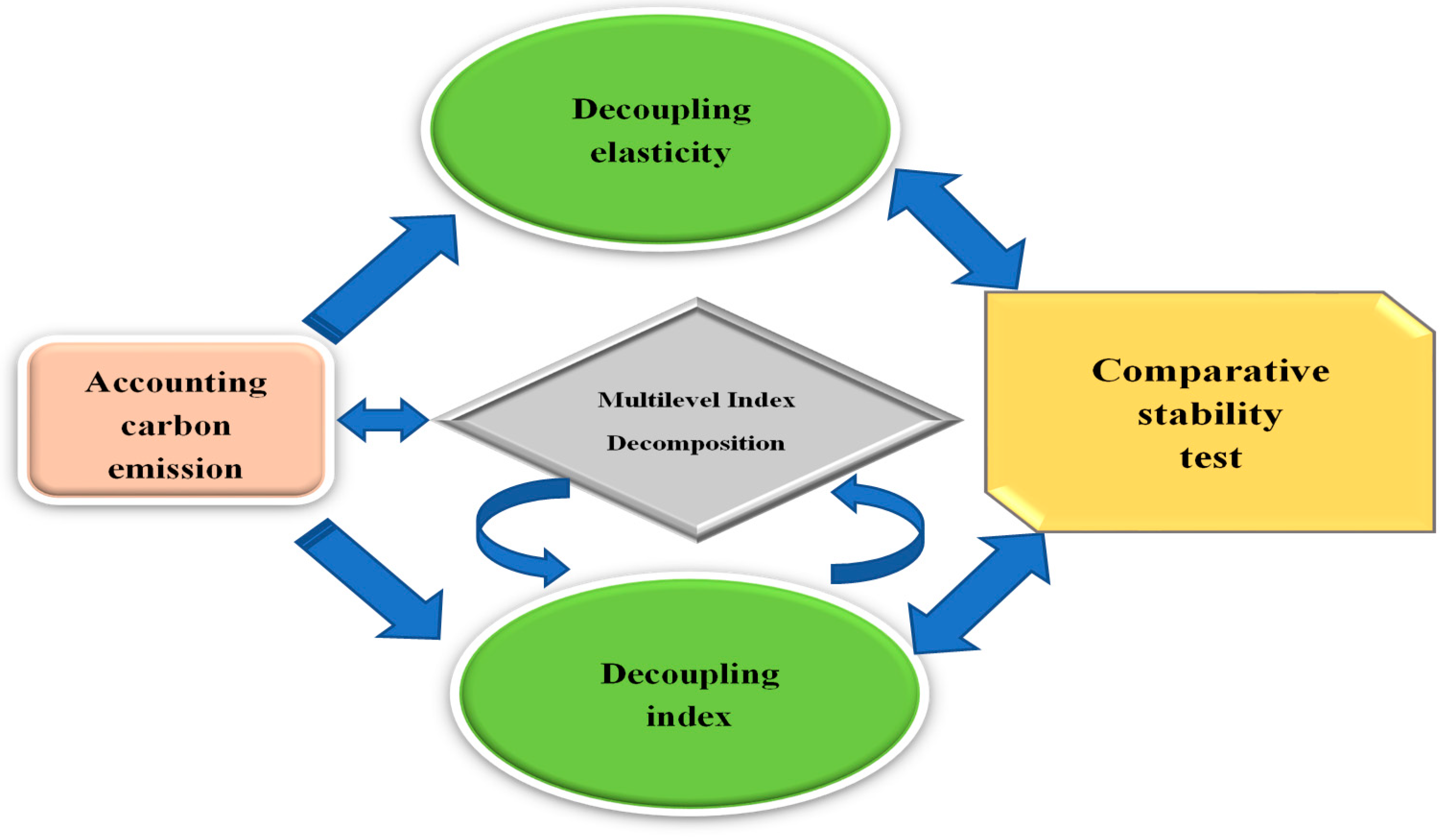
To better display the content and structure of the paper, we drew a proxy diagram to clarify the models applied in this paper (
Figure 1). First, the carbon emissions from fossil fuel combustion in China’s electricity power sector are calculated. Furthermore, the decoupling elasticity model is applied to identify the decoupling states through preliminary calculations of carbon emissions and output from the power sector, and compare the possibilities of reducing or slowing the CO
2 emissions of the electricity sector output. Then, the key drivers of electricity carbon emission changes from the view of the characteristics and development of the electricity sector are investigated by applying the multilevel index decomposition method (additive LMDI and multiplicative LMDI models). The decoupling index model is used to analyze the degree of decoupling (the response and synchronization degree of carbon emissions generated by the power sector to the development and output of the sector), and is then combined with the decomposition model to identify the contributions of various influencing effects. Finally, based on two different decoupling models, the electricity sector in China is used as a pilot issue in order to conduct a comparative stability test of the two widely used decoupling models.
2.1. Energy-Related CO2 Emissions Calculation
The Intergovernmental Panel on Climate Change (IPCC) guidelines [
37] put forward a method for calculating CO
2 emissions from fuels combustion, which is applied to calculate the corresponding CO
2 emissions from electricity production in China in this paper:
and
are the total carbon dioxide emissions from the electric power sector and the carbon emission from fuel
i; and
(million tonnes carbon equivalent, Mtce) is the amount of energy consumed for electricity production from fuel
i. (Kcal/Kg or Kcal/m
3) denotes the carbon emission coefficient of fuel
i;
(tC/TJ) and
represent the carbon content of the calorific value and the oxidation rate of given fuel, respectively, and m is the conversion fraction. The category and emission factor information of each fuel is listed in
Table 1.
2.2. Decoupling Elasticity Index
Using the decoupling elasticity, we established a decoupling model between CO
2 emissions and the output of the electric sector, which is exhibited in Equation (2):
where DE denotes the electric output elasticity of carbon emissions;
and
represent the growth rate of carbon emissions and electric output;
and
are the changes of CO
2 emissions and electricity generation from the base year to the year t; and
,
,
, and
stand for the CO
2 emissions and the output of the electricity sector for the year t and the base year in China, respectively. After considering a 20% variation to avoid regarding a slight change as a significant one, Tapio defined three major decoupling states and eight sub-states. Decoupling can be further divided to three sub-categories: weak decoupling, when carbon emissions and electricity output both increase (0 < decoupling elasticity < 0.8); strong decoupling, when CO
2 emissions grows and electricity output decreases (decoupling elasticity < 0); and recessive decoupling, when carbon emissions and electricity output both decrease (decoupling elasticity > 1.2). Negative decoupling contains three sub-categories: in expansive negative decoupling, CO
2 emissions and electricity output both increase (decoupling elasticity > 1.2); in weak negative decoupling, both variables decrease (0 < elasticity < 0.8); and in strong negative decoupling, CO
2 emissions decrease and electricity volume increases (elasticity < 0). Similarly, coupling is defined as a state that does not over-interpret the slight changes between decoupling and negative decoupling as significant changes, consisting of three sub-states (weak negative decoupling, expansive coupling, and recessive coupling) [
28]. On this basis, the decoupling classification of carbon emissions and electricity output is shown in
Table 2:
2.3. Decoupling Index from Multilevel Index Decomposition
Decoupling index analysis is also an important technique, which was originally advanced by Vehmas [
39] and Diakoulaki [
29]. We aimed to measure the synchronization of the changing trend between environmental deterioration and economic development in China’s electricity sector by calculating the decoupling index.
Firstly, the carbon emission changes from each influencing factor need to be quantified. In general, the CO
2 emission changes from electricity generation can be evaluated by the Logarithmic Mean Divisia Index (LMDI) technique [
11,
40,
41]. Especially, studies have revealed that the LMDI approach showed a relatively satisfying performance when decomposing CO
2 emissions and energy consumption [
15,
42,
43,
44]. In this paper, both additive LMDI and multiplicative LMDI methods from an extended Kaya identity [
45,
46,
47,
48,
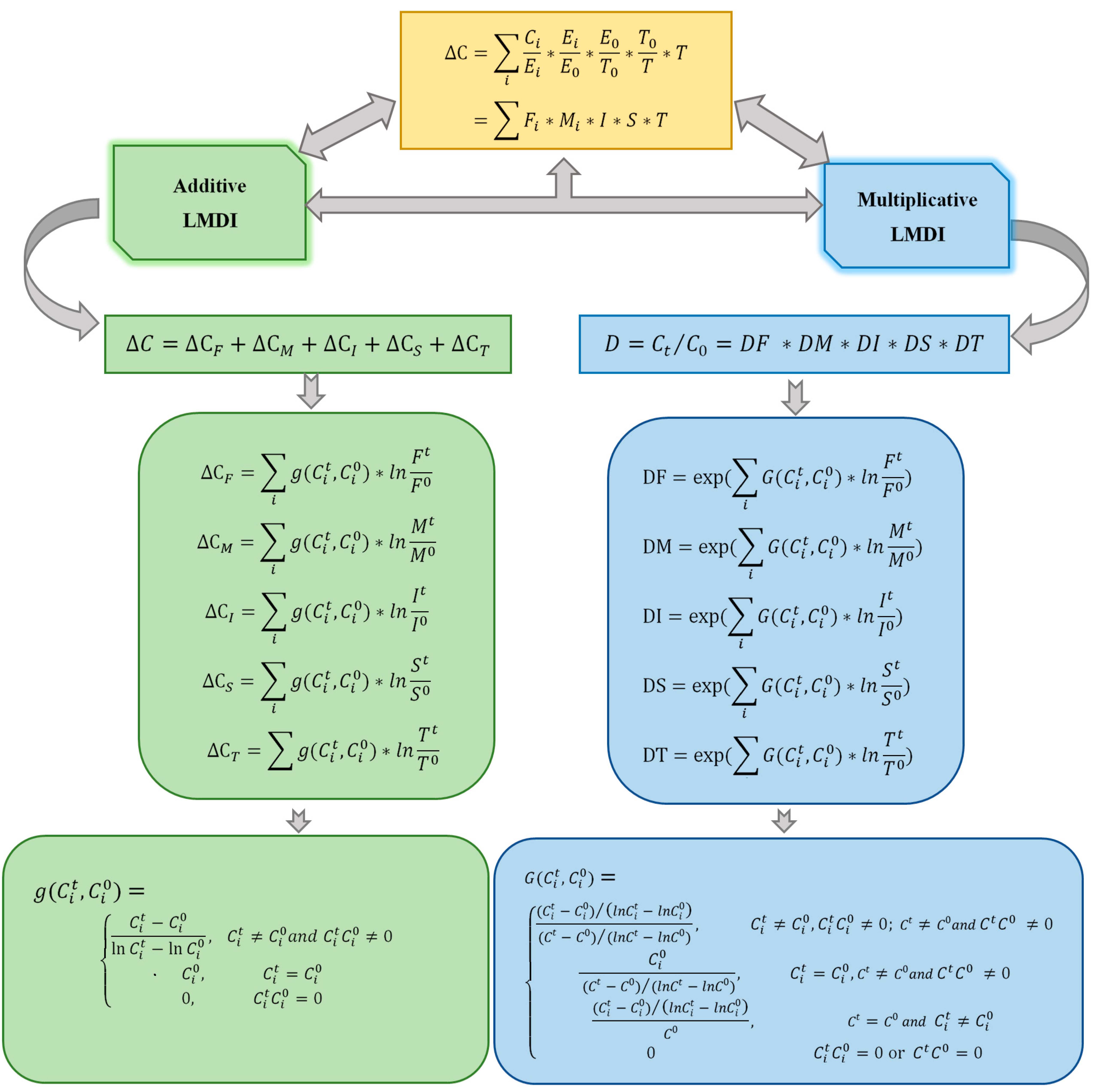
49] were adopted to give a more accurate revelation of the carbon emission changes brought from each effect. Unlike most research on decomposing electricity carbon dioxide emissions, we analyzed the electricity carbon emission from the perspective of the socioeconomic system, discussed the factors such as population and gross domestic product (GDP) per capita, and more importantly, considered the electricity sector characteristics. To be more specific, we modified the original LMDI model to improve the pertinence and applicability when discussing the electricity CO
2 emissions by focusing more on the power sector itself instead of the original factors such as population, GDP per capita, and energy intensity (energy consumption of per GDP added). Furthermore, we conducted the decomposition analysis by discussing factors such as the carbon emission factors, energy mix, gross coal consumption rate, electricity structure, and electricity production. Furthermore, a proxy diagram was drawn to give an easier understanding of the LMDI tools in
Figure 2.
Where represents the total energy consumption amount from thermal power production; and and denote the total electricity production and fire power production, respectively. Consequently, the five effects are: carbon emission factor effect, ); energy mix effect, ; conversion efficiency effect (measured by gross coal consumption rate), I; electricity structure effect, S; and electricity output effect (measured by electricity production), T. , , , , and are the carbon emission changes from the five stated effects; D is the ratio of the electricity CO2 emissions in the year t and the base year; and are the multiplicative decomposition indices from each effect; denotes the estimated weights for the additive LMDI; and represents the estimated weights for multiplicative LMDI.
Due to rapid growth in China between 1995–2012, the CO
2 emissions from electricity generation increased. In this case, the decoupling relationship and its influencing factors need to be identified. The novel decoupling index model combined with the decomposition technique can offer the possibility of measuring the contributions from technology improvement, the energy consumption mix adjustment, or the new electricity generation mode to carbon mitigation. We use
and
to represent the inhibiting effect on CO
2 emissions and the decoupling status of the electric power sector in China during the study period. The calculation method is shown as follows:
where
, and
denote the contributions of the carbon emission factor effect, energy mix effect, conversion efficiency effect, electricity structure effect, and electricity output effect to the decoupling process, respectively.
It should note that if ≥ 1, then a strong decoupling is defined, which means that the mitigation efforts grow faster than the growth of carbon emissions in the electricity generation process. Moreover, when , a relative decoupling state is defined.
In other words, adjustments to measures played a positive role in cutting the carbon emissions down, such as increasing the energy conversion efficiency, improving the technology, replacing traditional high-carbon fuels with new renewable fuels, and optimizing the electricity generation structure. However, the mitigation efforts might not increase as fast as the carbon emission gains from electricity production. In addition, 0 reveals a situation in which the electricity sector produced more and more carbon emissions, but the relevant policies adjustment or technology improvement may not have come along. What’s worse, other effects also contributed to CO2 emission gains when electricity generation increased the emissions. In this situation, the development of China’s electricity sector was mostly considered within the high-carbon combustion mode. The synchronization degree of the electricity generation and relevant environmental results can be measured.
2.4. Comparative Test of the Decoupling Elasticity and Index Stability
2.4.1. Graphic Stability Comparison of Decoupling Elasticity and Decoupling Index
The box plot was applied to compare the degree of stability from two different decoupling models. By analyzing the distribution interval, corresponding curve trajectory, and deviation points, the distribution information of the two decoupling indices in different years can be distinguished.
2.4.2. Decoupling Stability Coefficient
After the graphic scheme, a novel statistical tool was adopted to clarify the stability of each model. The calculation method was expressed in Equation (5):
In Equation (5), denotes the stability coefficient of the decoupling tool j (j = or ); it is a coefficient to uncover the stability degree of a given decoupling tool. N is the population of samples; in this paper, it represents the amount of the studied years, and and are the value of the decoupling indices in the year m and the year after. The smaller the is, the more stable the tested index will be.
2.4.3. T-Test of Decoupling Elasticity and Decoupling Index
A Student’s t-test was employed to further test the stability differences of the decoupling elasticity and the decoupling index. Before performing the Student’s t-test, the prerequisites need to be checked. Firstly, the t-test was applied on the premise of approximately normal distribution. As a result, the normality test is first conducted by checking the normal PP plot, which is a tool to measure the relationship between the expected value and the calculated value. The test is designed to examine whether they were approximately distributed in the same line, in other words, whether a linear relationship exists between them.
The
t-test technique is shown in the following equation:
where
represents the t-statistic,
is the mean of the tested variables,
denotes the specific value mean of the tested decoupling elasticity or decoupling index, and
S and
n mean the variance and the population of the tested value, respectively. We first made the hypothesis H0:
, and the electricity generation elasticity of carbon emissions was zero. The alternative hypothesis was Ha:
. All of the hypothesis and tests were conducted with the confidence level of 95%. The results can be obtained by checking the standard normal distribution table or analyzing the
p value. When
or the
p value is less than 0.05, the null hypothesis is rejected. Meanwhile, the alternative hypothesis can be accepted. If not, the null hypothesis cannot be rejected in this situation. In the decoupling elasticity test, the calculated elasticity also compared the values 0.8 and 1.2. Regarding the decoupling index test, we wanted to test the average performance of the delinking relationship measured by decoupling index, so the null hypothesis H0:
. Also, the alternative
is also given. Regarding China’s electricity decoupling index, a
t-test is also conducted. What’s more, in order to figure out the specific state further, we tested whether the average electricity sector had gotten rid of the linking relationship with the highly reliant development pattern by checking whether the mean value was greater than zero. As a result, we made the null hypothesis that
. Accordingly, the alternative hypothesis was proposed as
. After comparing the corresponding value in the normal distribution table or the
p value, the results could be attained.
2.5. Data Source and Processing
The data used in our study period (1991–2012) were mainly obtained from the General Principles for the Calculation of Comprehensive Energy Consumption [
50] and China Energy Statistical Yearbook [
51]. To be more specific, the total electricity production, thermal power generation, and other energy data such as the consumption amount can be found in the China Energy Statistical Yearbook [
51]. In addition, various fuels are identified to calculate the corresponding carbon emissions. To add more practical meaning to the analysis and develop more feasible measures, after the separate carbon emission calculation, the fuels were merged into three main kinds: coal, oil, and gas. The detailed categories of fuels are listed in
Table 1.
3. Results and Discussion
3.1. The CO2 Emissions from the Electricity Sector
The electricity carbon intensity is defined as the ratio of energy-related carbon emissions from electricity generation to electric output [
52,
53,
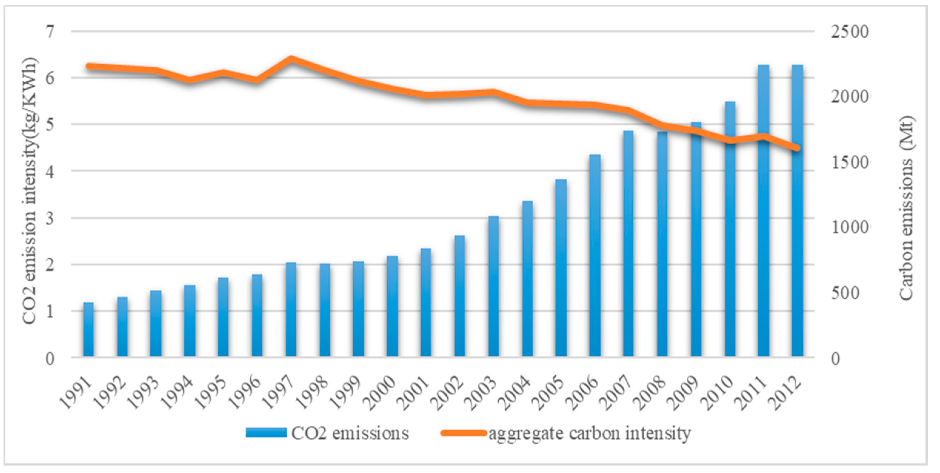
54]. The changing trend in China between 1991–2012 is shown in
Figure 3. As is demonstrated in the figure, the study period can be discussed from three separate spans: 1991–1997, 1998–2007, and 2008–2012. Carbon emissions increased in the first span; meanwhile, carbon emission intensity showed a downward trend.
The carbon dioxide emissions grew faster in the second phase while carbon emission intensity showed a decreasing trend in phase 2, with an average annual growth rate of −1.64%. In this period, CO2 emissions from electricity generation grew with an average annual growth rate of 6.68%; the aggregate carbon intensity also dropped, with an average annual growth rate of 2.59%. However, the overall annual rate of carbon dioxide emissions is 8.25%, and the carbon emission intensity increased at an annual rate of 1.56%.
The slowdown of CO2 emissions represents adjustments such as fuel-switching options and the improvement of the fire-powered technology, but after analyzing the whole period, the amount of the carbon dioxide emissions of the fire-powered electricity plants was still huge.
3.2. Decoupling Elasticity Analysis
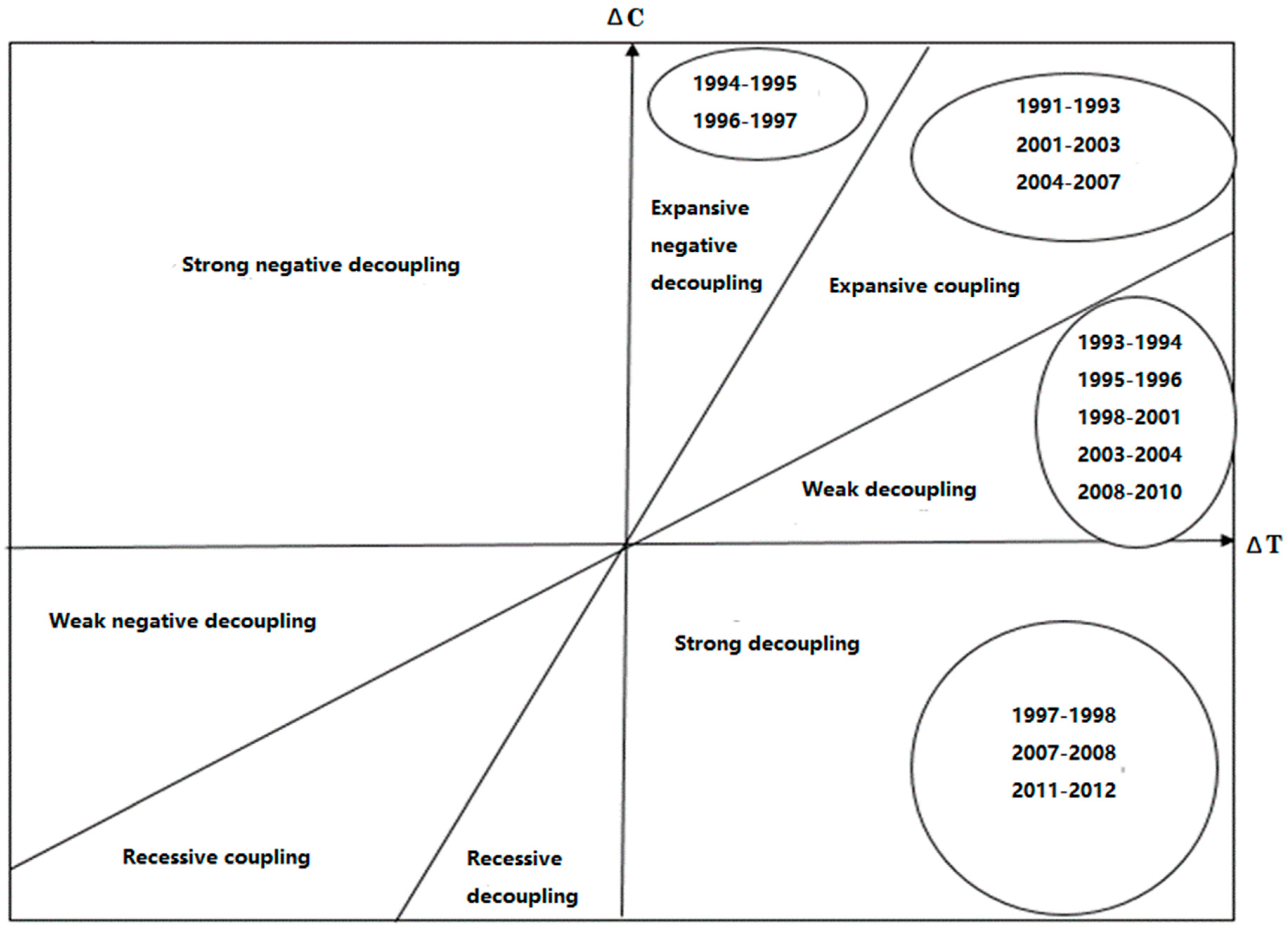
As shown in
Figure 4, the decoupling status varied within the specific timespan; however, the expansive coupling state and the weak decoupling state occurred with higher frequency. In fact, the decoupling state appeared only during 1993–1994, 1995–1996, 1997–2001, 2003–2004, 2007–2010, and 2011–2012. Moreover, the expected strong decoupling state only appeared in 1997–1998, 2007–2008, and 2011–2012. During these years, the link between electric output and corresponding carbon emissions showed a possibility of being broken. Also, since the decoupling elasticity can indicate how the environment responds to the electric output, after the calculation, we found that the decoupling elasticity in most years was around one, indicating that the environment response had a relatively synchronous response to China’s electricity generation in most of the observed years.
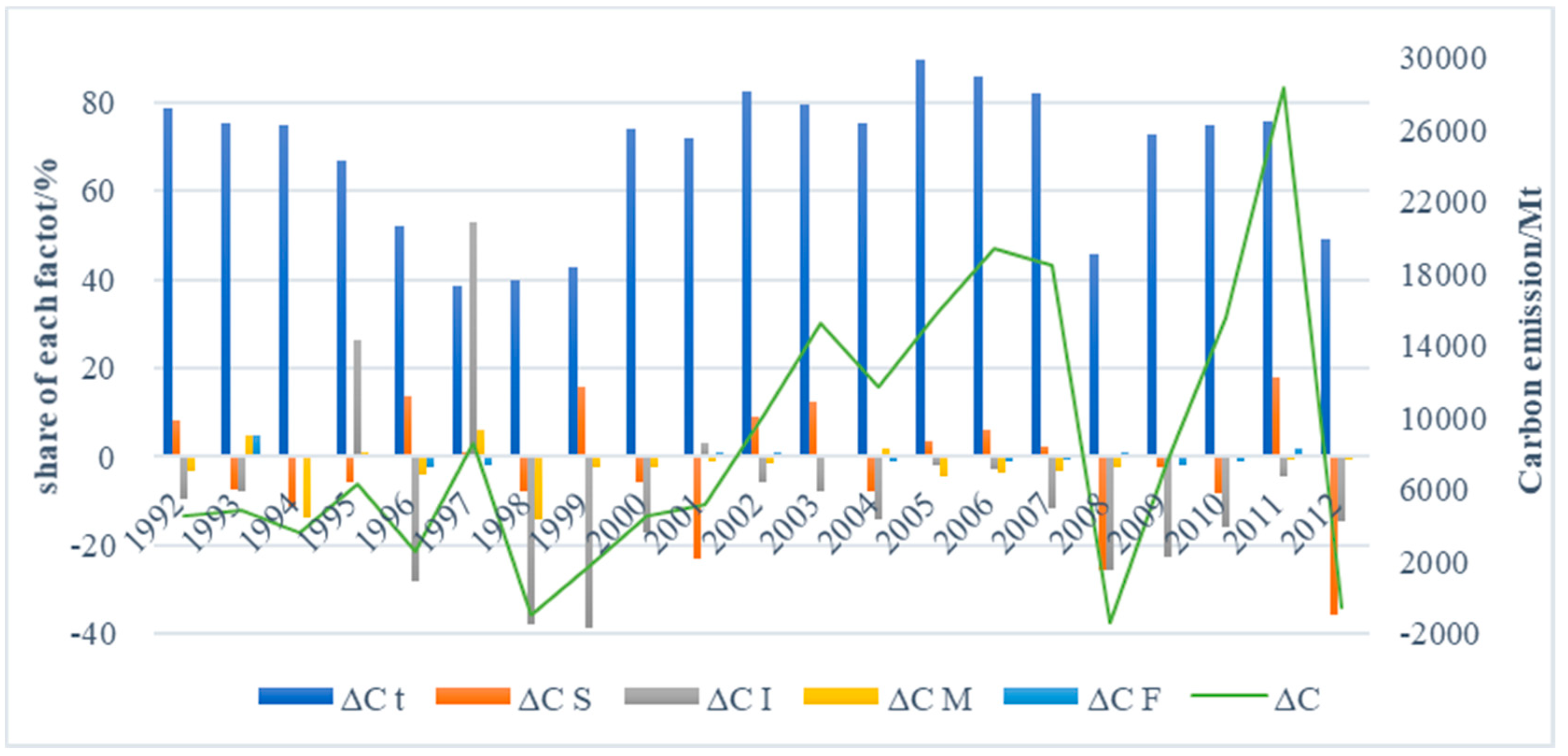
3.3. Drivers of Carbon Emission Identification
The contributions of the five determinants were shown in a bar graph, and corresponding electricity CO
2 emissions were shown as the green line in
Figure 5. The CO
2 emissions increased during 1991–2012 in most years, except for 1998, 2008, and 2012. Besides, between 1991–1997, the changes of the carbon dioxide emissions increased faster than during the other phases at an annual rate of 10.34%. As shown in
Table 3, in general, the electric power output effect contributed most to the increasing electricity carbon dioxide emissions; however, the influence of the other factors varied from year to year. The electricity intensity effect helped to curb the corresponding CO
2 emissions; the CO
2 emission mitigation mainly came from the technology development in electricity generation, which is consistent with the research before [
55,
56]. In addition, energy mix can pose a positive effect on the carbon emission decrease except during the years 1993, 1995, 1997, 2003, and 2004. A switch to fuels with a better generating efficiency also contributed to an efficiency improvement [
55]. Even though the emission factor effect had a relative minor impact, it is closely related to decarbonization of the energy system, and should not be ignored.
3.4. Decoupling Index Analysis
The decoupling index analysis was carried out after measuring the carbon emissions from each effect. The degree of synchronization and the contributions of each effect to the decoupling process can further be uncovered. The decoupling status and the contributions of every influencing factor are shown in
Table 4.
As indicated in the results of the decoupling index analysis, three decoupling states were identified: strong decoupling, no decoupling, and relative decoupling. Strong decoupling offered a possible situation in which the electricity sector developed while the relevant carbon emissions dropped. The strong decoupling state was mainly brought from technological improvement, the upgrading of equipment, or a massive switch to low-carbon content fuels, especially renewables. However, strong decoupling only appeared between 1997–1998, 2007–2008, and 2011–2012. Also, a negative decoupling state occurred between 1994–1995, 1996–1997, 2001–2003 and 2010–2011. The power of factors that hindered the decoupling was stronger than the positive effects of accelerating the decoupling process. Nevertheless, in the rest of the years, the relative decoupling state was detected, indicating that even though some efforts had been made to cut down the carbon emissions, they still did not grow as fast as the electricity product gains. Due to the limitations of equipment and unsettled technology issues, the electricity generation from renewable fuels was not widely used to accelerate the decoupling process.
For the decoupling process, since relative decoupling was the main state during the study period in China’s electricity sector, which reveals the possibility of reducing CO
2 emissions with no downward trend of electricity output and development. Zhang et al. concluded that the electricity generation efficiency effect plays the dominant role in decreasing CO
2 emissions [
55], which is closely connected with technological improvements in electricity generation, indicating that technological innovation and the improvement of facilities usage accelerated the decoupling process of CO
2 emissions and electricity output gains.
Besides,
revealed the share of the electricity intensity effect of the decoupling devotion. In most research years, it exerted a positive impact on carbon emission decoupling from electric output. Also, the electricity generation structure accelerated the decoupling in most of the observed years, which is primarily brought from the carbon emissions that had been cut by electricity generation structure changes in recent years in China [
32]. It should be noted that the electric output in 2012 was 4987.55 GW·h, of which 78.05% was from thermal power. Even though it had already dropped from 81.54% in 1991, the fire-powered electricity generation was still in the dominant position throughout the whole electricity generation process. The energy mix effect (
) had made decoupling efforts in most of the years during the study period, while in the rest of the years, such as 1992, 1994, 1996, 2002, and 2001, it mainly acted as a block to the CO
2 emissions decoupling from electric output. Since energy mix effects have positive effects on CO
2 emissions reduction [
57], especially since the energy-efficiency targets of the 11th Five-Year Plan (approved by the Fifth Plenary, Session of the 16
th Communist Party of China; it is a binding energy conservation target for governments), the switch from massive coal consumption to other fuels such as natural gas also benefited from electricity generation [
58], exerting a great impact on the whole decoupling process.
Although the emission factor effect () did not appear to be as important as the other factors in accelerating decoupling for the moment, it may become more powerful, because decarbonization could be a momentous and radical sustainability goal in the future.
3.5. Comparative Stability Test Results
3.5.1. Decoupling Stability Coefficient Analysis
After the calculation via the method in Equation (10), the results showed the difference in stability between the electricity elasticity of carbon emissions and the decoupling index.
The stability coefficient of the elasticity was 0.91, while the coefficient of the decoupling index was 2.26, revealing that for the stability, the electricity elasticity of CO2 emissions had a better performance. Since , the expected strong decoupling was still not adequate; also, the existing relationship between the development of the electricity sector and relevant carbon emissions needed to be improved in China. The elasticity and decoupling index showed consistent results. For example, after the coupling status occurred between 2001–2003, the relative decoupling state appeared, which was attributed to the efforts made by the government, such as the electricity generation structure adjustment and the energy structure improvement. To sum up, the elasticity tool has a more stable manifestation than the decoupling index, while the decoupling index can measure the decoupling status more systematically.
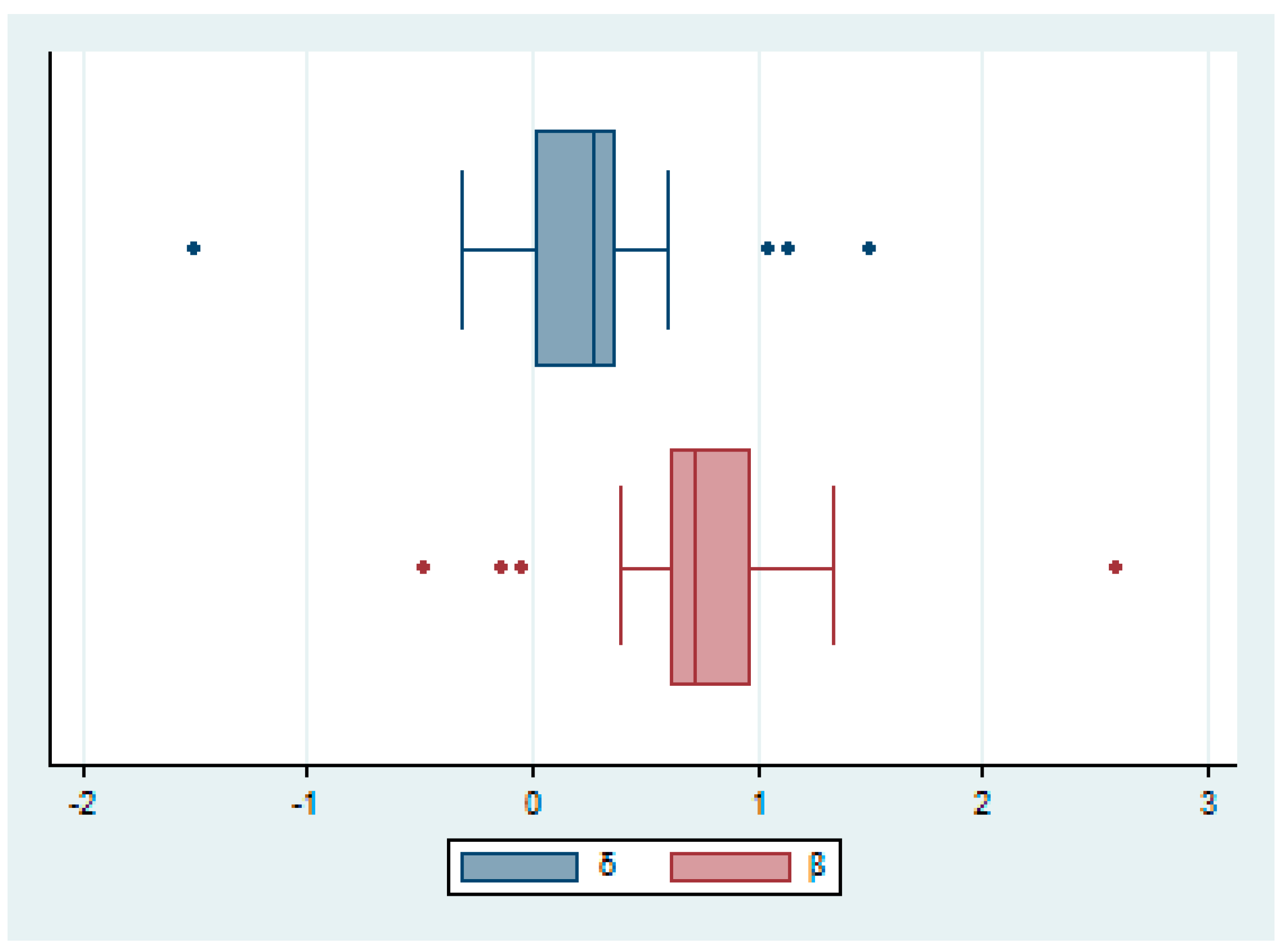
3.5.2. Graphical Results of the Decoupling Indictor’s Stability
As shown in
Figure 6, the outlier data of the decoupling index appeared in 1996–1998, 2007–2008, and 2011–2012. Three of the abnormal points turned out to be in the state of “strong decoupling”, and the abnormal points left showed the status of “no decoupling”, which is consistent with the conclusion that most of the research years showed a relative decoupling state. When it comes to the decoupling elasticity, the abnormal points appeared in same period with the decoupling index; similarly, three points were demonstrated in the state of “strong decoupling”, and one abnormal point presented the “no decoupling” state. In addition, the median of decoupling is between zero and one, implying that the distribution is around the relative decoupling state. What’s more, by analyzing the upper quartile, the lower quartile, and the interquartile range, we figured out that the decoupling index is mostly distributed in an area that is less than one, representing the “relative decoupling” state or the “no decoupling” state. Overall, the decoupling process is not enough, suggesting that effective and promising measures and plans should be put into practice.
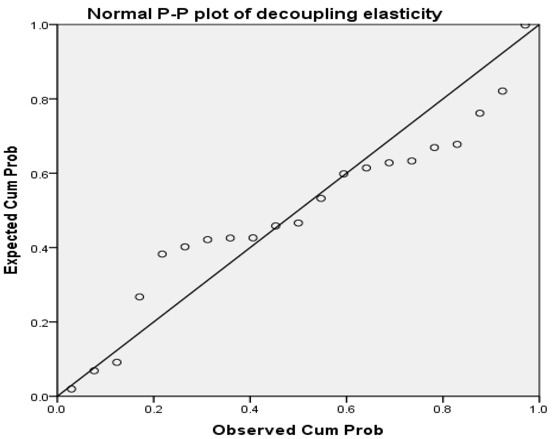
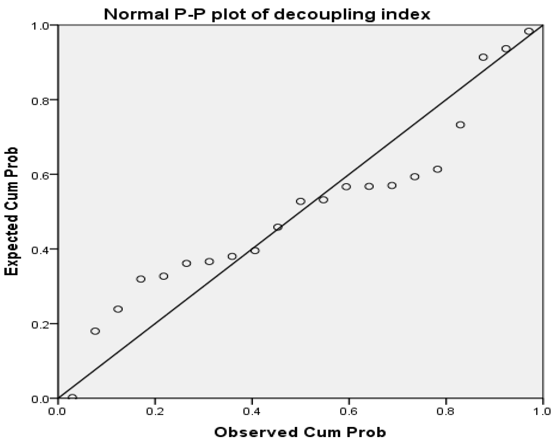
3.5.3. T-Test Analysis of the Decoupling Indices
By analyzing the results of the PP plot in
Figure 7 and
Figure 8, the two indicators can approximately be considered as the normal distribution.
After comparing the
p value with the significance level (0.05), we found that for the elasticity value, the null hypothesis was rejected, and the alternative hypothesis was adopted instead (shown in
Table 5). This means that in most of the studied years, it could not get to the strong decoupling state.
Moreover,
Table 6 and
Table 7 show the test results for testing the decoupling index with one and zero, in which the
p values (0.0000 and 0.0448, respectively) were all smaller than the significance level (0.05). The alternative hypotheses were accepted at this significance level. This indicates that relative decoupling occurred more frequently, which was due to some technological improvement and the effect of the energy policies; there is still a long way to go to achieve the “perfect decoupling state”. In a nutshell, more relevant policies should be developed in the future in consideration of the present situation to realize the goal of increasing the electricity production while also cutting the carbon emissions down.
However, several questions remain that we cannot currently thoroughly investigate. To be more specific, not all of the influencing factors can be analyzed due to the limitation of Kaya identity (must be divided into several multiplications). In this case, we can only select the key factors to carry out our study after a detailed review of the previous research that is related to similar topics. In future research, we will try to further our research by taking more spatial issues such as the spatial stratified heterogeneity phenomenon and spatial autocorrelation into consideration. Also, we will try to focus more on the provincial differences, the carbon emission mitigation performance, and responsibility allocation in future work.


