Article

The Significance of a Building’s Energy Consumption Profiles for the Optimum Sizing of a Combined Heat and Power (CHP) System—A Case Study for a Student Residence Hall

1
Department of Mechanical Engineering, Mirpur University of Science and Technology (MUST), Mirpur 10250 (AJK), Pakistan
2
Faculty of Engineering, Science and the Built Environment, London South Bank University, 103 Borough Road, London SE1 OAA, UK
3
Department of Electrical Engineering, Mirpur University of Science and Technology (MUST), Mirpur 10250 (AJK), Pakistan
4
School of Electrical Engineering and Computer Science, National University of Sciences and Technology (NUST), Islamabad 44000, Pakistan
*
Author to whom correspondence should be addressed.
Sustainability 2018, 10(6), 2069; https://doi.org/10.3390/su10062069
Submission received: 28 May 2018 / Revised: 11 June 2018 / Accepted: 16 June 2018 / Published: 19 June 2018

Abstract

:
University buildings, such as student residence halls with year-round consistent energy demands, offer strong opportunities for Combined Heat and Power (CHP) systems. The economic and environmental feasibility of a CHP project is strongly linked with its optimum sizing. This study aims to undertake such an assessment for a CHP system for a student residence hall located in London, the United Kingdom (UK). The study also aims to undertake a sensitivity analysis to investigate the effect of different parameters on the project’s economics. Necessary data are collected via interviews with the University’s Energy Manager. Modeling of the CHP system is performed using the London South Bank University (LSBU, London, the UK) CHP model. Results demonstrate that optimum sizing of CHP is crucial for achieving higher economic and environmental benefits and strongly depends on the authenticity of the energy consumption data, based on which the CHP is being sized. Use of incorrect energy data could result in an undersized or oversized CHP system, where an oversized system will result in higher negative results compared to an undersized system. Finally, Monto Carlo statistical analysis shows that electricity price is the significant factor that could affect the project’s economics. With an increasing spark gap, the payback period decreases, and vice versa.

1. Introduction

The higher education (HE) sector of the United Kingdom (UK) is comprised of 161 universities. Buildings in the HE sector consume electricity and gas and are responsible for scope 1 (electricity related emissions) and scope 2 emissions (fuel related emissions). In 2010, the HE funding councils (HEFCs, the UK) introduced a 43% carbon reduction target for the year 2020 compared to 2005/06 and linked the capital funding of universities to this target [1]. Since then, the universities in the UK have been implementing a range of carbon reduction projects, which mainly include energy efficiency measures and installation of renewable and clean technologies, such as solar, wind, biomass and Combined Heat and Power (CHP). Figure 1 presents energy consumption of the residential and non-residential buildings of the HE sector in different academic years in terms of kWh/m2.
It is apparent that the sector’s carbon emissions and energy consumption in both types of buildings have been declining, as a result of different carbon reduction initiatives taken by the universities. The trends shown in Figure 1 also unlock another interesting fact that the decrease in annual energy consumption in the residential buildings is almost double that in the non-residential buildings. This is probably because the residential buildings are occupied for the whole year, and therefore, these have been given more priority than the non-residential buildings in terms of energy efficiency measures and installation of renewable and clean technologies, such as CHP. Universities that have installed CHP plants are making good moves towards their carbon reduction targets.
Figure 2 shows the CHP generation and the number of universities that have had installed CHP in different years.
It is apparent that due to the increased number of installation, energy generation from CHP plants has been increasing. In 2008, only 28 universities had CHP and the total energy generation from onsite CHP plants was 685 GWh. This CHP installation number increased to 67 in 2015 with total energy generation of 912 GWh (33% increase). This clearly demonstrates that CHP is being recognized in the HE sector as a leading source for reducing the sector’s carbon emissions. However, on the other hand, installation of CHP in only 67 universities out of 161 universities indicates that this clean energy technology is yet facing some challenges and barriers in the HE sector of the UK. Such barriers were identified by Amber and Parkin [3]. Surprisingly, one of the major barriers identified was lack of support from universities’ higher management.
CHP systems generate heat and electricity simultaneously by burning a single fuel source and are nearly 30–40% efficient compared to the conventional systems [4,5,6]. Due to their onsite installation and use of their waste heat, the losses from CHP systems are 16–25% lower than those from the conventional systems, which use two different sources to meet the buildings electrical and thermal demands.
For a CHP system to be feasible for a building or set of buildings, one of the major requirements is that the buildings should have year-round electrical and thermal demands [7]. In this sense, the student residence halls, which occupy nearly 24% space and have a share of 18% in the total energy consumption of a typical university campus [8], offer a good opportunity for the CHP technology due to their consistent and year-round energy demands.
An optimum sized CHP system operating under an optimum control strategy guarantees higher financial and environmental savings. Optimum sizing of CHP must be calculated based on real hourly thermal and electrical demand profiles of the building(s) [9,10]. Where real demand profiles are not available, it becomes highly important to generate estimated but reliable hourly profiles. Such situations include:
  • no data are available at all for both electricity and gas consumption;
  • only yearly electricity and gas consumption data are available;
  • monthly electricity and gas consumption data are available.
Use of incorrect hourly electrical or thermal demand profiles could result in an undersized or oversized CHP system that will struggle to achieve its financial and environmental targets [11]. Many CHP installations are oversized because the facilitated energy demand profile has not been assessed properly. To get the full benefits of CHP, the unit needs to operate to its full potential, and all the power and heat produced have to be fully utilized [12]. There are examples where CHP were improperly sized and failed to achieve their targets. One of such examples is the installation of CHP in a building block in Lambeth Council in London, where CHP was not sized as per the building’s energy demands but was sized equal to the capacity of already installed boilers. Later on, it was found that CHP was oversized [13]. An oversized CHP system may be beneficial if an electricity export option is available. This means that all the extra electricity could be exported to grid. However, this heavily depends on the export tariff. A lower export tariff makes this option unfeasible [14]. On the other hand, an undersized CHP system does not result in higher financial and environmental savings [15].
Owing to the significance of this subject, this study attempts to highlight the significance of the optimum sizing of a CHP system by undertaking a detailed economic and environmental feasibility of the CHP system for a typical student residence hall building located in London, the UK, and aims to show how the use of estimated demand profiles could affect the CHP sizing and the project’s financial and environmental outcomes. The study further aims to undertake a sensitivity analysis in order to identify different parameters that would have significant effects on the project’s economics. It is anticipated that results of this study would be useful for building services engineers and policy makers.

2. Methodology

2.1. Site Selection

The site selected for this study is a student residence hall called “McLaren House” located at the Southwark campus of London South Bank University (LSBU, London, UK) in central London, UK. McLaren House has over 600 non-smoking rooms and is occupied throughout the year. Each room has a window that could be opened fully for the ventilation purpose. It is a naturally ventilated building with no cooling plant installed. Opened in the 1996, the building has a total Gross Internal Area (GIA) of 14,740 m2. Electricity to the building is supplied through a switch room in the basement. The boiler plant room is located on the 10th floor and comprises 3 × 225 kW gas fired space heating ‘Viessmann’ boilers and two gas fired hot water heaters. The site is controlled by a Satchwell (now Schneider Electric) Sigma Building Management System (BMS). Figure 3 shows a front view of McLaren House.
Through multiple site visits and interviews with the University’s Energy Manager, the building’s electricity and gas consumption data and building related information were collected.

2.2. Electricity and Gas Consumption

Figure 4 shows the monthly electricity and gas consumption of McLaren House.
It is apparent that both electricity and gas consumption are higher during the winter months due to high space heating and hot water demand, while electricity and gas consumption are lower in summer as there is only hot water demand.

2.3. Weather Normalization of Energy Usage

Sizing a CHP system based on energy consumption collected from the utility bills and energy meters, without “normalizing” for typical weather conditions, may result in an undersized or oversized CHP plant. A well-known weather normalization method is the Degree Days Method.
Degree days are usually used as a measure of heating or cooling [16]. Degree days have been vastly used by researchers for the purpose of normalization of energy consumption in different sectors [17,18,19,20,21]. Data of Heating Degree Days (HDD)s for the London region were available from [22].
The weather normalization process has been carried out in the following three steps [23].
  • Step-1: establishment of a relationship between five years average HDDs and actual monthly electricity consumption through linear regression.
  • Step-2: determination of a slope and intercept of a linear regression line.
  • Step-3: use of actual HDDs instead of five years average HDDs in the equation of linear regression along with its slope and intercept values, to calculate the monthly normalized electricity consumption. The aforementioned process of weather normalization was used in order to normalize the monthly electricity and gas consumption of McLaren House.

2.3.1. Normalization of Monthly Gas Consumption

Figure 5 shows the relationship between the last five years average HDDs and the monthly gas consumption of the year 2011. A linear relationship is apparent, which clearly suggests that the larger the number of heating degree days, the higher the heating demand and gas consumption will be, and vice versa. The plot provides an equation with a slope and intercept, where “x” denotes the number of monthly HDDs. Using the HDD values for the year 2011, the gas consumption has been normalized. Figure 6 shows the comparison between the actual and normalized monthly gas consumption of McLaren House. The comparison suggests that in 2011, the gas consumption in January, February and November should have been less but was observed higher.
This could be attributed to the fact that these three months were colder than those in previous years. The profiles suggest that during summer months, the actual and normalized gas consumption were almost equal.

2.3.2. Normalization of Monthly Electricity Consumption

Figure 7 shows the relationship between the last five years average HDDs and the monthly electricity consumption for the year 2011.
It is apparent that the relationship between the monthly average HDDs and the monthly electricity consumption is logarithmic. Using the HDD values for the year 2011, the electricity consumption has been normalized. Figure 8 shows the comparison between the actual and normalized monthly electricity consumption of McLaren House. The comparison suggests that in 2011, the electricity consumption in March and May should have been less but was observed higher. This could be due to the fact that these two months were colder compared to those in previous years.

2.4. Development of Hourly Thermal and Electrical Demand Profiles

This is the most important step before CHP sizing could be performed and is the key to the success of a CHP system for getting the sizing right. Correct hourly demand profiles based on real energy consumption data are desired for sizing a CHP system. Hourly profiles on weekdays and weekends were developed by using the half hourly data.

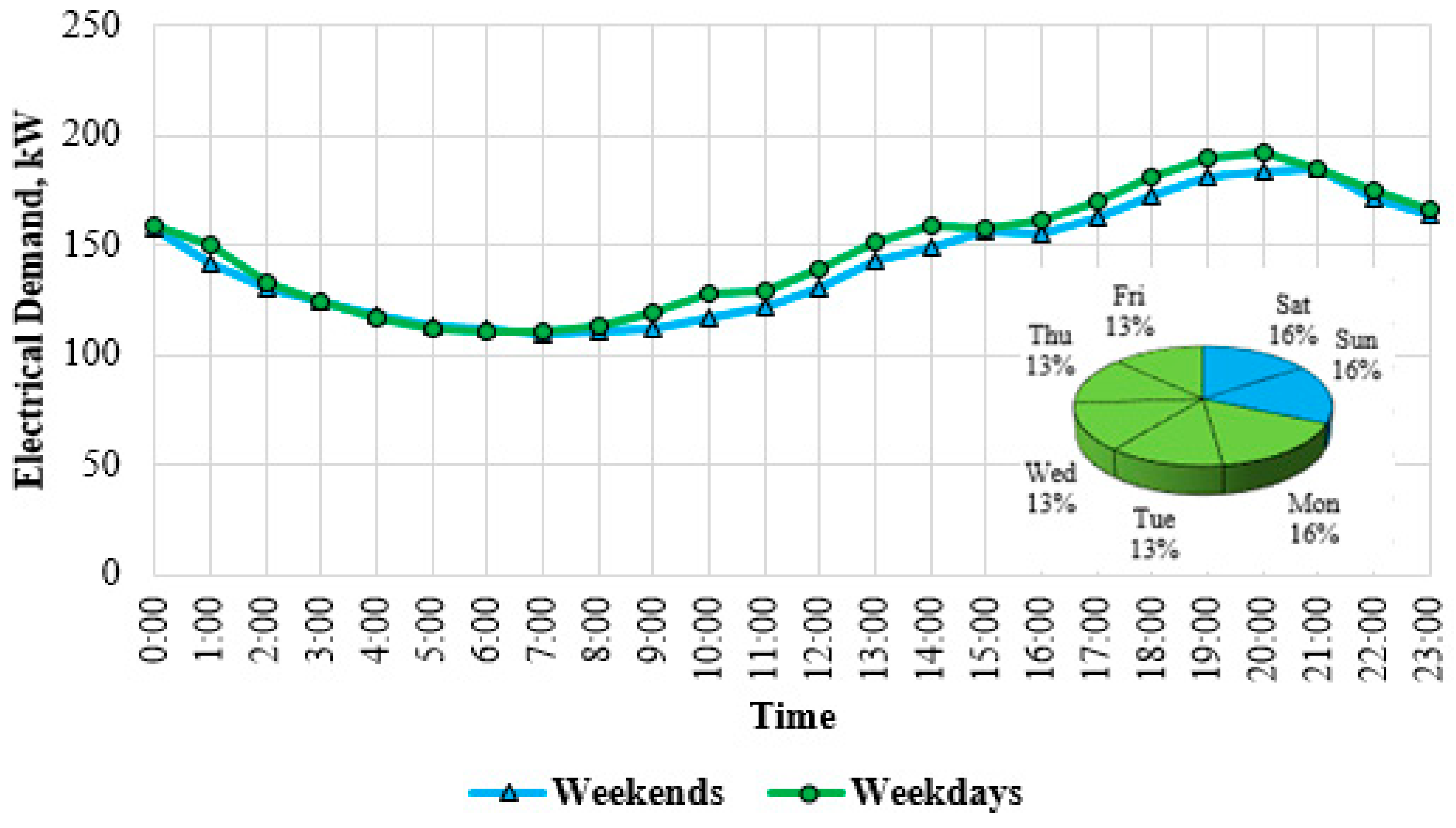
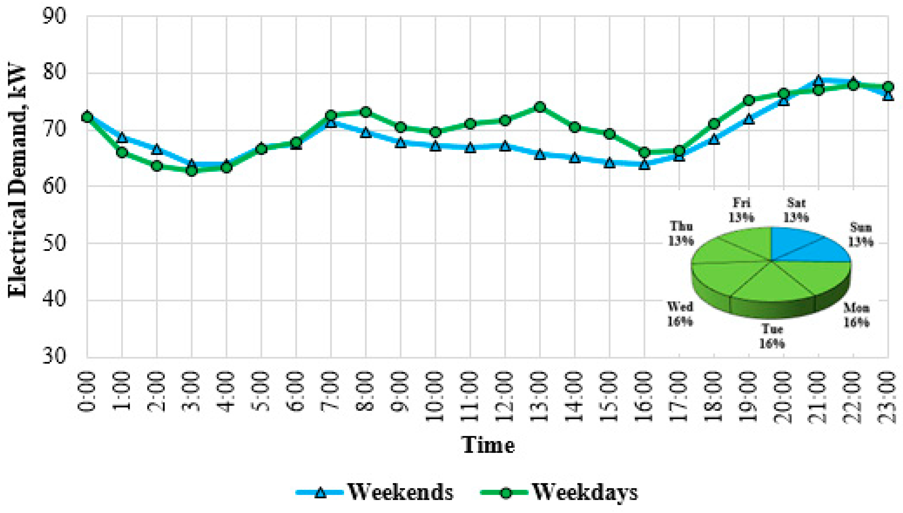
2.4.1. Electrical Demand Profiles

Weekday and weekend hourly electricity demand profiles of McLaren house for the months of January and August are presented in Figure 9 and Figure 10. The following observations can be made.
  • Hourly electricity consumption remains fairly the same on weekdays and weekends with slightly higher consumption on the weekdays.
  • Electricity consumption on a typical weekend is nearly 3% higher than that on a weekday.
  • During winter months, base load remains 100 kW, whereas peak load occurs during evening when the kitchen equipment is under use. The value for the peak load could be as high as 190 kW.
  • During summer months, the base load remains 62 kW, whereas the peak load occurs during evening when the kitchen equipment is under use. The value for the peak load could be as high as 80 kW.
  • During the whole year, the hourly electricity demand remains within 62 kW and 190 kW.

2.4.2. Thermal Demand Profiles

Weekday and weekend hourly thermal demand profiles of McLaren house for a winter and a summer month are presented in Figure 11 and Figure 12. The following observations can be made.
  • Hourly thermal demand remains fairly the same on weekdays and weekends with a slightly higher demand on the weekdays during day period.
  • Thermal demand on a typical weekend is nearly 3% higher than that on a weekday.
  • During winter months, boilers start at 5 a.m. during the whole week. Thermal load remains as high as 630 kW due to high space heating and hot water demand.
  • During summer months, the base load remains between 130–150 kW as there is only hot water demand.
  • During the whole year, hourly thermal demand remains within 130 kW and 700 kW.

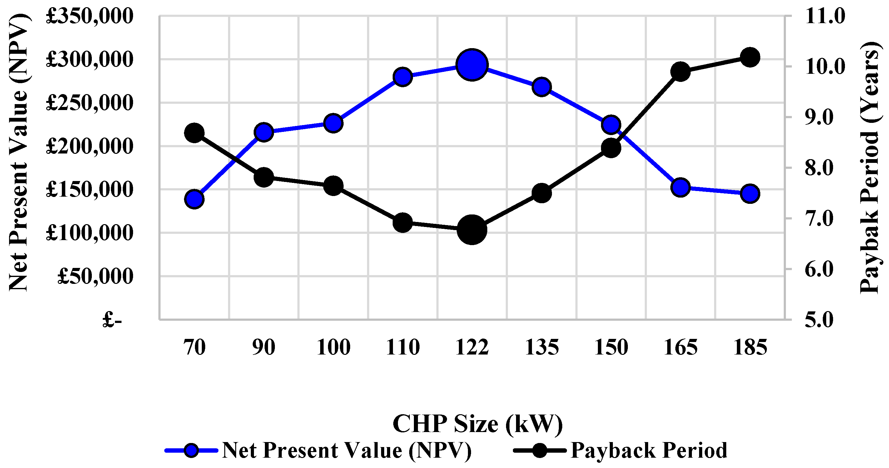
2.5. Optimum Sizing of CHP

A careful deliberation is required when the optimal size of the CHP is determined. A typical practice is to size a CHP system as per the buildings thermal base load [24]. Such a system may operate at 100% capacity, but due to its smaller size, it will not fully meet the buildings electrical and thermal demands, and therefore, the building will remain heavily dependent on grid and boilers for meeting its electricity and thermal demands. Secondly, the higher cost of grid electricity and boilers gas consumption will certainly make such a smaller CHP system an unfeasible solution, resulting in a longer payback period of the project. However, under certain situations, such a CHP system may be successful, e.g., where the difference between the building’s base load and the peak load is small [25].
On the other hand, higher savings could be achieved using an optimum sized electricity led or thermal led modulating CHP. It is understood that offsetting the grid electricity in a higher proportion will generate higher financial and environmental savings, and this could be achieved using an electricity led CHP system, which will modulate as per the buildings electricity demand. However, at the same time, the excess heat generation should be minimal and the Quality Index (QI) of CHP systems remains above 105. Generally, the modulating CHP systems are programmed to stop when the building load is less than 50% output of the CHP system. For example, if the building load is 70 kW and the CHP’s output capacity is 200 kW, CHP will stop until the load increases to 100 kW (i.e., 50% of the CHP capacity). Such oversized CHP systems running on the part load, will require frequent maintenance and will result in reduced financial savings. On the other hand, a system that is too small (undersized) will result in a longer payback period of the project. Therefore, a careful study of the building’s hourly thermal and electricity demand profiles is indispensable, and only a validated CHP sizing model should be used for sizing a CHP system. Poorly or incorrectly sized systems will not perform optimally and will lead to a complete loss of investment [26].
CHP Sizing has been performed using the LSBU CHP model. This model was developed by Amber [12] as a part of his PhD studies. The model has been validated against different models and is capable of sizing CHP for a single or multiple buildings [27]. Although it allows testing of multiple operating strategies, only mixed heat and electricity led CHP with minimum excess heat generation has been considered in this study. The following criteria for the optimum size of the CHP has been set:
  • CHP should have minimum 5500 running hours operating between 75% and 100% load;
  • higher net present value (NPV);
  • higher internal rate of return (IRR), %; and
  • lower payback period.
Table 1 shows the values of different parameters that have been fed into the LSBU CHP model for obtaining results. Tariffs, climate change levy (CCL) rates and value added tax (VAT) rates for electricity and gas usage were available from the electricity and gas bills, whereas CHP related cost figures were received from ENERG, a leading CHP supplier in the UK. Project duration, inflation rate and weighted average cost of capital (WACC) rate were used after consultation with the university’s project management team.

3. Results

Using the real hourly thermal demand profiles and electrical demand profiles for the mixed control strategy of the CHP, the LSBU CHP model generated results for nine different sizes of CHP ranging from 70 kW to 185 kW. Table 2 shows the results obtained from the LSBU model.
Figure 13 shows the plot of payback period and NPV for different sizes of CHP investigated for this building.
The results clearly suggest that 122-kW CHP is an optimum size for McLaren House which will not only generate higher financial savings, but also result in a lower payback period, i.e., 6.8 years. The 122-kW CHP will offset grid electricity by 77.5%, whereas it will result in an increase in the site’s gas consumption by 25.3%. The CHP system will also reduce the site’s carbon emissions by 281 tonnes of CO2.

4. Sensitivity Analysis

4.1. Effect of Estimated Energy Demand Profiles on the CHP System’s Sizing and Economics

As discussed earlier, the economics of a CHP plant strongly depend on its optimum sizing, where optimum sizing is strongly dependent on the accuracy of the buildings hourly energy consumption profiles. Use of estimated or incorrect energy profiles could lead to an undersized or oversized CHP system and could affect its economics. The LSBU model was run seven times by feeding hourly demand profiles, having an error range from −30% to +30% with an interval of 10%. Table 3 shows the results generated by the LSBU CHP model.
It is apparent that if the hourly demand profiles have a −20% error, the model suggests that the optimum size is 110 kW, which would result in an undersized CHP system. Similarly, with a +20% error, the model suggests an oversized CHP size of 135 kW. Another interesting result that could be drawn from this analysis is that under-sizing of CHP is not as bad as over-sizing. It could be seen if the hourly profiles have +20% error, the results could be misleading as is obvious from Table 3. Table 3 shows that installing 135-kW CHP will result in a NPV of only £40,558 with an IRR of 7%. However, this size of CHP will generate a NPV of £268,150 with an IRR of 15%, as shown earlier in Table 2. This clearly demonstrates how important the accuracy of hourly energy profiles is for the optimum sizing of CHP.

4.2. Effect of Variation in Electricity and Fuel Prices

The financial risk is considered as one of the main barriers for investing in energy-efficient technologies [28]. One of such possible risks is uncertainty of electricity and gas prices [29]. Wickart and Madlener [30] found that, under higher price volatility levels, a CHP system offers more profit than a conventional generation plant.
To investigate the effect of such future fluctuations in the electricity and fuel prices, the LSBU model performs a sensitivity analysis of the payback period by considering the future variations in the electricity and fuel prices in the range between −10% and +40%. The results are presented in Table 4 and Figure 14.
It is apparent that with increasing electricity and fuel prices, the payback period of the CHP system decreases, and vice versa.

4.3. Significant Parameters (Monte Carlo Analysis)

In order to identify the most influential parameter, the LSBU CHP model was used to run a Monte Carlo simulation for 10,000 iterations and calculate the values of two statistical parameters, i.e., coefficient of correlation (R) and coefficient of determination (R2). Both “R” and “R2” demonstrate degree of the relationship between a variable and the payback period of the project. Table 5 shows the results. It is apparent that day-time electricity price has the strongest but negative relationship with the payback period (R = −0.87), i.e., if it increases in future, the payback period will decrease. The fuel price has a positive but not strong relationship with the payback period (R = 0.33).
The LSBU CHP model was used to generate a histogram of the payback period, as shown in Figure 15, and calculate the cumulative probability for the payback period. It is apparent that there is 92% probability that the optimum size of CHP, i.e., 122 kW identified in this study, will have a payback period shorter than seven years. This type of analysis helps the higher management in the decision-making process.

5. Conclusions

To highlight the significance of the optimum sizing of a CHP system, a detailed economic and environmental assessment of a CHP system has been performed using the LSBU CHP model for a student residence hall building located in central London, the UK. The following conclusions have been drawn from this study.
  • Availability of real hourly electricity and thermal demand profiles is crucial for the optimum sizing of a CHP system.
  • CHP sizing based on estimated energy profiles, monthly energy consumption figures or based on the existing boilers capacity may result in an undersized or oversized CHP system.
  • Weather normalization of real hourly energy consumption data is mandatory for finding the optimum size of CHP.
  • Under-sizing of a CHP system is better than over-sizing.
  • Variation in electricity and fuel prices could affect the project’s economics.
  • Increase in electricity price will decrease the payback period of the project and will strengthen its economics over its life period.
  • Electricity price has the strongest relationship (R2 = 0.75) with the project’s payback period.
  • Variation in CCL tax, VAT tax and O&M price has the minimal effect on the project’s economics.
  • An optimum sized CHP is a suitable solution for student residence hall type buildings and could generate considerable financial and environmental savings for the university sector.
The results of this study clearly indicate that university buildings, such as student residence halls that occupy nearly 24% space of a typical university campus, offer a good opportunity for the installation of CHP systems. However, the sizing of a CHP system is crucial and must be optimized carefully in order to achieve higher financial and environmental benefits. While a CHP system is sized, real hourly electricity and thermal demand data must be used. This real hourly data could be managed through the installation of smart meters in the university buildings. Normalization of this hourly energy consumption data is mandatory for the calculation of an optimum sized CHP system. CHP optimization exercise must be performed using a validated CHP sizing model. This study has clearly shown that universities that have had installed CHP systems have positively managed to reduce their carbon emissions. Yet only 41% universities in the UK have had installed CHP systems. One of the major challenges is the lack of support from the universities’ higher management. If the higher management of universities support such clean energy production initiatives, the university sector of the UK could certainly achieve its carbon reduction targets and could play a considerable role towards a greener environment.

Author Contributions

Conceptualization, K.P.A. and A.R.D.; Methodology, K.P.A. and N.I.R.; Software, K.P.A.; Investigation, K.P.A.; Data Curation, K.P.A.; Formal Analysis, K.P.A., R.A. and M.A.; Writing-Original Draft Preparation, K.P.A., N.I.R., R.A. and M.A.; Writing-Review & Editing, K.P.A., A.R.D., R.A.; Supervision, K.P.A. and A.R.D.

Acknowledgments

Authors would like to thank Anuj Saush (Sustainability Manager at London South Bank University) for providing their energy consumption data. We would also like to thank Mark Kelly (Project development Engineer, ENERG) for providing technical and operational performance data of their UK CHP installations and for guiding us on the capital cost calculations.

Conflicts of Interest

The authors declare no conflicts of interest.

Abbreviation

BMSBuilding Management System
CCLClimate Change Levy
CHPCombined Heat and Power
CRCCarbon Reduction Commitment
IRRInternal Rate of Return
kWKilowatts
kWhKilo Watts Hour
LSBULondon South Bank University
NPVNet Present Value
O&MOperations and Maintenance
UKUnited Kingdom
WACCWeighted Average Cost of Capital

References

  1. Higher Education Funding Council for England (HEFCE). Carbon Reduction Target and Strategy for Higher Education in England. Available online: http://www.hefce.ac.uk/pubs/year/2010/201001/ (accessed on 11 September 2012).
  2. Higher Education Statistics Agency. Environmental Information, Estates Management Statistics Tables. Available online: https://www.hesa.ac.uk/index.php?option=com_heicontacts&Itemid=87 (accessed on 10 October 2016).
  3. Amber, K.P.; Parkin, J. Barriers to the uptake of combined heat and power technology in the UK higher education sector. Int. J. Sustain. Energy 2015, 34, 406–416. [Google Scholar] [CrossRef]
  4. Raine, R.D.; Sharifi, V.N.; Swithenbank, J. Optimisation of combined heat and power production for buildings using heat storage. Energy Convers. Manag. 2014, 87, 164–174. [Google Scholar] [CrossRef]
  5. Amber, K.P.; Day, T.; Ratyal, N.I.; Kiani, A.K.; Ahmad, R. Techno, Economic and Environmental Assessment of a Combined Heat and Power (CHP) System—A Case Study for a University Campus. Energies 2018, 11, 1133. [Google Scholar] [CrossRef]
  6. Chen, H.; Xu, J.; Xiao, Y.; Qi, Z.; Xu, G.; Yang, Y. An Improved Heating System with Waste Pressure Utilization in a Combined Heat and Power Unit. Energies 2018, 11, 1515. [Google Scholar] [CrossRef]
  7. Franco, A.; Versace, M. Optimum sizing and operational strategy of CHP plant for district heating based on the use of composite indicators. Energy 2017, 124, 258–271. [Google Scholar] [CrossRef]
  8. Amber, K.P.; Aslam, M.W.; Mahmood, A.; Kousar, A.; Younis, M.Y.; Akbar, B.; Chaudhary, G.Q.; Hussain, S.K. Energy Consumption Forecasting for University Sector Buildings. Energies 2017, 10, 1579. [Google Scholar] [CrossRef]
  9. Wu, Q.; Ren, H.; Gao, W.; Ren, J. Multi-criteria assessment of building combined heat and power systems located in different climate zones: Japan-China comparison. Energy 2016, 103, 502–512. [Google Scholar] [CrossRef]
  10. Amber, K.P.; Aslam, W.; Bashir, M.A. Development of a Typical Hourly Electricity Consumption Profile for Student Residence Halls Based on Central Tendency Method. Nucleus 2016, 53, 14–25. [Google Scholar]
  11. Athawale, R.; Felder, F.A.; Goldman, L.A. Do Combined Heat and Power plants perform? Case study of publicly funded projects in New York. Energy Policy 2016, 97, 618–627. [Google Scholar] [CrossRef]
  12. NewEnCo, Benefits of CHP. Available online: http://www.newenco.co.uk/combined-heat-power/benefits-of-chp (accessed on 13 November 2012).
  13. Amber, K.P. Development of a Combined Heat and Power Sizing Model for the Higher Education Sector of the United Kingdom. Ph.D. Thesis, London South Bank University, London, UK, 2013. [Google Scholar]
  14. Taljan, G.; Verbič, G.; Pantoš, M.; Sakulin, M.; Fickert, L. Optimal sizing of biomass-fired Organic Rankine Cycle CHP system with heat storage. Renew. Energy 2012, 41, 29–38. [Google Scholar] [CrossRef]
  15. Ren, H.; Gao, W.; Ruan, Y. Optimal sizing for residential CHP system. Appl. Therm. Eng. 2008, 28, 514–523. [Google Scholar] [CrossRef]
  16. Amber, K.P.; Aslam, M.W.; Ikram, F.; Kousar, A.; Ali, H.M.; Akram, N.; Afzal, K.; Mushtaq, H. Heating and Cooling Degree-Days Maps of Pakistan. Energies 2018, 11, 94. [Google Scholar] [CrossRef]
  17. Büyükalaca, O.; Bulut, H.; Yılmaz, T. Analysis of variable-base heating and cooling degree-days for Turkey. Appl. Energy 2001, 69, 269–283. [Google Scholar] [CrossRef] [Green Version]
  18. Martinaitis, V.; Bieksa, D.; Miseviciute, V. Degree-days for the exergy analysis of buildings. Energy Build. 2010, 42, 1063–1069. [Google Scholar] [CrossRef]
  19. Soldo, B. Forecasting natural gas consumption. Appl. Energy 2012, 92, 26–37. [Google Scholar] [CrossRef]
  20. Olofsson, T.; Andersson, S.; Östin, R. Energy load predictions for buildings based on a total demand perspective. Energy Build. 1998, 28, 109–116. [Google Scholar] [CrossRef]
  21. Olofsson, T.; Andersson, T. Long-term energy demand predictions based on short-term measured data. Energy Build. 2001, 33, 85–91. [Google Scholar]
  22. Heating and Cooling Degree Days. Available online: http://www.degreedays.net/ (accessed on 21 November 2012).
  23. Charter Institute of Building Services Engineers (CIBSE). TM41 Degree Days: Theory and Application, 2008. Available online: http://www.ihs.com/info/st/e/info4education.aspx (accessed on 22 September 2014).
  24. Salem, R.; Bahadori-Jahromi, A.; Mylona, A.; Godfrey, P.; Cook, D. Comparison and evaluation of the potential energy, carbon emissions, and financial impacts from the incorporation of CHP and CCHP systems in existing UK hotel buildings. Energies 2018, 11, 1219. [Google Scholar] [CrossRef]
  25. Yu, D.; Meng, Y.; Yan, G.; Mu, G.; Li, D.; Blond, S.L. Sizing Combined Heat and Power Units and Domestic Building Energy Cost Optimisation. Energies 2017, 10, 771. [Google Scholar] [CrossRef]
  26. ENERG—A Guide to CHP Unit Sizing. Available online: http://www.energ-group.com/combined-heat-and-power/cogeneration/essential-guide-to-chp/ (accessed on 21 November 2012).
  27. Amber, K.P.; Dunn, A.; Parkin, J.; Day, A.R. Development of a combined heat and power sizing model for higher education buildings in the United Kingdom. Energy Build. 2018, 172, 537–553. [Google Scholar] [CrossRef]
  28. Maurovich-Horvat, L.; Rocha, P.; Siddiqui, A.S. Optimal operation of combined heat and power under uncertainty and risk aversion. Energy Build. 2016, 110, 415–425. [Google Scholar] [CrossRef] [Green Version]
  29. Teymouri-Hamzehkolaei, F.; Sattari, S. Technical and economic feasibility study of using Micro CHP in the different climate zones of Iran. Energy 2011, 36, 4790–4798. [Google Scholar] [CrossRef]
  30. Wickart, M.; Madlener, R. Optimal technology choice and investment timing: A stochastic model of industrial cogeneration vs. heat-only production. Energy Econ. 2007, 29, 934–952. [Google Scholar] [CrossRef]
Figure 1. Energy consumption in residential and non-residential buildings [2].
Sustainability 10 02069 g001
Figure 2. Yearly variation in the Combined Heat and Power (CHP) generation and the number of universities that install the CHP [2].
Sustainability 10 02069 g002
Figure 3. Front view of McLaren House.
Sustainability 10 02069 g003
Figure 4. Monthly electricity and gas consumption of McLaren House.
Sustainability 10 02069 g004
Figure 5. Relationship between the last five years average monthly HDDs and the monthly gas consumption.
Sustainability 10 02069 g005
Figure 6. Comparison between actual monthly and normalized gas consumption for the year 2011.
Sustainability 10 02069 g006
Figure 7. Relationship between the last five years average monthly HDDs and the monthly electricity consumption.
Sustainability 10 02069 g007
Figure 8. Comparison between the actual monthly and normalized gas consumption for the year 2011.
Sustainability 10 02069 g008
Figure 9. Hourly electricity consumption profile for a winter month.
Sustainability 10 02069 g009
Figure 10. Hourly electricity consumption profile for a summer month.
Sustainability 10 02069 g010
Figure 11. Hourly thermal demand profile for a winter month.
Sustainability 10 02069 g011
Figure 12. Hourly thermal demand profile for a summer month.
Sustainability 10 02069 g012
Figure 13. Optimization curves for the optimum CHP Sizing.
Sustainability 10 02069 g013
Figure 14. Sensitivity analysis of payback period.
Sustainability 10 02069 g014
Figure 15. Histogram of Monte Carlo simulation results for the payback period.
Sustainability 10 02069 g015
Table 1. Values of input parameters.
ParameterValue
Electricity day tariff7.875 p/kWh
Electricity night tariff4.801 p/kWh
Electricity fixed charges£12,000
Natural gas tariff2.375 p/kWh
CCL charges on electricity usage0.524 p/kWh
CCL charges on gas usage0.182 p/kWh
Boiler’s efficiency78%
VAT charge@20%
CRC cost£12/t/CO2
CO2 emission factor for electricity0.541 kg/kWh
CO2 emission factor for natural gas0.194 kg/kWh
O&M cost per kWh at 100% load£0.01/kWh
O&M cost per kWh at 100% load£0.012/kWh
O&M cost per kWh at 100% load£0.013/kWh
Weighted average cost of capital (WACC)5%
Annual inflation rate5%
Project Life 15 years
CHP asset cost£200,000
Infrastructure Cost50% of CHP cost
Switch room modification10% of CHP cost
G59 Application fee2% of CHP cost
In-house project management fee5% of CHP cost
Out-sourced project management fee5% of CHP cost
BMS connection fee2% of CHP cost
Other costs5% of CHP cost
Contractor’s preliminaries5% of CHP cost
Project contingency7% of CHP cost
Table 2. Optimum Sizing of CHP for McLaren House.
CHP Size (kW)Total Running HoursRunning Hours >75%Payback Period, YearsNPV (£)IRR (%)CO2 Savings
t/CO2
Reduction in Grid Electricity (%)Increase in Gas Consumption (%)QI
70866886368.7138,8881218053.2619.33125
90863580047.8215,8491423865.0120.97127
100855169467.6226,3001524469.1323.60125
110863565056.9279,7351627274.0623.72128
122851258966.8293,5741728177.4825.30128
135797553877.5268,1501528277.9825.64129
150726342938.4224,4761327176.5325.95129
165628132939.9152,2671024571.8525.72125
1855903249210.2145,1531025271.1824.18129
Table 3. Effect of incorrect demand profiles on the optimum sizing of CHP.
Error, %Optimum
CHP Size, kW
Total Running HoursRunning Hours >75%Pay- Back Period, YearsNPV (£)IRR (%)CO2 Saving
t/CO2
Reduction in Grid Electricity (%)Increase in Gas Consumption (%)QI
−20110787351194.9507,1202422677.9125.54128
−15110827356435.2458,4152224278.1725.36128
−10110847458965.6401,7542025577.2824.93128
0122851258966.77293,574172817725128
+10122863564388.7169,9021229974.4324.16128
+151358626619210.6104,443932276.7124.87129
+201358635638212.640,558732975.0524.27129
Table 4. Effect of variation in electricity and fuel prices on the payback period of CHP.
−10%Gas Cost Now10%20%30%40%
−10%7.88.79.811.112.814.9
Electricity cost now6.26.77.48.29.210.4
10%5.05.45.96.57.17.8
20%4.14.54.85.25.76.2
30%3.53.74.04.34.65.0
40%3.03.23.43.63.94.2
50%2.52.72.93.13.33.5
Table 5. Variables and their relationship with the payback period of CHP.
VariableRR2
Fuel price0.330.10856
Day electricity price−0.870.75490
Night electricity price−0.170.02838
CRC allowance price−0.160.02716
VAT, % for electricity−0.020.00053
VAT, % for fuel0.010.00005
O & M Cost−0.010.00003
CCL rate for fuel0.040.00148
CCL rate for electricity −0.060.00348

