Identifying Core Parts in Complex Mechanical Product for Change Management and Sustainable Design

Abstract

Changes in customer needs are unavoidable during the design process of complex mechanical products, and may bring severely negative impacts on product design, such as extra costs and delays. One of the effective ways to prevent and reduce these negative impacts is to evaluate and manage the core parts of the product. Therefore, in this paper, a modified Dempster-Shafer (D-S) evidential approach is proposed for identifying the core parts. Firstly, an undirected weighted network model is constructed to systematically describe the product structure. Secondly, a modified D-S evidential approach is proposed to systematically and scientifically evaluate the core parts, which takes into account the degree of the nodes, the weights of the nodes, the positions of the nodes, and the global information of the network. Finally, the evaluation of the core parts of a wind turbine is carried out to illustrate the effectiveness of the proposed method in the paper. The results show that the modified D-S evidential approach achieves better performance regarding the evaluation of core parts than the node degree centrality measure, node betweenness centrality measure, and node closeness centrality measure.

1. Introduction

With the slowdown in global economic growth, different strategies have been proposed in recent years, such as “Industry 4.0”, “Made in China 2025”, etc. These strategies point out that the key to affecting the level of manufacturing is the competitiveness of the equipment manufacturing industry [1,2]. There are many ways to improve the competitiveness of the equipment manufacturing industry. On the one hand, optimizing material flow and applying lean products in the production process can reduce the company’s production costs and help obtain competitive prevalence [3,4]. On the other hand, improving the design capability of the equipment manufacturing industry is the key issue for improving the company’s production level and obtaining competitive advantages [5]. This paper focuses on how to improve the design capability of the equipment manufacturing industry. In fact, the vast majority of products in the equipment manufacturing industry are complex mechanical products, such as large ships, weapons, and high-speed trains [6]. Under this background, trying to improve the ability to design complex mechanical products is not only an issue that companies must face when meeting market challenges, but also a key approach to improving national core competitiveness [7].

Changes in customer needs often occur in the development of complex mechanical products, and are difficult to avoid [8,9]. On the one hand, changes in customer needs are regarded as an important source of product innovation and sustainable design [10,11,12]. On the other hand, changes in customer needs may bring severely negative impacts on product design, such as extra costs and delays, even an avalanche [13,14]. Generally, a need change is firstly mapped to a change of one part or some parts. In addition, due to the large number of parts and the complicated relationship between parts, a change occurring in one part may cause a series of changes in other parts that are connected to it, or even spread farther, eventually resulting in an avalanche effect. So, effectively dealing with changes in customer needs, accelerating the speed of the change response, and improving the agility of product development have become the main ways to improve the competitiveness of enterprises in this area [15].

The existing research studies on changes in customer needs and engineering change management mainly focus on change propagation [16,17,18], change impact [19,20], and change control [21,22]. There is no study of engineering change prevention. However, it is of great significance to carry out engineering change prevention for reducing the change impact, the market response time, and the product design costs. In the research studies on engineering change prevention, it is important to identify the exact core parts that control the propagation direction and the impact scope of the changes. Identifying core parts and focusing attention on them are important contents regarding change management, which is of great significance for reducing the impact of changes and preventing the avalanche effect. In this study, a core part is referred to as a part that plays a decisive role in change propagation speed and scope when changes in customer needs occur. Based on those analyses, which are oriented to the changes in customer needs, it is necessary to design an effective method that can be used to evaluate the core parts of complex mechanical products when changes in customer needs occur.

In recent years, studies have shown that systems with hierarchical structures and complex internal relations can be modeled by complex network theory [23,24,25]. For example, complex networks were used to deal with intertwined problems among the logistics network, information network, and financial network. Combining the product characteristics, a structure network model is constructed based on the complex network theory [26,27,28]. On the basis of the model, the evaluation of the core parts of a complex mechanical product can be regarded as the evaluation of core nodes in the network model. In general, node centrality is used to evaluate the influence degree of a node on other nodes, in which the bigger the node centrality, the more critical the node.

The node centrality assessment methods can be divided into four categories in the existing research studies.

(1) The node centrality assessment methods that consider the neighbors number of the node. Chen et al. proposed a semi-local centrality measure to evaluate the performance by using the spreading rate and the number of infected nodes [29]. Chen etc. proposed a local ranking algorithm named ‘cluster rank’, which takes into account not only the number of neighbors and the neighbors’ influences, but also the clustering coefficient [30]. Kitsak et al. proposed a K-shell decomposition method, which provides a route for an optimal design of efficient dissemination strategies [31]. Among them, the semi-local centrality and cluster rank algorithm are local assessment methods of node centrality, which cannot make a global assessment of node centrality, and easily lead to inaccurate assessment results. The K-shell decomposition method cannot effectively evaluate the node centrality for a complex network with a large number of nodes.

(2) The node centrality assessment methods depend on the path. Dolev et al. presented algorithms for computing the Routing Betweenness Centrality (RBC) of all the individual vertices in the network, and algorithms for computing the RBC of a given group of vertices [32]. Freeman developed three methods for each concept: one absolute and one relative measure of the centrality of a position in a network, and one relenting the degree of centralization of the entire network [33]. Brandes proposed a betweenness centrality method, which substantially increased the range of networks for which centrality analysis is feasible [34]. Most of these methods are global optimization algorithms. The main disadvantage of these methods is their high time complexity.

(3) The node centrality assessment methods based on eigenvectors. Bonacich et al. proved that there is a necessary addition to the concepts of the degree, closeness, and betweenness centrality, as distinguished by Freeman [35]. Brin and Page addressed building a practical large-scale system that could exploit the additional information present in hypertext [36]. Lempel and Moran proved that the stochastic approach for link-structure analysis (SALSA) is equivalent to a weighted in-degree analysis of the link-structure of World Wide Web sub graphs, making it computationally more efficient than the mutual reinforcement approach [37]. Chen et al. put forward the understanding model of complex product systems (CoPS) from the viewpoint of the width and depth of technology and the technology development model of CoPS [38]. These methods require multiple iterative convergences, and most of are better for a directed network.

(4) The node centrality assessment methods based on node removal and shrinkage. Dangalchev proposed a new characteristic (residual closeness), which can measure the network resistance that is presented [39]. Li et al. used the sum of the reciprocal of all the geodesics between a pair of disconnected actors caused by deleting an actor (set) to characterize the extent to which the network has been destroyed [40]. Tan et al. proposed a node contraction method of evaluation of node importance in complex networks based on a new evaluation criterion [41]. These methods are mostly used in power networks, internet, transportation networks, etc.

Based on the above analyses, it is found that the factors affecting the node centrality include three aspects: the number of the node neighbors, the strength of the node, and the position of nodes in the network. However, in addition to the above deficiencies, the main shortage of the existing methods is that most of the methods evaluate node centrality from a single point of view, which resulting in an inability to achieve a systematic and accurate assessment of node centrality. In order to solve these issues, a modified D-S evidential approach is proposed in this study. The effectiveness of the proposed method is verified by comparing it with other three methods of node centrality evaluation. Moreover, the case study indicates that the proposed method can be used to accurately evaluate the core parts.

The rest part of this paper is organized as follows. An undirected weighted network model is constructed in Section 2. Section 3 proposes a modified D-S evidential approach for core nodes evaluation. Section 4 is a case study; in this section, the evaluation of core parts of a wind turbine is used to verify the proposed approach. Finally, conclusions are represented.

2. The Construction of a Network Model

The expression of product structure is the basis of identifying core parts. Due to complex mechanical products containing a large number of parts and there being complex correlations between different parts, complex network theory was used to model the product structure. The constructed network model can systematically and quantitatively express the product structure [28]. In the network model, the parts are defined as nodes, while the relationship between parts are defined as edges, and the strength of the edges is used to express the network weight. Therefore, the network model $G_s$ is defined as follows:

$$G_s=\left(V,E,W\right)$$

(1)

$V=\left\{v_i,i=1,2,\dots ,n\right\}$ is the set of nodes, where $v_i$ is the $i$-th part of a complex mechanical product; $E=\left\{e_{ij},i,j=1,2,3,\dots ,n,i\ne j\right\}$ is the set of edges, where $e_{ij}$ denotes the relationship between $v_i$ and $v_j$; and $W=\left\{w_{ij},i,j=1,2,3,\dots ,n,i\ne j\right\}$ is the strength of edge weights, where $w_{ij}$ denotes the strength of $e_{ij}$.

The determination of weights is a key step for constructing a network model. In this study, the weights of the network model are determined by considering functional and structural aspects. The comprehensive weight can be calculated as follows:

$$w_{ij}=\alpha w_{ij}^f+\beta w_{ij}^s$$

(2)

where $\alpha$ and $\beta$ correspond to the weights of $w_{ij}^f$ and $w_{ij}^s$, respectively. $w_{ij}^f$ is the total functional load value that the $v_j$ can bear relative to $v_i$.$w_{ij}^s$ denotes the structural correlation strength between $v_i$ and $v_j$.

The weight $w_{ij}^f$ is determined by the functional load, and the value is calculated as follows:

$$w_{ij}^f={\displaystyle \sum _{h=1}^H\frac{f_h}{F_h}}$$

(3)

where $f_h$ is the functional load that $v_j$ can bear for the realization of function $h$, and $F_h$ is the total functional capacity.

The weight $w_{ij}^s$ is determined by the structural constraints, such as size constraints, shape constraints, etc., and it can be calculated as follows:

$$w_{ij}^s={\displaystyle \sum _{l=1}^L{w}_{ij-l}^s}$$

(4)

where $w_{ij-l}^s$ denotes the correlation strength of the $l$-th kind of structural correlations. $L$ represents the total number of types of structural correlations.

It should be noted that the greater the correlation strength between two nodes, the greater the weight of the node.

3. A Modified D-S Evidential Approach for Core Nodes Evaluation

A core part is refers to a part that plays a decisive role in change propagation speed and scope when changes occur. Determining whether a part is a core part is based on its influence on other parts. Correspondingly, the identification of core parts refers to identifying those nodes that have an important influence for the network model. Due to the node centrality indicating the influence degree of the node on other nodes, the identification of the influence nodes can be seen as the calculation of the node centrality. The greater the node centrality, the greater the influence degree of this node on the other nodes in network.

The classical D-S evidential method is a node centrality calculation method in the complex network theory, which is often used to deal with uncertain problems [4]. The classical D-S evidential method has considered the number of the node neighbors and the strength of the node for node centrality calculation; however, this method ignores the position of the node and the global structure of the network. Therefore, in order to systematically and scientifically evaluate the node centrality, a modified D-S evidential approach is proposed in this study.

The modified approach is embodied in two aspects. Firstly, the position information of the node is considered by introducing the semi-local centrality measure. According to the definition and calculation formula of the semi-local centrality method [29], the semi-local centrality method reflects the position information of the node in the network by considering both the nearest and the next nearest neighbors. In this study, the value of node centrality is calculated by the D-S evidential approach, and is further processed by the idea of the semi-local centrality method. Secondly, the global information of the network is considered by adding the calculation of the shortest path. In this study, the basic probability assignments (BPAs) are calculated not only based on the node degree, but also based on the shortest path. In short, the calculation results of the modified D-S evidential approach not only reflect the degree and weight of the node, they also reflect the position information and global information of the network, which makes the results more systematic and accurate.

This section has two parts: Section 3.1 includes a definition of all the parameters involved in the proposed method, and Section 3.2 is the detailed calculation process of the modified D-S evidential approach.

3.1. Parameters Definition

All of the parameters that are involved in the modified D-S evidential are defined in this section, as shown in

Table 1. The description of parameters. BPAs: basic probability assignments.

Notations	Illustrate
$\eta$	A frame of discernment
$high$/$low$	The evaluation indices for the degree of a node as “a core node” and “a non-core node”
$m_{ki}\left(high\right)$/$m_{ki}\left(low\right)$	The probabilities of “high” and “low” influence for the degree of node $v_i$
${\alpha }_i$	The corrected parameter of node degree calculation
$k_i$	The degree of node $v_i$
$k_{\max }$/$k_{\min }$	The maximum and minimum values of a node degree in the network
$m_{di}\left(high\right)$/$m_{di}\left(low\right)$	The probabilities of “high” and “low” influence for the shortest path between $v_i$ and other nodes
$d_{ij}$	The shortest path between $v_i$ and $v_j$
$d_{i\max }$/$d_{i\min }$	The maximum and minimum values of the shortest path between $v_i$ and other nodes
$\Gamma \left(i\right)$	The set of nodes that connected (nearest neighbors) with $v_i$
$p\left(k_i\right)$	The degree distribution
$H\left(j\right)$	The set of nodes that is a degree is lower than $k_i$
$M_k\left(i\right)$/$M_d\left(i\right)$	The BPAs of the node $v_i$ with respect to the degree and shortest path
$M\left(i\right)$	Integration of the BPAs of $v_i$
$m_i\left(high\right)$/$m_i\left(low\right)$	The integration probabilities of “high” and “low” influence for $v_i$
$m_i\left(\theta \right)$	The probability of “high” or “low”
$M_i\left(high\right)$/$M_i\left(low\right)$	The final probabilities of “high” and “low” of $v_i$
$\sigma$/$\delta$	Constants
$ENC\left(i\right)$	The evidential node centrality of $v_i$
$ENC{\left(i\right)}_{\min }$	The minimum value of evidential node centrality
$NC\left(i\right)$	The node centrality of $v_i$
$\Gamma \left(i\right)$	The set of nodes that is next nearest neighbor of $v_i$

. The table contains the notations of all of the parameters, as well as a specific description of the parameters.

3.2. The Calculation Process of Node Centrality

A frame of discernment $\eta$ is defined as follows:

$$\eta =\left(high,low\right)$$

(5)

The basic probability assignment (BPA) for each node is given as follows.

$$m_{ki}\left(high\right)={\alpha }_i\frac{\left|k_i-k_{\min }\right|}{\left(k_{\max }+\sigma \right)-\left(k_{\min }-\sigma \right)}$$

(6)

$$m_{ki}\left(low\right)=\left(1-{\alpha }_i\right)\frac{\left|k_i-k_{\max }\right|}{\left(k_{\max }+\sigma \right)-\left(k_{\min }-\sigma \right)}$$

(7)

$$m_{di}\left(high\right)=\frac{1}{n}{\displaystyle \sum _{j=1}^n{m}_{dij}\left(high\right)=\frac{1}{n}{\displaystyle \sum _{j=1}^n\frac{\left|d_{ij}-d_{i\min }\right|}{\left(d_{i\max }+\xi \right)-\left(d_{i\min }-\xi \right)}}}$$

(8)

$$m_{di}\left(low\right)=\frac{1}{n}{\displaystyle \sum _{j=1}^n{m}_{dij}\left(low\right)}=\frac{1}{n}{\displaystyle \sum _{j=1}^n\frac{\left|d_{i\max }-d_{ij}\right|}{\left(d_{i\max }+\xi \right)-\left(d_{i\min }-\xi \right)}}$$

(9)

$$k_i={\displaystyle \sum _{j\in \Gamma \left(i\right)}{w}_{ij}}$$

(10)

Suppose node $v_i$ with degree $k_i$ follows a degree distribution $p\left(k_i\right)$. Thus, ${\alpha }_i$ is defined as follows:

$${\alpha }_i={\displaystyle \sum _{{\rm H}\left(j\right)\le k_i}p\left(j\right)}$$

(11)

The BPAs of the $v_i$ are calculated based on the degree and shortest path, as follows:

$$M_k\left(i\right)=\left(m_{ki}\left(high\right),m_{ki}\left(low\right),1-m_{ki}\left(high\right)-m_{ki}\left(low\right)\right)$$

(12)

$$M_d\left(i\right)=\left(m_{di}\left(high\right),m_{di}\left(low\right),1-m_{di}\left(high\right)-m_{di}\left(low\right)\right)$$

(13)

Integration of the BPAs of $v_i$ is calculated as follows:

$$M\left(i\right)=\left(m_i\left(high\right),m_i\left(low\right),m_i\left(\theta \right)\right)=M_k\left(i\right)\oplus M_d\left(i\right)$$

(14)

Generally, in the Equation (13), let $m_i\left(\theta \right)$ assign to $m_i\left(high\right)$ and $m_i\left(low\right)$ averagely, then:

$$M_i\left(high\right)=m_i\left(high\right)+\frac{1}{2m_i\left(\theta \right)}$$

(15)

$$M_i\left(low\right)=m_i\left(low\right)+\frac{1}{2m_i\left(\theta \right)}$$

(16)

Therefore, the node centrality of $v_i$ is shown as follows:

$$ENC\left(i\right)=M_i\left(high\right)-M_i\left(low\right)=m_i\left(high\right)-m_i\left(low\right)$$

(17)

In order to ensure that $ENC\left(i\right)$ is a positive number, the numerical treatment and normalization are represented as follows:

$$EN{C}^{\prime }\left(i\right)=\frac{\left|ENC{\left(i\right)}_{\min }\right|+ENC\left(i\right)}{{\displaystyle \sum _{i=1}^n\left\{\left|ENC{\left(i\right)}_{\min }\right|+ENC\left(i\right)\right\}}}$$

(18)

According to the computing idea of a semi-local centrality measure, the value of $EN{C}^{\prime }\left(i\right)$ is further optimized, and the value of $NC\left(i\right)$ is obtained. The value of $NC\left(i\right)$ is equal to the sum of $EN{C}^{\prime }\left(i\right)$, the nearest and the next nearest neighbors’ ENC’ of node $v_i$.

$NC\left(i\right)$ is calculated as follows:

$$NC\left(i\right)=EN{C}^{\prime }\left(i\right)+{\displaystyle \sum _{j\in \Gamma \left(i\right)}EN{C}^{\prime }\left(j\right)}+{\displaystyle \sum _{s\in \mathsf{\Upsilon }\left(i\right)}EN{C}^{\prime }\left(s\right)}$$

(19)

The higher the value of $NC\left(i\right)$, the bigger the node centrality of $v_i$. In other words, the parts with bigger values of $NC\left(i\right)$ are regarded as core parts.

4. Case Study

The evaluation of core parts of a wind turbine is used to verify the proposed method. Specifically, the purpose of this study is to verify that the modified proposed has a positive effect on reducing the impact of changes in customer needs on wind turbine design, preventing the change avalanche, decreasing the design delay, and reducing extra costs.

In this section, firstly, the structure of the wind turbine is described and transformed into a network structure based on complex network theory. Secondly, the node centrality is calculated with the proposed method; this means that the core parts are evaluated, too. Finally, the proposed method and calculation results are discussed by comparing them with the existing methods.

4.1. The Construction of the Network Model

According to the research in Section 2, the structure of the wind turbine is described and transformed as a network model by using complex network theory. In the network model, the parts of the wind turbine are defined as nodes, the relationships between the parts are defined as the edges, and the strength of the edges constitute the network weight.

By considering the representation of this study, the main parts of the wind turbine (as listed in

Table 2. The weights of the influencing factors.

	${\mathit{w}}_1$	${\mathit{w}}_2$
Factors	Functional	structural
Weight	0.4	0.6

) are selected.

According to the research in Section 2 and combining with the characteristics of wind turbines, the weights of the structure of a wind turbine are determined by considering both the functional and structural elements. Due to the influence of different factors, the weights of the factors evaluated by experts and calculated based on the entropy method are enumerated in Table 2.

For the calculation of the weights, firstly, 10 designers and experts took these two factors (functional and structural) as the evaluation index of the relationship between parts, and then judged the correlation strength between the parts using linguistic variables. The relationship strength of the linguistic variables are divided into six levels, including very strong, strong, middle, weak, very weak, and no. The value of these six levels are 0.9 (very strong), 0.7 (strong), 0.5 (middle), 0.3 (weak), 0.1 (very weak), and 0 (no), respectively. Secondly, on this basis, the edge weights are calculated according to Equations (2)–(4). The calculation results are shown in

Table 3. The weights of the network model.

Parts		${\mathit{v}}_1$	${\mathit{v}}_2$	${\mathit{v}}_3$	${\mathit{v}}_4$	${\mathit{v}}_5$	…	${\mathit{v}}_{26}$	${\mathit{v}}_{27}$	${\mathit{v}}_{28}$	${\mathit{v}}_{29}$	${\mathit{v}}_{30}$
Blade	$v_1$	—	0.788				…		0.198
Rotor hub	$v_2$	0.788	—			0.113	…	0.033	0.221	0.113
Rotor bearing	$v_3$			—			…	0.032	0.2	0.032
Gearbox casing	$v_4$				—		…
Stator winder	$v_5$		0.113			—	…
⁞	⁞	⁞	⁞	⁞	⁞	⁞	⁞	⁞	⁞	⁞	⁞	⁞
Cabinet tower	$v_{26}$		0.033	0.032			…	—		0.835
Yaw drive	$v_{27}$	0.198	0.221	0.2			…		—
Tower arrester bracket	$v_{28}$		0.113	0.032			…	0.835		—
Warning circuit	$v_{29}$						…				—	0.815
Microcomputer controller	$v_{30}$						…				0.815	—

. Based on this, the network model is represented by UCINET 6, which systematically and intuitively depicts the structure of the wind turbine (as shown in Figure 1).

4.2. The Evaluation of Core Parts

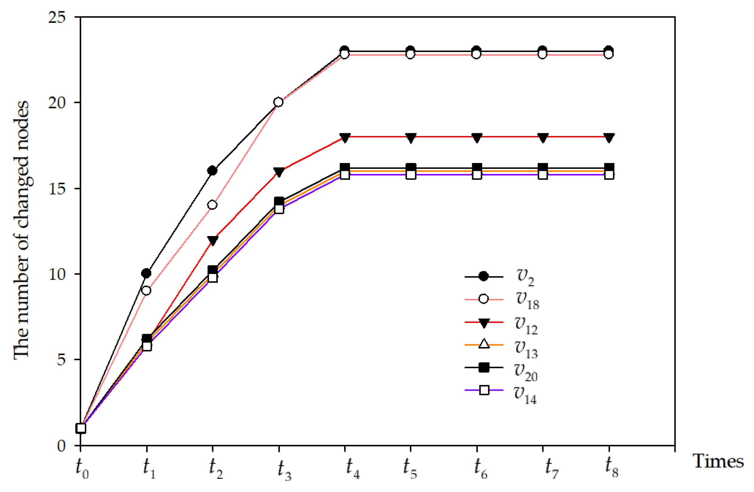
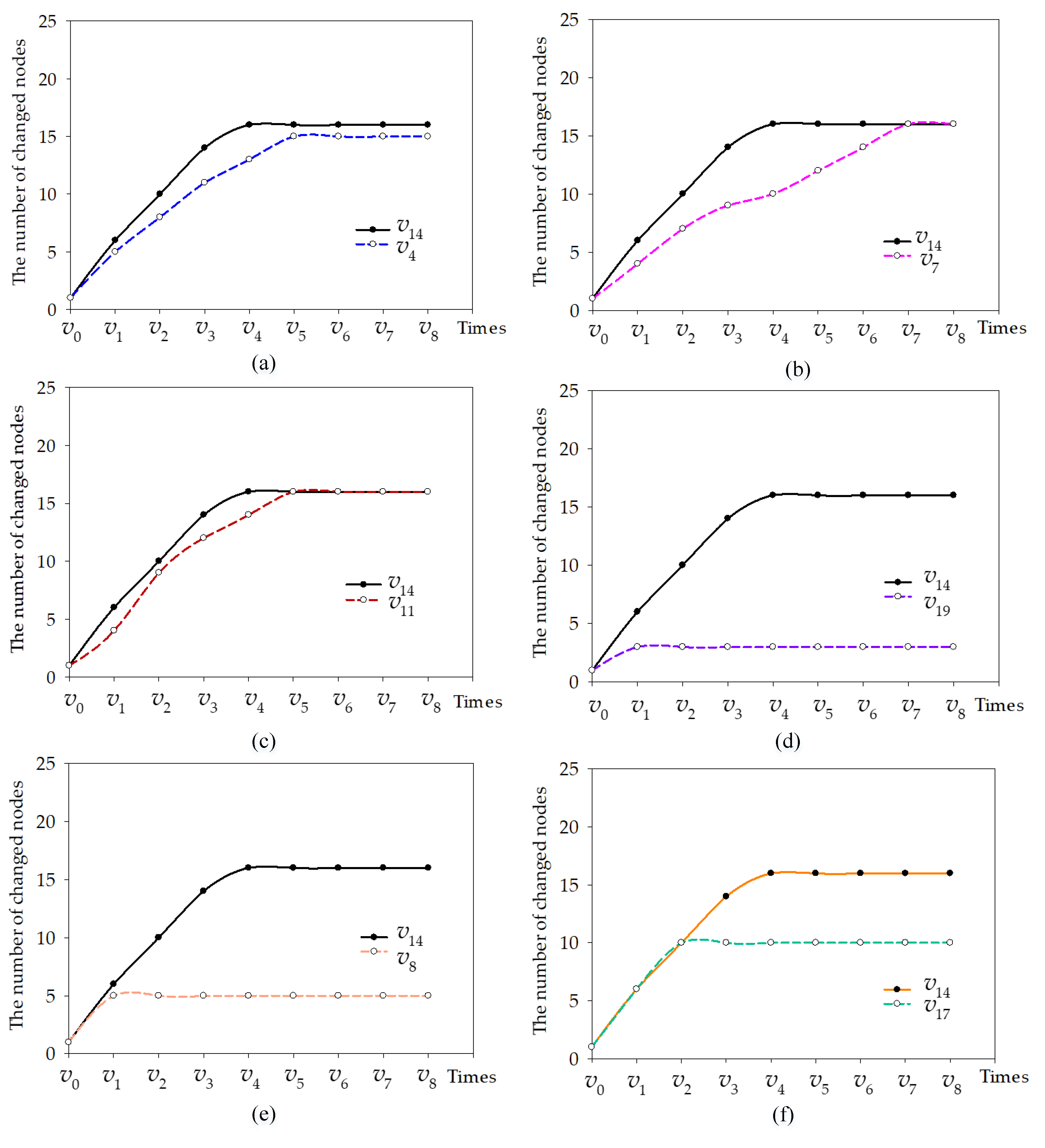
Based on the constructed network model, the $NC\left(i\right)$ values of the nodes are calculated by using the modified D-S evidential approach according to Equations (4)–(18). The calculated results are shown in Figure 2.

As shown in Figure 2, node $v_2$ (Rotor hub) has the largest value of node centrality in the network model. From this, it can be seen that the node $v_2$ is a core node in the structure network model of the wind turbine. When node $v_2$ changes, it will cause other nodes to change in the structure network model, which will cause the greatest impact on the model. In addition, other nodes with greater centrality include node $v_{18}$ (Nacelle support), $v_{12}$ (Deflector), $v_{13}$ (Rotor lock insert), $v_{20}$ (Nacelle frame), and $v_{14}$ (Blade bearing), where the corresponding values of $NC$ are 151.954, 147.603, 136.178, 134.664, and 127.803. These nodes can be seen as core nodes in the network model. Correspondingly, rotor hub, nacelle support, deflector, rotor lock insert, nacelle frame, and blade bearing are core parts of the wind turbine. It can be seen that the larger the node centrality of the node, the higher influence of the node.

In order to reduce the impact of changes, as well as decrease the market response time and design costs, the change buffer of core parts should be added during the wind turbine design process. Specifically, in the design process of the wind turbine, the core parts of the wind turbine should have a certain design margin as a change buffer. The change is amplified when the change of a part that is caused by changes exceeds its change buffer; otherwise, the change is absorbed.

4.3. Discussion

In order to verify the effectiveness and the advantages of the proposed method, the analysis and verification of the calculation results are carried out from two aspects. On the one hand, the validity of the proposed method is verified by analyzing and discussing the results obtained in this paper. On the other hand, the results obtained in this paper are compared with the results obtained by other methods to verify the advantages of the proposed method. Due to differences in the calculations, the results cannot be directly compared and discussed. Therefore, in order to verify the advantages and effectiveness of the proposed method, in this paper, the SI model of a complex network was introduced.

The SI model is used to describe the change propagation process in the network. It can also be understood as the description of the nodes’ state (unchanged node and changed node) in the network at each moment of the change propagation process. The SI model is described as follows.

Each node in the SI model is allowed to have two states, namely the unchanged node and the changed node. The change propagation process refers to the process in which a changed node causes a change in an unchanged node. The change propagation capability is the probability that the changed node causes a change in the other unchanged nodes; that is, the change propagation rate can be used to reflect the change propagation capability of a node. The greater the change propagation rate of a node, the more changes it will cause.

The change propagation rate between two nodes is defined:

$${\lambda }_{ij}={\left(\frac{w_{ij}}{w_M}\right)}^{\alpha },\alpha >0$$

(20)

where ${\lambda }_{ij}$ denotes the propagation rate from the changed node $v_j$ to the unchanged node $v_i$. $w_M$ denotes the maximum weight in the structure network.

The change propagation rate of node $v_i$ can be calculated as follows:

$${\lambda }_i=1-{\displaystyle \prod _{j\in V_t}\left(1-{\lambda }_{ij}\right)}$$

(21)

where $V_t$ denotes the set of changed nodes in the neighbor of the node $v_i$.

In addition, the change propagation threshold ${\lambda }_c$ of structure network is defined as follows:

$${\lambda }_c=\frac{1}{{\Lambda }_m}$$

(22)

where ${\Lambda }_m$ represents the feature vector value of the parts’ relationship matrix.

In this paper, the SI model was used to verify the proposed method through the change propagation process in the network.

Firstly, the calculation results of the modified D-S evidential are analyzed and discussed.

The top 20% nodes of node centrality value in the network are selected for analyzing; that is, $v_2$, $v_{18}$, $v_{12}$, $v_{13}$, $v_{20}$, and $v_{14}$ are selected for analyzing. These nodes are selected as the initially changed nodes and input into the SI model. In addition, the change propagation rates at each time under different initially changed nodes are calculated, and then, the number of changed nodes at each time can be determined. Based on this, the change propagation process is simulated. The propagation and impact of the initial change nodes on the network are analyzed based on the simulated results. The comparison of the change propagation influence of different initially changed nodes ($v_2$, $v_{18}$, $v_{12}$, $v_{13}$, $v_{20}$, and $v_{14}$) is shown in Figure 3.

As shown in Figure 3, the abscissa represent the times of change in the propagation process. The ordinate represents the number of changed nodes, which is used to describe the change propagation capability of the initially changed node in the structure network of a wind turbine. The change propagation process of these six nodes as initially changed nodes are shown in Figure 3. The six curves represents the number of changed nodes at different times of different initially changed nodes. $t_0$ is the initial time at which a change occurs. The change propagation is completed at $t_8$.

As shown in Figure 3, node $v_2$, as the initially changed node in the structure network of a wind turbine, has the fastest propagation speed compared to others nodes as initially changed nodes. Moreover, node $v_2$ causes the most changes to the nodes in the network (23 nodes are changed in the network). Therefore, node $v_2$ is considered to have the strongest change propagation capability. The change propagation speed of node $v_{18}$ as the initially changed node is slower than the change propagation speed of node $v_2$; meanwhile, node $v_{18}$ also causes the most changes to the nodes in the network (the same as node $v_2$). The change propagation speed of node $v_{12}$ as the initially changed node is slower than that of node $v_2$ and node $v_{18}$, and is faster than node $v_{13}$, node $v_{20}$, and node $v_{14}$. In addition, the number of node changes causing by node $v_{12}$ is less than that of node $v_2$ and node $v_{18}$, and is more than node $v_{13}$, node $v_{20}$, and node $v_{14}$. Finally, the change propagation speed and changed nodes are the same as those of node $v_{13}$, node $v_{20}$, and node $v_{14}$ as initially changed nodes, eventually causing 16 nodes to be changed in the network.

The compared results are in agreement with the results of the proposed method. From the analyses results, it can be seen that the nodes identified by the modified D-S evidential approach have a greater impact on the network. In other words, the proposed method is effective.

Secondly, in order to verify the advantages of the proposed method, the proposed method was compared with other node centrality evaluation methods.

In this section, the degree centrality (DC), the betweenness centrality (BC), and the closeness centrality (CC) [42] are compared with the proposed method in this study. Firstly, we calculate the value of the DC, BC, and CC of nodes in the network model of the wind turbine. Secondly, the top 20% nodes regarding node centrality value, as calculated by these methods, are selected for analysis. Some nodes are selected as the initially changed nodes and input into the SI model. In addition, the change propagation rates at each time under different initially changed nodes are calculated, and then, the number of changed nodes at each time can be determined. Based on this, the proposed method that is verified has advantages over the other methods.

The DC, BC, and CC of wind turbine parts are calculated, respectively. The calculation results are shown in

Table 4. The degree centrality (DC), betweenness centrality (BC), and closeness centrality (CC) of nodes in a structure network model.

No.	DC	BC	CC	No.	DC	BC	CC	No.	DC	BC	CC
$v_1$	6.603	0.006	0.004	$v_{11}$	6.642	0.006	0.005	$v_{21}$	6.316	0.027	0.003
$v_2$	9.794	0.091	0.003	$v_{12}$	10.007	0.110	0.004	$v_{22}$	6.529	0.056	0.004
$v_3$	5.536	0.049	0.004	$v_{13}$	10.081	0.081	0.005	$v_{23}$	3.972	0.051	0.003
$v_4$	6.433	0.008	0.005	$v_{14}$	8.109	0.033	0.003	$v_{24}$	5.513	0.029	0.004
$v_5$	3.541	0.000	0.003	$v_{15}$	7.911	0.031	0.005	$v_{25}$	2.796	0.037	0.003
$v_6$	4.581	0.042	0.003	$v_{16}$	7.720	0.024	0.004	$v_{26}$	4.279	0.011	0.002
$v_7$	8.134	0.043	0.005	$v_{17}$	8.547	0.162	0.008	$v_{27}$	6.177	0.035	0.003
$v_8$	8.636	0.101	0.004	$v_{18}$	9.647	0.104	0.008	$v_{28}$	4.615	0.014	0.002
$v_9$	7.401	0.026	0.004	$v_{19}$	6.296	0.027	0.005	$v_{29}$	2.519	0	0.003
$v_{10}$	3.744	0.005	0.002	$v_{20}$	9.503	0.096	0.004	$v_{30}$	3.259	0.037	0.003

.

As shown in Table 4, the degree centrality, betweenness centrality, and closeness centrality of nodes in the network model are calculated. It can be seen that the node with the largest degree centrality is node $v_{13}$, which is followed by nodes $v_{12}$, $v_2$, $v_{18}$, $v_{20}$, and $v_8$. Meanwhile, the node with the largest betweenness centrality is node $v_{17}$, followed by nodes $v_{12}$, $v_{18}$, $v_3$, $v_{20}$, and $v_2$. In additional, the node with largest closeness centrality is node $v_{18}$, followed by node $v_{17}$, $v_{11}$, $v_{19}$, $v_7$, and $v_4$. Based on the calculation results, the ranking of core nodes in a network with the modified D-S evidential approach, DC, BC, and CC are obtained. The top 20% of nodes are selected for sorting, which are shown in

Table 5. The ranking of core nodes in the network model by different methods.

Rank	The Proposed Method	DC	BC	CC
1	$v_2$	$v_{13}$	$v_{17}$	$v_{18}$
2	$v_{18}$	$v_{12}$	$v_{12}$	$v_{17}$
3	$v_{12}$	$v_2$	$v_{18}$	$v_{11}$
4	$v_{13}$	$v_{18}$	$v_8$	$v_{19}$
5	$v_{20}$	$v_{20}$	$v_{20}$	$v_7$
6	$v_{14}$	$v_8$	$v_2$	$v_4$

.

Obviously, the calculation results regarding node centrality with these four methods are different; however, the advantages of the four methods cannot be directly compared and discussed. For this reason, the SI model is introduced.

According to the ranking results of the modified D-S evidential approach and DC (as shown in Table 5), it can be seen that there are seven nodes ($v_2,v_{18},v_{12},v_{13},v_{20},v_{14},v_8$) in the two rankings. Due to the effectiveness of the modified D-S evidential approach being proven (as shown in Figure 3), the rank of the change propagation capability of these nodes ($v_2,v_{18},v_{12},v_{13},v_{20},v_{14}$) is obtained; that is, $v_2>v_{18}>v_{12}>v_{13}>v_{20}>v_{14}$. Therefore, the node $v_{14}$ (the weakest change propagation capability in ranking of the modified D-S evidential approach) is selected to compare with node $v_8$ (node $v_8$ has not been analyzed). According to the ranking results of the modified D-S evidential approach and BC, it can be seen that there are eight nodes ($v_2,v_{18},v_{12},v_{13},v_{20},v_{14},v_8,v_{17}$) in the two rankings. Based on the existing analysis, similarly, the node $v_{14}$ is selected to compare with node $v_{17}$ (node $v_{17}$ has not been analyzed). According to the ranking results of the modified D-S evidential approach and BC, it can be seen that there are 11 nodes ($v_2,v_{18},v_{12},v_{13},v_{20},v_{14},v_{17},v_{11},v_{19},v_7,v_4$) in the two rankings. Based on the existing analysis, similarly, node $v_{14}$ is selected to compare with node $v_{11}$, node $v_{19}$, node $v_7$, and $v_4$ (these nodes have not been analyzed).

Therefore, the propagation influence of six groups of nodes are compared (as shown in Figure 4). These nodes are selected as the initially changed nodes, and are input into the SI model. After that, the change propagation process is simulated. The propagation and impact of the initial change nodes on the network are analyzed based on the simulated results.

The simulation results are shown in Figure 4. As shown in Figure 4, the abscissa represents the times of change propagation. The ordinate represents the number of changed nodes, which is used to describe the change impact of the initially changed node in the wind turbine structure network.

In Figure 4b,c, it can be seen that the node $v_{14}$ propagates more quickly than node $v_7$ and $v_{11}$. The propagation scopes corresponding to node $v_{14}$, node $v_7$ and node $v_{11}$ are the same. In Figure 4a,d–f, it can be seen that node $v_{14}$ propagates more quickly and infects more largely than $v_4$, $v_{19}$ $v_8$, and $v_{17}$. However, considering the change propagation speed and change impact scope, it is easy to see and know whether the comprehensive change propagation capability of node $v_{14}$ is greater than that of nodes $v_4$, $v_7$, $v_8$, $v_{11}$, $v_{17}$, and $v_{19}$.

Moreover, the two nodes with the largest node centrality calculated by the four methods are selected as the initially changed nodes and are input into the SI model. The propagation and impact of the initially changed nodes are analyzed based on the simulated results, as shown in Figure 5.

In Figure 5, the four curves represents the number of changed nodes of the four methods at different times. $t_0$ is the initial time when the change occurs. The change propagation is completed at $t_7$. It should be noted that when the change propagation is completed, the propagation scopes corresponding to the proposed method and betweenness centrality are same. However, considering the change propagation speed and change impact scope, it can be noticed that the proposed method is better than the other three methods.

Based on the above analysis, it can be seen that the nodes identified by the modified D-S evidential approach have a greater impact on the network. In other words, the proposed method has advantages over other methods.

In summary, the change of these core nodes is the root cause of avalanche transmission. Controlling and managing core nodes are the core of change management. It is an important measure to reduce the impact of customer’s needs changes, and thus decrease the market response time and design costs. Therefore, identifying core parts and giving large buffers of core parts are both effective measures to reduce the change influence.

5. Concluding Remarks

Meeting customer needs is an integral part of the sustainable design of complex mechanical products. In order to reduce the impact of changing customer needs and prevent an avalanche, it is of great importance to identify the core parts that have great impact in product design. Complex network theory is used for network modeling and the evaluation of core parts in the study. In evaluation, the core parts are transformed to calculate the centrality of the nodes. An undirected weighted network model is established that is used to systematically describe the structure of the products. Based on the constructed network, the modified D-S evidential approach is proposed, which is used to calculate the node centrality. By introducing the semi-local centrality measure and adding the calculation of the shortest path, the calculation results of the modified D-S evidential approach not only reflect the degree and weight of the node, they also reflect the position information and global information of the network, which makes the results more systematic and accurate. Moreover, it has been proven that the modified D-S evidential is effective. Furthermore, the study has proved that the nodes identified by the modified D-S evidential approach have a greater change propagation capability and a greater change impact on the network. In other words, the proposed method has advantages over other methods.

In addition, the redundant design of core parts is the research direction for the further exploration oriented toward changes in customer needs and engineering.

References

1. Akgün, A.E.; Keskin, H.; Byrne, J.C. Complex adaptive systems theory and firm product innovativeness. J. Eng. Technol. Manag. 2014, 31, 21–42. [Google Scholar] [CrossRef]
2. Wang, F.J.; Shen, S.D. Comparison and enlightenment of equipment manufacturing in the United States, Japan and South Korea. J. Huazhong Norm. Univ. (Hum. Soc. Sci.) 2012, 51, 38–46. [Google Scholar]
3. Krolczyk, J.B.; Krolczyk, G.M.; Legutko, S.; Napiorkowski, J.; Hloch, S.; Foltys, J.; Tama, E. Material flow optimization-a case study in automotive industry. Tehnicki Vjesnik/Tech. Gaz. 2015, 22, 1447–1456. [Google Scholar]
4. Lehocká, D.; Hlavatý, I.; Hloch, S. Rationalization of material flow in production of semitrailer frame for automotive industry. Tehnički Vjesnik 2016, 23, 1215–1220. [Google Scholar]
5. Fernandes, J.; Henriques, E.; Silva, A. A method for imprecision management in complex product development. Res. Eng. Des. 2014, 25, 309–324. [Google Scholar] [CrossRef]
6. Chen, Y.; Hu, A.Q.; Hu, X. Evaluation method for node importance in communication networks. J. China Inst. Commun. 2004, 25, 129–134. [Google Scholar]
7. Dan, B.; Guo, L.F.; Jing, Y.G. Maintance service method of customer need-driven for large and complex products. Comput. Integr. Manuf. Syst. 2012, 18, 888–895. [Google Scholar]
8. Ma, S.H.; Jiang, Z.L.; Liu, W.P. Design Property Network-Based Change Propagation Prediction Approach for Mechanical Product Development. Chin. J. Mech. Eng. 2017, 30, 676–688. [Google Scholar] [CrossRef]
9. Yang, F. Searching Model of Change Propagation Paths for Mechanical Product Based on Characteristic Linkage Network. J. Mech. Eng. 2011, 47, 97–106. [Google Scholar] [CrossRef]
10. Baxter, J.; Gram-Hanssen, I.; Askham, C.; Hansen, I.J.B.; Rubach, S. Exploring sustainability metrics for redesigned consumer products. J. Clean. Prod. 2018, 190, 128–136. [Google Scholar] [CrossRef]
11. Cheng, H.; Chu, X.N. A network-based assessment approach for change impacts on complex product. J. Intell. Manuf. 2012, 23, 1419–1431. [Google Scholar] [CrossRef]
12. Dyllick, T.; Rost, Z. Towards true product sustainability. J. Clean. Prod. 2017, 162, 346–360. [Google Scholar] [CrossRef] [Green Version]
13. Kim, S.; Moon, S.K. Sustainable platform identification for product family design. J. Clean. Prod. 2017, 143, 567–581. [Google Scholar] [CrossRef]
14. Tang, D.B.; Xu, R.H.; Tang, J.C. Analysis of Engineering Change Impacts Based on Design Structure Matrix. J. Mech. Eng. 2010, 46, 154–161. [Google Scholar] [CrossRef]
15. Gong, Z.W.; Mo, R.; Yang, H.C. Engineering changes based on hub nodes of product development network. Comput. Integr. Manuf. Syst. 2012, 18, 40–46. [Google Scholar]
16. Clarkson, P.J.; Simons, C.; Eckert, C. Predicting change propagation in complex design. J. Mech. Des. 2004, 136, 52–68. [Google Scholar] [CrossRef]
17. Cohen, T.; Navathe, S.B.; Fulton, R.E. C-FAR, change favorable representation. Comput. Aided Des. 2000, 32, 321–338. [Google Scholar] [CrossRef]
18. Koh, E.C.Y.; Caldwell, N.H.M.; Clarkson, P.J. A method to assess the effects of engineering change propagation. Res. Eng. Des. 2012, 23, 329–351. [Google Scholar] [CrossRef]
19. Li, Y.; Wei, Z.; Ma, Y. A shortest path method for sequential change propagations in complex engineering design processes. AI EDAM 2016, 30, 107–121. [Google Scholar] [CrossRef]
20. Morkos, B.; Shankar, P.; Summers, J.D. Predicting requirement change propagation, using higher order design structure matrices: An industry case study. J. Eng. Des. 2012, 23, 905–926. [Google Scholar] [CrossRef]
21. Tang, D.B.; Yin, L.L.; Ullah, I. Workload-based change propagation analysis in engineering design. Concurr. Eng. 2016, 24, 83–109. [Google Scholar] [CrossRef]
22. Yang, F.; Duan, G.J. Developing a parameter linkage-based method for searching change propagation paths. Res. Eng Des. 2012, 23, 353–372. [Google Scholar] [CrossRef]
23. Cruz, J.M.; Nagurney, A.; Wakolbinger, T. Financial engineering of the integration of global supply chain networks and social networks with risk management. Nav. Res. Log. 2006, 53, 674–696. [Google Scholar] [CrossRef]
24. Hu, C.L.; Rong, Z.J.; Chen, K.S. Research on process model of product design based on path searching. Comput. Integr. Manuf. Syst. 2013, 19, 293–299. [Google Scholar]
25. Wakolbinger, T.; Nagurney, A. Dynamic supernetworks for the integration of social networks and supply chains with electronic commerce: Modeling and analysis of buyer-seller relationships with computations. Netnomics 2004, 6, 153–185. [Google Scholar] [CrossRef]
26. Keivanpour, S.; Kadi, D.A. An integrated approach to analysis and modeling of End of Life phase of the complex products. IFAC-PapersOnLine 2016, 49, 1892–1897. [Google Scholar] [CrossRef]
27. Li, Y.P.; Wang, Z.T.; Zhang, L. Function Module Partition for Complex Products and Systems Based on Weighted and Directed Complex Networks. J. Mech. Des. 2017, 139, 021101. [Google Scholar] [CrossRef]
28. Zhang, N.; Yang, Y.; Zheng, Y.J.; Su, J.F. Module partition of complex mechanical products based on weighted complex networks. J. Intell. Manuf. 2017, 6, 1–26. [Google Scholar] [CrossRef]
29. Chen, D.; Lü, L.; Shang, M.S. Identifying influential nodes in complex networks. Phys. A 2012, 391, 1777–1787. [Google Scholar] [CrossRef] [Green Version]
30. Chen, D.B.; Gao, H.; Lu, L.Y. Identifying Influential Nodes in Large-Scale Directed Networks: The Role of Clustering. PLoS ONE 2013, 8, e77455. [Google Scholar] [CrossRef] [PubMed]
31. Kitsak, M.; Gallos, L.K.; Havlin, S. Identification of influential spreaders in complex networks. Nat. Phys. 2010, 6, 888–893. [Google Scholar] [CrossRef] [Green Version]
32. Dolev, S.; Elovici, Y.; Puzis, R. Routing betweenness centrality. J. ACM 2010, 57, 1–27. [Google Scholar] [CrossRef]
33. Freeman, L.C. Centrality in social networks conceptual clarification. Soc. Netw. 1978, 1, 215–239. [Google Scholar] [CrossRef] [Green Version]
34. Brandes, U. A Faster Algorithm for Betweenness Centrality. J. Math. Sociol. 2001, 25, 163–177. [Google Scholar] [CrossRef]
35. Bonacich, P.; Lloyd, P. Eigenvector-like measures of centrality for asymmetric relations. Soc. Netw. 2001, 23, 191–201. [Google Scholar] [CrossRef] [Green Version]
36. Brin, S.; Page, L. The anatomy of a large-scale hypertextual Web search engine. Comput. Netw. 2012, 56, 3825–3833. [Google Scholar] [CrossRef]
37. Lempel, R.; Moran, S. The stochastic approach for link-structure analysis (SALSA) and the TKC effect. Comput. Netw. 2000, 33, 387–401. [Google Scholar] [CrossRef] [Green Version]
38. Chen, J.; Huang, J.Z.; Tong, L. Technology development model of complex product system. RD Manag. 2004, 16, 65–70. [Google Scholar]
39. Dangalchev, C. Residual closeness in networks. Phys. A 2006, 365, 556–564. [Google Scholar] [CrossRef]
40. Li, P.X.; Ren, Y.Q.; Xi, Y.M. An importance measure of actors (set) within a network. Syst. Eng. 2004, 22, 13–20. [Google Scholar]
41. Tan, Y.J.; Wu, J.; Deng, H.Z. Evaluation method for node importance based on node contraction in complex networks. Syst. Eng. Theory Pract. 2016, 11, 79–83. [Google Scholar]
42. Opsahl, T.; Agneessens, F.; Skvoretz, J. Node centrality in weighted networks: Generalizing degree and shortest paths. Soc. Netw. 2010, 32, 245–251. [Google Scholar] [CrossRef]
Figure 1. The structure network model of the wind turbine.
Sustainability 10 04480 g001
Figure 2. The N C ( i ) of nodes in network model.
Sustainability 10 04480 g002
Figure 3. The comparison of propagation influence of different initially changed nodes.
Sustainability 10 04480 g003
Figure 4. Comparison of the propagation influence of different initially changed nodes.
Sustainability 10 04480 g004
Figure 5. The influence of customer’s needs changes with the four methods.
Sustainability 10 04480 g005