Endogenous or Exogenous? Examining Trans-Boundary Air Pollution by Using the Air Quality Index (AQI): A Case Study of 30 Provinces and Autonomous Regions in China

Abstract

China is experiencing severe environmental degradation, particularly air pollution. To explore whether air pollutants are spatially correlated (i.e., trans-boundary effects) and to analyse the main contributing factors, this research investigates the annual concentration of the Air Quality Index (AQI) and 13 polluting sectors in 30 provinces and autonomous regions across China. Factor analysis, the linear regression model and the spatial auto-regression (SAR) model are employed to analyse the latest data in 2014. Several important findings are derived. Firstly, the global Moran’s I test reveals that the AQI of China shows a distinct positive spatial correlation. The local Moran’s I test shows that significant high–high AQI agglomeration regions are found around the Beijing–Tianjin–Hebei area and the regions of low–low AQI agglomeration all locate in south China, including Yunnan, Guangxi and Fujian. Secondly, the effectiveness of the SAR model is much better than that of the linear regression model, with a significantly improved R-squared value from 0.287 to 0.705. A given region’s AQI will rise by 0.793% if the AQI of its ambient region increases by 1%. Thirdly, car ownership, steel output, coke output, coal consumption, built-up area, diesel consumption and electric power output contribute most to air pollution according to AQI, whereas fuel oil consumption, caustic soda output and crude oil consumption are inconsiderably accountable in raising AQI. Fourthly, the air quality in Beijing and Tianjin is under great exogenous influence from nearby regions, such as Hebei’s air pollution, and cross-boundary and joint efforts must be committed by the Beijing–Tianjin–Hebei region in order to control air pollution.

1. Introduction

With its rapid economic development and acceleration of industrialisation and modernisation, China needs enormous energy sources and metal and chemical products to sustain its rapidly growing socio-economic demands [1,2,3]. Large amounts of harmful gases are emitted by polluting sectors through massive industrial production, and these gases lead to severe air pollution [4,5,6]. Grossman et al. [7] demonstrated that the relationship between economic development and environmental quality generally follows the environmental Kuznets curve. This curve indicates the presence of a general process where environmental quality and economic development interact with each other. Economic development at initial stages leads to environmental degradations, which in turn inhibits economic development and causes it to slow down. Committed efforts are needed to control pollution and improve the ecological environment. As the environment recovers, the economy regains its high development speed. Considering this hypothesis, scholars have widely discussed the relationship between the economy and the environment. China has progressed remarkably in terms of economic development but at the cost of environmental degradation. Ma and Zhang [8] stated that the economic development level of China remains far from the inflection point of environmental quality; in the future, economic development in China will intensify environmental pollution.

Although the state and local governments have established various measures to prevent and control pollution, pollution incidents occur occasionally [9,10]. The air quality is worsening and the haze is thickening owing to extensive production; secondary industry occupies significantly high weights in the national economy; economic development speed exceeds the carrying capacities of resources and environment; and there is an imbalance between environment protection and economic development and environmental improvement neglecting the effect of pollution [11]. In January 2013, excessive and large-scale haze hit China, affecting more than 8 million citizens; it was considered the worst air pollution incident in China since the last century [12]. Emission of air pollutants and environmental pollution harm the health of citizens in most areas of China and reduce their life expectancy [13,14]. With the improvement of living standards in China, awareness about environment protection and the willingness to appeal for a better environment have increased. Air pollution has received increasing attention from the public in China [15].

The air quality index (AQI) was launched in China in 2012 to quantify air quality for monitoring and evaluating air pollution by the Ministry of Environmental Protection of People’s Republic of China. AQI is a dimensionless index that differs from the previously used air pollution index, which considers only SO₂, NO₂ and PM₁₀. AQI is calculated according to the new ambient air quality standard (GB3095-2012). The six pollutants included in AQI calculation are SO₂, NO₂, PM₁₀, PM_2.5, O₃ and CO [16,17]. The subindex of each pollutant is calculated firstly according to the graded concentration limits standard (

Table 1. Air quality pollutants graded concentration limits standard.

IAQI	Air Pollutants Concentration Limits
	SO2	SO2	NO2	NO2-	PM10	CO	CO	O3	O3	PM2.5
	−24 h AV	−1 h AV	−24 h AV	1 h AV	−24 h AV	−24 h AV	−1 h AV	−1 h AV	−8 h MAV	−24 h AV
0	0	0	0	0	0	0	0	0	0	0
50	50	150	40	100	50	2	5	160	100	35
100	150	500	80	200	150	4	10	200	160	75
150	475	650	180	700	250	14	35	300	215	115
200	800	800	280	1200	350	24	60	400	265	150
300	1600		565	2340	420	36	90	800	800	250
400	2100		750	3090	500	48	120	1000		350
500	2620		940	3840	600	60	150	1200		500

Note: The unit is μg/m³. AV and MAV refer to average and moving average, respectively.

), marked as IAQI_p.

$$IAQ{I}_p=\frac{IAQ{I}_{Hp}-IAQ{I}_{Lp}}{B{P}_{Hp}-B{P}_{Lp}}\left(C_p-B{P}_{Lp}\right)+IAQ{I}_{Lp}$$

(1)

In Equation (1), IAQI_p refers to the subindex of pollutant p; C_p is the concentration of pollutant p; BP_Hp is the high value of pollutant concentration limit close to C_p; BP_Lp is the low value of pollutant concentration limit close to C_p; IAQI_Hp and IAQI_Lp are the corresponding air quality subindex to BP_Hp and BP_Lp respectively. Then, AQI is derived by the rule of AQI = max{IAQI₁, IAQI₂, ···, IAQI_n}. High AQI indicates severe and aggregative air pollution that will not only affect the outdoor activities of people but also harm their health. Wang et al. [18] pointed out that the release of China’s AQI standards is later than that of developed countries; the evaluation results of China’s SO₂-1 h average and PM_2.5-24 h average at the low concentration interval of AQI < 200 are low and loose, compared with America and Hong Kong. In addition, China’s AQI real-time report has a certain degree of lag in the average sliding time of particulate matter and ozone, compared to foreign countries. This indicates continuous improvement is needed. However, China’s AQI has distinct advantages and characteristics relative to those of other countries. For example, China’s AQI includes more types of pollutants compared with that of the United States. In fact, China’s AQI contains the largest number of pollutants in the world [18], so it can make most comprehensive consideration of various air pollutants. Meanwhile, the calculation method of AQI of China makes it more objectively reflect the characteristics of air pollution and citizens’ perception of air quality [19]. All these advantages ensure that AQI is an effective indicator for studying air pollution.

AQI has been widely studied in China by using different methods, emphasised areas and perspectives. Some scholars conducted their studies from a local area perspective. For instance, Li et al. [20] investigated general air quality, AQI level, seasonal characteristics and distribution of main pollutants in 13 cities within the Beijing–Tianjin–Hebei metropolitan region. Results showed that in 2015, the overall average AQI of these 13 cities was 98, and the air pollution was most serious in winter, with an average AQI of 122. Liu et al. [21] evaluated AQI, SO₂, NO₂, PM₁₀, PM_2.5, O₃ and CO recorded by 10 air-quality automatic monitoring stations in Dalian from June to August in 2015; this research found that the value of AQI would rise during rush hour and would decrease on rainy days; the AQI in Dalian had a significant correlation with PM_2.5 and PM₁₀. Zhan et al. [22] used the inverse distance weighting method and geographic information system spatial analysis to analyse the AQI data observed by the air quality automatic monitoring station in Wuhan in the first half of 2013; this study concluded that the AQI in Wuhan showed a distinct temporal and spatial characteristic. From January to June, the AQI in Wuhan gradually decreased, the high-AQI area in the central city gradually shrank; the value of AQI in north Wuhan was higher than that in the south; and the relevance between pollution indicators and AQI from high to low was PM_2.5, CO, SO₂, NO₂, PM₁₀ and O₃.

Some scholars investigated AQI from a national perspective. For example, Liu and Xie [17] documented a strongly positive linear relationship between economic agglomeration and pollution agglomeration based on the AQI in 2014. Industrialisation and informatisation can decrease pollution agglomeration. Thus, provinces in north China should accelerate their economic development. These studies found various spatial distribution characteristics of AQI in different areas and proved that AQI was closely related to general air pollutants such as PM_2.5 and PM₁₀, which indicated that AQI can reflect the air pollution condition well. However, the effect of trans-boundary flow of air pollutants calculated in AQI remains to be discussed.

By using partial least squares (PLS) regression, Wei et al. [11] investigated the main contributing factors of air pollution, including three pollutants, i.e., SO₂, NO₂ and dust, in China. Estimation results reveal that the spatial distribution of air pollutants and the spatial distribution of the concentrated pollution determining factor are almost identical, which means that a region with high concentrated pollution determining factors usually suffers from high air pollutant emissions accordingly. However, a special phenomenon was observed in which the concentrations of pollution-determining factors in several regions are low, but the air pollution in these regions is disproportionately evident. The air pollution situation of these regions is roughly similar to that of cities elsewhere in the world, which are subject to trans-boundary air pollution. The Mediterranean Sea is an area bordered by 21 countries, accounting for more than 400 million inhabitants (in 2011), and its atmospheric PM concentrations are influenced by air masses coming from Europe, Africa and eastern countries, thereby resulting in excessive air pollution [23]. From a global perspective, Donkelaar et al. [24] plotted the first global average PM_2.5 distribution map by using satellite observations obtained over more than a decade. This map shows a significant spatial aggregate distribution of PM_2.5 from 2001–2010. A high magnitude of human exposure to fine particulate matter (PM_2.5) was gathered in eastern China, southern China and the Ganges plains of India.

The findings of the aforementioned studies reveal that air pollution in local regions is greatly affected by peripheral sources or more distant ones, and air pollution has a significant spatial correlation feature. Therefore, trans-boundary flows of pollution externalities are important factors for air pollution treatments, which are essential issues that are worth paying attention to. However, some of the existing studies assume the air pollutants measured by AQI to be static and restrict them within a specific area without considering the influence of trans-boundary flow. Hence, the spatial correlation, that is, the existence and effect of trans-boundary air pollutants in AQI, must be investigated to fill the current knowledge gap [8,17,21].

The trans-boundary flow of pollutants is a typical phenomenon and can be found in many subjects with fluidity. Cross-boundary transport occurs easily for these pollutants, resulting in spatial heterogeneity distributions. For instance, Ma and Zhang [8] found a significant positive correlation and spatial spillover effect of China’s PM_2.5 from 2000 to 2010; Yang and Wang [25] found that significant spatial autocorrelation of PM_2.5 existed in the cities along the Yangtze River economic belt, and the autocorrelation weakened as distance increased; Wei et al. [11] found that trans-boundary flow of SO₂, NO₂ and dust existed in many regions in China; Qian [26] pointed out that water pollution could easily become a public event across administrative regions and across river basins without precise treatment; Hu et al. [27] found that the outbreak of the infectious SARS disease in China in the spring of 2003 spread quickly and extensively in the eastern region and large cities such as Beijing and Shanghai, whereas fewer cases and relatively slow transmission were observed in the western region, showing a significant spatial heterogeneity. However, the spatial correlation feature of these pollutants has not been well verified owing to limited research.

The data of a specific point in time or a period of time selected in different areas, such as in different countries, provinces or cities, implicitly show the characteristics of their spatial position. The data of different areas are often related; this relationship is called spatial correlation. The first law of geography proposed by Tobler [28] states that everything has relationships with the objects around it, and the association weakens as the distance increases. For spatial data X_i and X_j, this law contradicts the assumption of sample independence in classical statistics. Therefore, traditional statistics methods such as ordinary least square (OLS) and generalized least square (GLS), should not be applied to process spatial data; otherwise, the results may not be accurate and scientific. Compared with traditional statistical methods, the spatial auto-regression (SAR) model can fully consider the spatial correlation effects of provincial AQI, help researchers to explore whether or not the regional environmental performance is influenced by nearby districts, and thus enhance the accurate and scientific of regression model. Some scholars have used SAR model to investigate air pollution; for example, Li et al. [29] utilized the SAR model to evaluate the effects of economic development, population density and industrial structure on the conventional pollutants of SO₂ and COD; Hao and Liu [30] investigated the socioeconomic influential factors of urban PM_2.5 concentrations in China by using the SAR model and spatial error model (SEM). However, these studies do not fully consider the various air pollutants addressed by AQI, and few studies combined factor analysis and the SAR model to undertake a deep study into the effect of energy consumption on AQI.

As a result, compared with previous studies, this paper makes three contributions. First, this paper uses AQI data to fully consider various air pollutants, and the SAR model ensures the estimation bias caused by ignoring spatial correlation of AQI can be avoided. Second, the effects of energy consumption on air quality are fully explored, and factor analysis is used to reduce the multicollinearity of raw data. Third, this study provides a theoretical framework and analytical methods for analysing the spatial characteristics and trans-boundary influences of pollutants. The proposed strategy can be used in analysing not only AQI but also other pollutants with a similar fluidity feature, such as polluted water, PM_2.5, nitrogen dioxide, sulphur dioxide and infectious diseases. The three specific problems investigated are as follows: (1) What are the characteristics of spatial correlation and agglomeration of AQI in China? (2) What are the main contributing factors of the high AQI concentrations? (3) What are the guidelines for the government to mitigate high AQI? The annual concentration of AQI and the data of polluting sectors in China’s 30 provinces and autonomous regions in 2014 were collected and analysed. The linear regression model and SAR model based on the rook spatial weight (co-edge adjacency) matrix were employed for analysis.

2. Methods and Data

2.1. Test of Spatial Characteristic

The test of spatial characteristic is divided into global and local spatial heterogeneity tests.

Global Moran’s I index is used to examine the global spatial heterogeneity of AQI. The calculation formula of global Moran’s I index is shown as follows:

$$I=\frac{{\displaystyle {\sum }_{i=1}^n{\displaystyle {\sum }_{j=1}^n{W}_{ij}\left(A_i-\overline{A}\right)\left(A_j-\overline{A}\right)}}}{S^2{\displaystyle {\sum }_{i=1}^n{\displaystyle {\sum }_{j=1}^n{W}_{ij}}}}$$

(2)

In Equation (2), I represents the global Moran’s I index, measuring the overall spatial correlation of all regions’ AQI; $S^2=\frac{1}{n}{{\displaystyle {\sum }_{i=1}^n\left(A_i-\overline{A}\right)}}^2$, $\overline{A}=\frac{1}{n}{\displaystyle {\sum }_{i=1}^n{A}_i}$; A_i and A_j are AQI values of the i-th area and j-th area separately; n is the number of regions and W is the spatial weight matrix. The value of global Moran’s I index ranges from −1 to 1. I > 0 represents a positive spatial correlation; I < 0 indicates a negative spatial correlation; I = 0 indicates random distribution of AQI, and no spatial correlation exists [31]. Standard statistics Z is used to examine the significance of global Moran’s I index. The formula of Z is as follows:

$$Z=\frac{I-E\left[I\right]}{\sqrt{V\left[I\right]}}$$

(3)

In Equation (3): E[I] and V[I] are the theoretical mean and variance of I, respectively. $E\left[I\right]=\frac{-1}{n-1}$ and $V\left[I\right]=E\left[I^2\right]-E{\left[I\right]}^2$.

Global Moran’s I index reflects the overall spatial correlation of AQI, whereas, Anselin [32] points out that overall evaluation may ignore the atypical features of local areas. The correlation between local areas and whether significant agglomeration exists in local areas must be considered in local indicators of spatial association (LISA). The local Moran’s I index is a widely used LISA and is calculated as follows:

$$I_i=\frac{\left(A_i-\overline{A}\right)}{S^2}{\displaystyle {\sum }_{j=1}^n{W}_{ij}}\left(A_j-\overline{A}\right)$$

(4)

In Equation (4), I_i represents the local Moran’s I index, measuring the degree of AQI correlation between the i-th area and its surrounding area. A_j is the AQI value of the j-th area, A_i, Ā, n, W, S² are consistent with global Moran’s I index, see Equation (2). I_i > 0 indicates that the i-th area is positively related to its surrounding areas, manifesting as high–high or low–low type agglomeration; I_i < 0 indicates that the i-th area is negatively related to its surrounding areas, manifesting as high–low type agglomeration or low–high type agglomeration. The Moran’s index scatterplot and LISA cluster map are always used to show local spatial characteristics.

The Moran’s index scatterplot can divide a research object into four quadrant agglomeration patterns to identify the relationship between a region and its neighbouring regions. The horizontal axis denotes the score of $\frac{Ai-\overline{A}}{S}$, which reflects the local region’s AQI level, and the vertical axis refers to the score of $\frac{{\displaystyle {\sum }_{j=1}^n{W}_{ij}}\left(A_j-\overline{A}\right)}{S}$, which reflects the ambient regions’ AQI level. The upper-right region means that a high AQI region is surrounded by other high AQI regions (high–high agglomeration). The upper-left area indicates that a low AQI region is surrounded by high AQI regions (low–high agglomeration). The lower-left area means that a low AQI region is surrounded by low AQI regions (low–low agglomeration). The lower-right region indicates that a high AQI region is surrounded by high AQI regions (high–low agglomeration).

The calculation of the significance of local Moran’s I index has the same structure as the global Moran’s I index (Equation (3)). The significance results can be clearly illustrated by a LISA cluster map.

The underlying rationale in studying spatial correlation is that adjacent areas have a high ‘similarity’ and non-adjacent areas have a lower ‘similarity’. In the Moran’s tests and SAR model, spatial weight matrix W is defined to describe the spatial relationship amongst areas. In this research, W is defined as rook spatial weight matrix with the following form:

$$W_{ij}=\{\begin{array}{cc}1& i\mathrm{is} \text{co-edge} \mathrm{adjancent}\mathrm{to}j\\ 0& \mathrm{else}\end{array}$$

2.2. Spatial Auto-Regression (SAR) Model

The spatial auto-regression (SAR) model proposed by Cliff and Ord [31] is mainly used in spatial economics and is an effective approach in processing spatially correlated data.

The general form of the SAR model is as follows:

$$y=\rho Wy+X\beta +\epsilon ,\epsilon ~N\left(0,{\sigma }^2{I}_n\right)$$

(5)

where y is the explained variable, X is the matrix of explanatory variable, ρ is the spatial correlation coefficient that signifies the extent to which the explanatory variables spatially interact with one another, W is the spatial weight matrix and β is the parameter vector. ε is the random error that fits in the normal distribution with 0 as its mean value and ${\sigma }^2$ as its variance.

• When $\rho =0$, the SAR model is the same as the ordinary linear regression model and shows no spatial characteristics.
• When $\rho \ne 0$, the explained variable of a given area are related not only to the explanatory variables within the area but also to the explained variables of the adjacent areas. The value of ρ ranges from −1 to 1. When $\rho <0$, a negative spatial correlation exists. When $\rho >0$, a positive spatial correlation exists and a high ρ indicates an intensive positive spatial interaction.

2.3. Parameter Estimation

In Equation (5), the three estimated parameters are $\rho ,\beta ,{\sigma }^2$. The maximum likelihood estimate of these parameters is as follows. Given that $\epsilon ~N\left(0,{\sigma }^2{I}_n\right)$, where I_n represents an n-order identity matrix, the likelihood function of Equation (5) can be described by the following formula:

$$L\left(y|\rho ,\beta ,{\sigma }^2\right)=\frac{1}{{\sqrt{2\pi }}^n{\sigma }^n}|I_n-\rho W|exp\left\{-\frac{{\left(y-\rho Wy-X\beta \right)}^{\prime }\left(y-\rho Wy-X\beta \right)}{2{\sigma }^2}\right\}$$

(6)

In Equation (6), n is the order of I_n, and $X^{\prime }$ represents the transposed matrix of X.

Natural logarithms are performed on both sides of Equation (6):

$$lnL\left(y|\rho ,\beta ,{\sigma }^2\right)=-\frac{n}{2}ln2\pi -\frac{n}{2}ln{\sigma }^2+ln|I_n-\rho W|-\frac{1}{2{\sigma }^2}{\left(y-\rho Wy-X\beta \right)}^{\prime }\left(y-\rho Wy-X\beta \right)$$

(7)

For a given ρ, the maximum likelihood estimator of β and ${\sigma }^2$ can be drawn accordingly.

$$\{\begin{array}{l}\frac{\partial lnL\left(y|\rho ,\beta ,{\sigma }^2\right)}{\partial \beta }=0\Rightarrow \beta \left(\rho \right)={\left(X^{\prime }X\right)}^{-1}{X}^{\prime }\left(y-\rho Wy\right)\\ \frac{\partial lnL\left(y|\rho ,\beta ,{\sigma }^2\right)}{\partial {\sigma }^2}=0\Rightarrow {\sigma }^2\left(\rho \right)=\frac{1}{n}\left[{\left(y-\rho Wy-X^{\prime }\beta \right)}^{\prime }\left(y-\rho Wy-X^{\prime }\beta \right)\right]\end{array}$$

(8)

In Equation (8), $X^{-1}$ represents the inverse matrix of X.

$\beta \left(\rho \right)$ and ${\sigma }^2\left(\rho \right)$ are integrated into Equation (7). The likelihood function of ρ can be drawn as follows:

$$lnL\left(y|\rho \right)=-\frac{n}{2}\left(1+ln2\pi \right)-\frac{n}{2}ln\left[\frac{1}{n}{\left(e_0-\rho e_1\right)}^{\prime }\left(e_0-\rho e_1\right)\right]+ln|I_n-\rho W|$$

(9)

In Equation (9), $e_0=y-X{\left(X^{\prime }X\right)}^{-1}{X}^{\prime }y$ and $e_1=Wy-X{\left(X^{\prime }X\right)}^{-1}{X}^{\prime }Wy$. To maximise Equation (9), the maximum likelihood estimation of ρ, namely $\widehat{\rho }$, which is integrated into Equation (8), can be obtained. β and ${\sigma }^2$ are then estimated.

The estimation process can be divided into four steps.

Step 1. Ordinary least squares (OLS) regression is used to analyse y and X, and the residuals are calculated by $e_0=y-X{\left(X^{\prime }X\right)}^{-1}{X}^{\prime }y$.

Step 2. OLS regression is utilised to analyse Wy and X, and the residuals are calculated by $e_1=Wy-X{\left(X^{\prime }X\right)}^{-1}{X}^{\prime }Wy$.

Step 3. Equation (9) is maximised, and the maximum likelihood estimator of ρ, namely $\widehat{\rho }$ is calculated.

Step 4. The estimator of β and ${\sigma }^2$ is calculated by $\widehat{\beta }={\left(X^{\prime }X\right)}^{-1}{X}^{\prime }\left(y-\widehat{\rho }Wy\right)$, and ${\widehat{\sigma }}^2=\frac{1}{n}{\left(e_0-\widehat{\rho }{e}_1\right)}^{\prime }\left(e_0-\widehat{\rho }{e}_1\right)$.

2.4. Data

The latest annual concentrations of AQI in 30 provinces and autonomous regions in 2014 were collected and used as dependent variables, and the data on 13 polluting sectors were selected as independent variables to portray the AQI condition and its potential contributing factors. The details are shown in

Table 2. Variable description.

Number	Variable Name	Unit	Number	Variable Name	Unit
1	Air quality index (AQI)	—	8	Coal consumption	10 kt
2	Coke output	10 kt	9	Crude oil consumption	10 kt
3	Caustic soda output	10 kt	10	Car ownership	10 kilo vehicles
4	Plate glass output	10 kilo weight case	11	Built-up area	Square kilometer
5	Cement output	10 kt	12	Gasoline consumption	10 kt

and

Table 3. Statistic description of variables.

Variable	Mean	Std. Deviation	Minimum	Maximum
AQI	93.9	21.2	42.0	135.0
Coke output	1599.4	1978.1	0.0	8765.9
Caustic soda output	102.1	140.3	0.0	667.9
Plate glass output	8295.5	5310.5	686.0	19,496.5
Cement output	2770.9	3538.3	0.0	15,844.5
Steel output	3750.4	4801.2	29.7	23,995.2
Electric power output	1882.1	1149.2	244.6	4347.6
Coal consumption	14,391.3	10,576.5	1018.3	39,561.7
Crude oil consumption	1712.0	1844.5	0.0	7815.9
Car ownership	485.6	353.5	68.8	1350.3
Built-up area	1654.9	1181.3	166.0	53,980.0
Gasoline consumption	397.7	277.5	21.8	1118.9
Diesel consumption	595.2	327.2	112.2	1575.3
Fuel oil consumption	177.3	455.9	0.0	2472.5

. Tibet is excluded in the research sample due to its limited pertinent data.

The annual concentration of AQI is not published by government consensus. This study used the data estimated by Liu and Xie [17], who estimated China’s AQI in 2014 based on the daily AQI data from China’s Ministry of Environmental Protection Data Centre. Owing to data limitations, many relevant studies have used this data source for air pollution research in China [21,33,34]. According to Liu et al. [35], there were 161 Chinese cities having national air quality stations in 2014 and the specific distributions of these cities can be referred to Liu et al.’s work [35]. Each of the national air quality station can measure all the air pollution monitoring indicators listed in Table 1 in 2014, and the provincial AQI values in this research are derived from the average of cities’ AQI values. The annual data of 13 polluting sectors of each province and autonomous region were obtained from the China Statistical Yearbook [36].

3. Estimation Result

3.1. Results of the Linear Regression Model

This study conducted linear regression analysis to quantify the relationship between AQI and polluting sectors. Using 13 independent variables (polluting sectors) and only one dependent variable (AQI), this study extracted principal components to reduce the dimensions of polluting sectors. The data processing can overcome the issue of overfitting and enhance the effectiveness of the regression model. Before using the factor analysis method to extract principal components, this study performed Kaiser–Meyer–Olkin (KMO) test and Bartlett’s test of sphericity. The results are shown in

Table 4. Results of the Kaiser–Meyer–Olkin (KMO) test and Bartlett’s test of sphericity.

KMO Measure with Sufficient Sampling		0.772
Bartlett’s test of sphericity	Approximate chi-square	408.289
	df	78
	Significance	0.000

. The KMO test was conducted to check the partial correlation amongst variables, and the result is between 0 and 1. An intensive partial correlation implies an effective factor analysis. The standard proposed by Kaiser indicates that the factor analysis can achieve the best effect when KMO > 0.9, and KMO > 0.6 is the premise for factor analysis [37]. In this study, the KMO for the polluting sectors is 0.772, indicating an effective factor analysis. Bartlett’s test of sphericity assumes that if the correlation matrix of data is an identity matrix, then the variables are independent, and no common components can be extracted; hence, the factor analysis is ineffective. The result of Bartlett’s test of sphericity is significance = 0.000 < 0.05, which rejects the null hypothesis, that is, the variables in this research are related, and the factor analysis is effective [38].

Through non-rotation factor analysis, this study derived the results of the eigenvalue of the correlation matrix and the cumulative contribution to the variance of the extracted principal components. The results are shown in

Table 5. Eigenvalue of correlation matrix and total variance explained.

Principal Components	Eigenvalue	Variance Contribution Rate	Cumulative Contribution to Variance
1	7.529	0.579	0.579
2	1.800	0.138	0.718
3	1.284	0.099	0.817
4	0.953	0.073	0.890
5	0.491	0.038	0.928
6	0.252	0.019	0.947
7	0.208	0.016	0.963
8	0.171	0.013	0.976
9	0.118	0.009	0.985
10	0.066	0.005	0.990
11	0.061	0.005	0.995
12	0.040	0.003	0.998
13	0.026	0.002	1

. In this research, the first four principal components account for 89.0% of the total variance, indicating that the characteristics of the original data can be clearly represented.

The first principal component accounts for 57.9% of the contribution to the total variance of the original variables. The loading values of this component for the 13 other polluting sectors are all positive, which means that the selection of indicators is appropriate, and they act in the same direction in explaining AQI. Therefore, the first principal component can be defined as the comprehensive polluting factor. The second principal component accounts for 13.8% of the contribution to the total variance of all the original variables, and its loading values for coke output, coal consumption and steel output are relatively high. These three indicators are directly related to the steel sector; therefore, the second principal component can be named as the indicator of the steel sector. The third principal component accounts for 9.9% of the contribution to the total variance of all the original variables, and it has high loading values for fuel oil consumption, caustic soda output and crude oil consumption. The fourth principal component accounts for 7.3% of the contribution to the total variance of all the original variables, and it has high loading values for plate glass and steel outputs. The four principle components apparently have characteristic loading values for the 13 polluting components, and they considerably contain the information of all the polluting sectors.

The component matrix of the loading values of the first four principle components extracted by non-rotation factor analysis on 13 polluting sectors is shown in

Table 6. Component matrix.

Indicator	Component 1	Component 2	Component 3	Component 4
Coke output	0.450	0.813	0.122	−0.097
Caustic soda output	0.751	0.151	0.460	−0.084
Cement output	0.766	−0.085	−0.325	−0.317
Plate plastic output	0.698	0.172	−0.363	0.509
Steel output	0.630	0.424	−0.265	0.522
Electric power output	0.845	0.145	−0.164	−0.384
Coal consumption	0.729	0.582	0.156	−0.232
Crude oil consumption	0.717	−0.325	0.442	0.261
Car ownership	0.933	−0.123	−0.126	−0.003
Built-up area	0.904	−0.335	−0.073	−0.047
Gasoline consumption	0.787	−0.467	−0.210	−0.073
Diesel consumption	0.899	−0.246	−0.107	−0.034
Fuel oil consumption	0.645	−0.167	0.653	0.162

. The scores of the original polluting sector data on the four principal components can be calculated and derived accordingly.

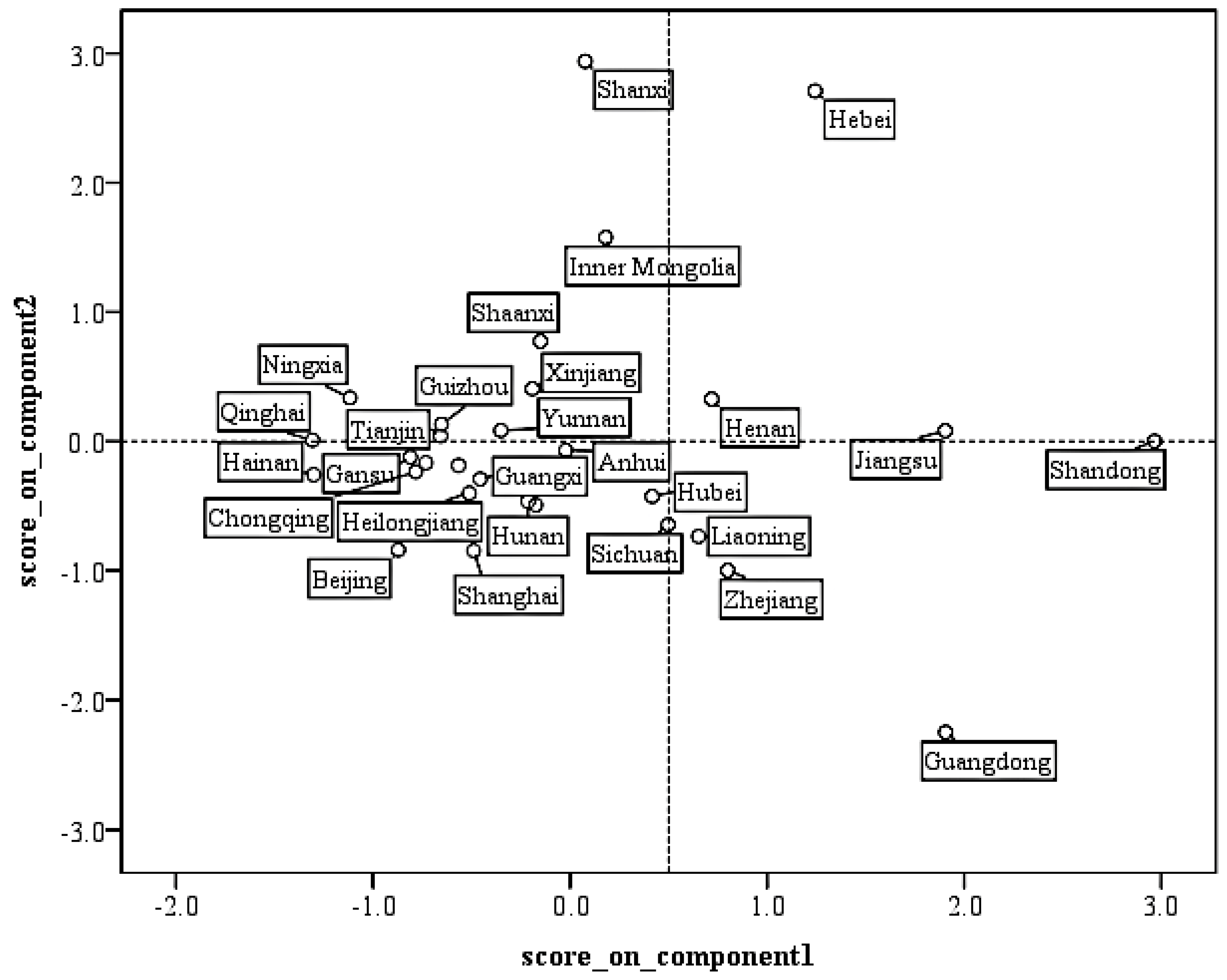
Figure 1 shows the dimensionless scores of 30 provinces on component 1 (the first principal component) and component 2 (the second principal component). The horizontal axis shows the scores on component 1, and the vertical axis shows the scores on component 2. The cumulative contribution of the two components is 71.8%. Shandong, Guangdong and Jiangsu present the highest score on component 1. These three provinces possess high comprehensive productivity, considering that component 1 is the comprehensive polluting factor. Shanxi and Hebei have prominent scores on component 2, which is related to the steel sector; thus, these places achieve high steel productivity. The annual AQI values in 2014 are 120, 68, 107, 97 and 135 in Shandong, Guangdong, Jiangsu, Shanxi and Hebei, respectively. Three of the five provinces, except Shanxi and Guangdong, are amongst the eight provinces with the highest AQI in China. Shanxi has a moderate AQI amongst the mentioned provinces because of its low scores on component 1. Similarly, the low AQI of Guangdong may be due to its low scores on component 2. This finding verifies to some extent the positive relation between AQI and the selected indicators of polluting sectors.

AQI was taken as a dependent variable, and the scores of the original polluting sector data on the four principal components were taken as independent variables. After the standardisation of variables, a linear regression model was established to explore the relationship between annual AQI and polluting capacities quantitatively. The results are shown in

Table 7. Result of linear regression.

Type of Regression	R2	F-Value	p-Value
Linear regression	0.287	2.518	0.067

.

Table 7 presents that the R² of the linear regression model is only 0.287, which means that the model can explain only 28.7% of the information contained in dependent variables. The F-value of the model is 2.518, and the corresponding p-value is significant at the significance level of 0.1, which indicates that there exists a linear correlation between AQI and polluting sectors; however, since the R² is very low, the polluting sectors within an area cannot fully explain AQI.

The coefficients of linear regression are given in

Table 8. Coefficients of linear regression.

Model	Unstandardised Coefficients	T-Value	Significance
(constant)	0	0.000	1.000
Component 1	0.305	1.808	0.083
Component 2	0.348	2.059	0.050
Component 3	0.032	0.192	0.850
Component 4	0.269	1.590	0.124

. The significance of t-test of all independent variables, except component 3, is at an acceptable level. Thus, components 1, 2 and 4 play more important roles in explaining AQI compared with component 3. The non-standardised coefficients of the four common components are all positive, which means that the 13 polluting sectors all act positively in increasing AQI. Component 1 is the comprehensive polluting factor. The component matrix implies that component 1 has high loading values of car ownership, built-up area, diesel consumption and electric power output. Thus, these indicators contribute significantly in explaining AQI. Component 2 is the steel sector factor, and it has the highest unstandardised coefficient; hence, steel sector is the main factor that leads to air pollution. Component 3 has high loading values of fuel oil consumption, caustic soda output and crude oil consumption. This component has a low unstandardised coefficient, and its t-test significance is 0.850. Therefore, the factors that this component represents are non-dominant in increasing AQI. Component 4 has high loading values of plate glass and steel outputs, which also contribute to air pollution.

In conclusion, the results of linear regression indicate that 13 polluting sectors (independent variables) have low explanatory power on AQI (dependent variable), with a poor R² value of 0.287. The spatial correlation of dependent variables should be fully considered for accurate and reliable estimates, and the SAR model is an appropriate method for dealing with this key issue in previous studies.

3.2. Results of the SAR Model

The results of the linear quantitative model show that polluting sectors cannot perfectly explain AQI with a poor R² value of 28.7%. The linear model does not involve the effects of spatial correlations amongst areas. Air pollution can flow easily, leading to trans-boundary pollution. The AQI of a given area is not only affected by the polluting sectors within the area but is also related to the AQI of the adjacent regions. To test the assumption of its spatial correlation, the global Moran’s I test was used to measure the overall correlation of all regions’ AQI. Tibet’s AQI was considered in the global and local Moran’s I tests to provide a whole view of the spatial characteristic of AQI of China. The results are shown in

Table 9. Global Moran’s I test of AQI.

Type of Test	Statistical Value	p-Value
Moran’s I test	0.451	0.001

. The null hypothesis of the global Moran’s I test is that no spatial correlation exists. Table 9 shows the statistical value of the global Moran’s I test in this research is 0.451, and its p-value < 0.01, which indicates that the null hypothesis can be rejected, and a significant spatial correlation exists. Meanwhile, the result of the global Moran’s I test is apparently positive. Therefore, the AQI of a given area is positively affected by those of the adjacent areas.

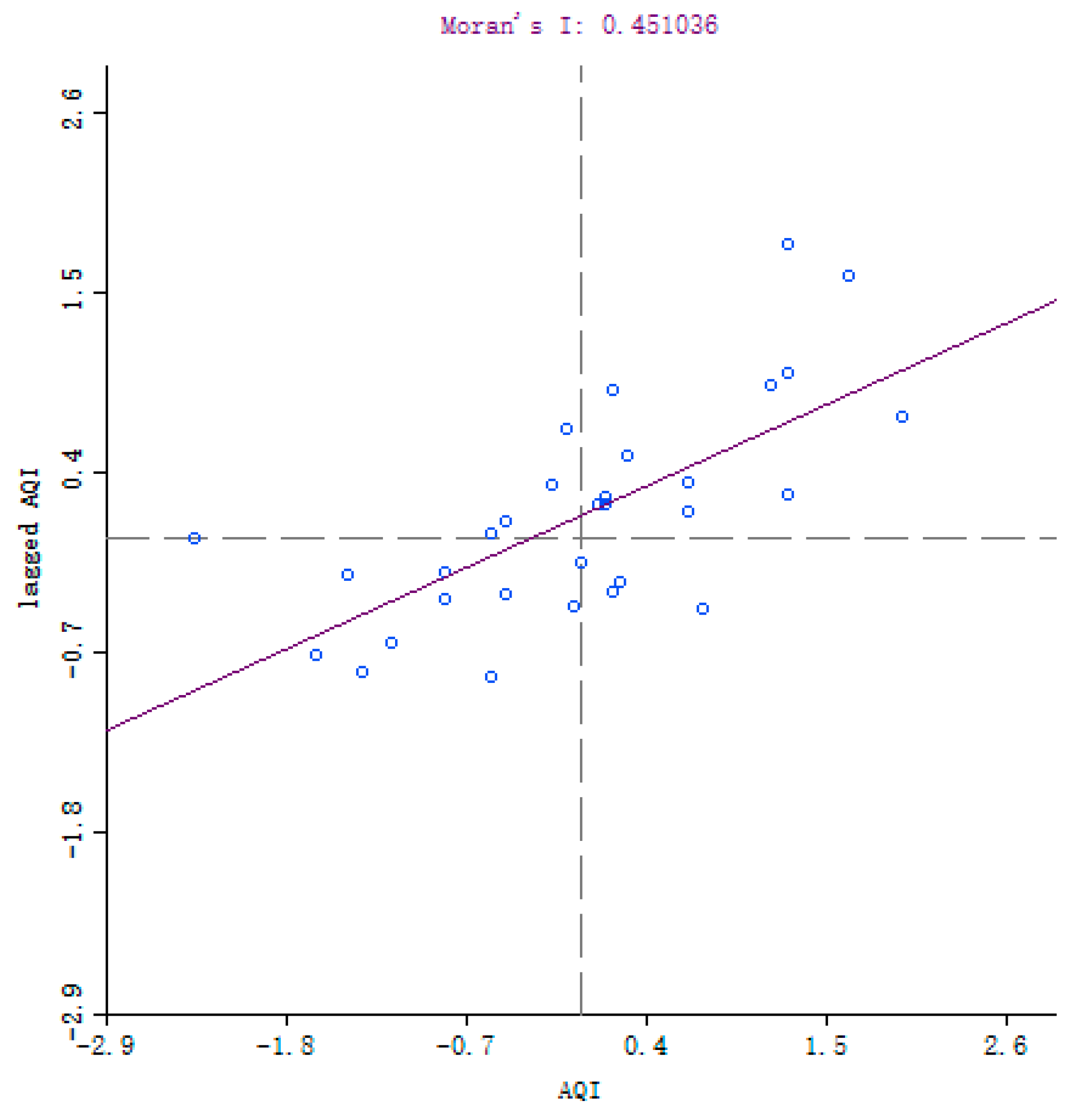
The local Moran’s I test was conducted to further explore the spatial features of local areas. The results can be seen in Figure 2 and Figure 3. The first and third quadrants of the Moran’s index scatterplot indicate a positive spatial correlation, whereas the second and fourth quadrants indicate a negative spatial correlation. Figure 2 and

Table 10. Quadrant distribution of Moran’s index scatterplot.

First Quadrant	Second Quadrant	Third Quadrant	Fourth Quadrant
Tianjin, Beijing, Shandong, Henan, Shanxi, Hebei, Anhui, Chongqing, Ningxia, Gansu, Shanxi, Jiangsu, Hubei	Liaoning, Inner Mongolia, Shanghai, Heilongjiang	Hainan, Tibet, Jiangxi, Zhejiang, Guizhou, Guangdong, Yunnan, Fujian, Guangxi, Sichuan, Qinghai	Jilin, Hunan, Xinjiang

show that most points gather at the first (high–high AQI region aggregation) and the third quadrants (low–low AQI region aggregation), indicating a significantly positive local spatial agglomeration.

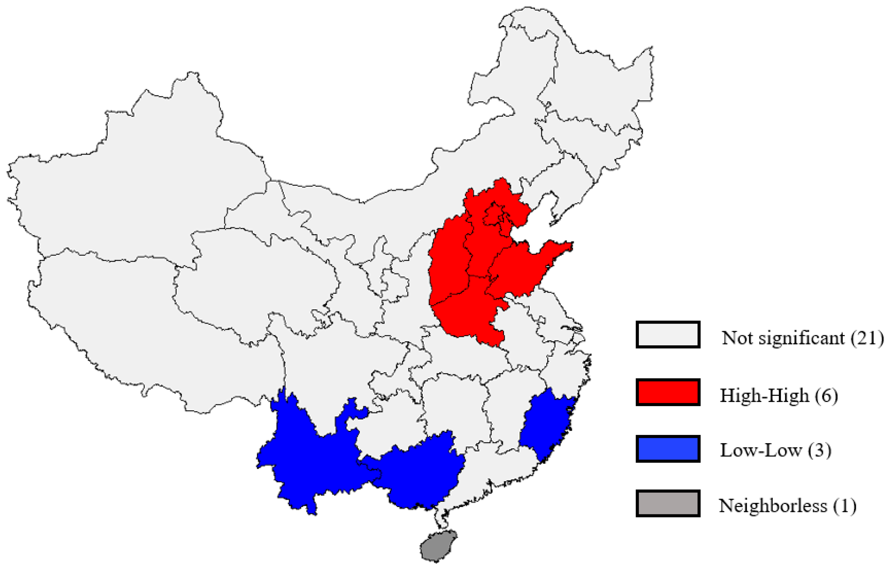
A high value of the local Moran’s I index, namely, positive local spatial auto-correlation, is called spatial aggregation (i.e., high–high or low–low agglomeration), and negative local spatial auto-correlation is called spatial outliers (i.e., high–low or low–high agglomeration). In addition to the Moran’s index scatterplot, the LISA cluster map can also clearly represent these spatial features (Figure 3). The significance test with a significance level of 5% was conducted by using the Monte Carlo method with 999 simulations.

Figure 3 illustrates that many high–high AQI agglomeration regions are situated around the Beijing–Tianjin–Hebei areas and expand to Shandong, Shanxi and Henan provinces. Meanwhile, a great number of low–low AQI agglomeration regions are in south China, including Yunnan, Guangxi and Fujian.

As the AQI data show a significant spatial characteristic, the SAR model is an appropriate method to estimate the relationship amongst AQI, polluting sectors and locations. The SAR model treated standardised AQI as a dependent variable and the standardised scores of the original polluting sector data on the four principal components as independent variables. The result of the SAR model is shown in

Table 11. Result of spatial auto-regression (SAR) model.

Type of Model	R2	$\mathbf{Rho}\left(\mathsf{\rho }\right)$
SAR model	0.705	0.793

and

Table 12. Coefficients of the SAR model.

Model	Unstandardised Coefficients	T-Value	Significance
(constant)	−0.080	−0.815	0.415
Component 1	0.237	2.362	0.018
Component 2	0.137	1.372	0.170
Component 3	−0.110	−1.103	0.270
Component 4	0.144	1.429	0.153

.

The R² of the SAR model is 0.705, which means that this model can explain 70.5% of the dependent variables (Table 11). The spatial correlation coefficient is $\mathsf{\rho }$ = 0.793, consistent with the results of the global Moran’s I test (Table 9), which shows a distinct spatial correlation amongst dependent variables and indicates that a given region’s AQI will rise by approximately 0.793% if the AQI of its ambient regions increase by 1%.

Table 12 shows the coefficients of the auto-regression model. Some conclusions can be drawn by comparing Table 8 and Table 12. In the auto-regression model, the significance of component 1 is 0.018, which is far more significant than that in the regression model (0.083). The unstandardised coefficient of this component is 0.273, which is the highest amongst the values of the four components of the auto-regression model. Hence, component 1 plays an important role in explaining AQI. Component 1 is a comprehensive polluting factor, and its loads of other 13 polluting sectors are all positive. This result means that the other 13 polluting sectors all lead to pollution at varying degrees. The load in Table 6 shows that car ownership, built-up area and diesel consumption are the three most accountable factors in explaining AQI. The result corresponds to the research conducted by Guo et al. [39]. The National Bureau of Statistics presented that the quantity of privately owned cars was 145,981.1 k in 2014. The increase in car use causes an increase in the emission of cars. Guo et al. [39] indicated that car ownership in China experienced an extraordinary growth of 15% in the last decade, and car exhaust has become the key source of air pollutants in urban areas. New energy vehicles may provide a good solution for reducing the influence of cars on the environment [40,41,42].

In the SAR model, the significance of component 2 is 0.170, and its non-standardised coefficient is 0.348, which ranks third amongst the four components. In the linear regression model, the significance of component 2 is 0.050, and its non-standardised coefficient is 0.348, which ranks first amongst the components. Component 2 has the heaviest loads of coke output, coal consumption and steel output, which are related to the steel sector; therefore, component 2 represents the steel sector. The significance of component 2 in explaining AQI is reduced in the auto-regression model. Nevertheless, the coefficient of this component remains important in the two models. Steel sector contributes significantly to air pollution because that steel sector has the features of high energy consumption, emission and pollution, which lead to air pollution and environmental problems, including haze pollution.

In the SAR model, the significance of component 3 is 0.270, and its non-standardised coefficient is −0.110. In the linear regression model, the significance of component 3 is 0.850, and its non-standardised coefficient is 0.032. Component 3 is the least significant component in the two models, and it accounts least for AQI. Component 3 has heavy loads of fuel oil consumption, caustic soda output and crude oil consumption, which means that these three factors are inconsiderably accountable in explaining AQI.

In the SAR model, the significance of component 4 is 0.153, and its non-standardised coefficient is 0.144, which ranks second amongst the four components. In the linear regression model, the significance of component 2 is 0.124, and its non-standardised coefficient is 0.269, which ranks third amongst the components. Component 4 has loads of plate glass and steel outputs. This result reconfirms the significance of steel output in air pollution.

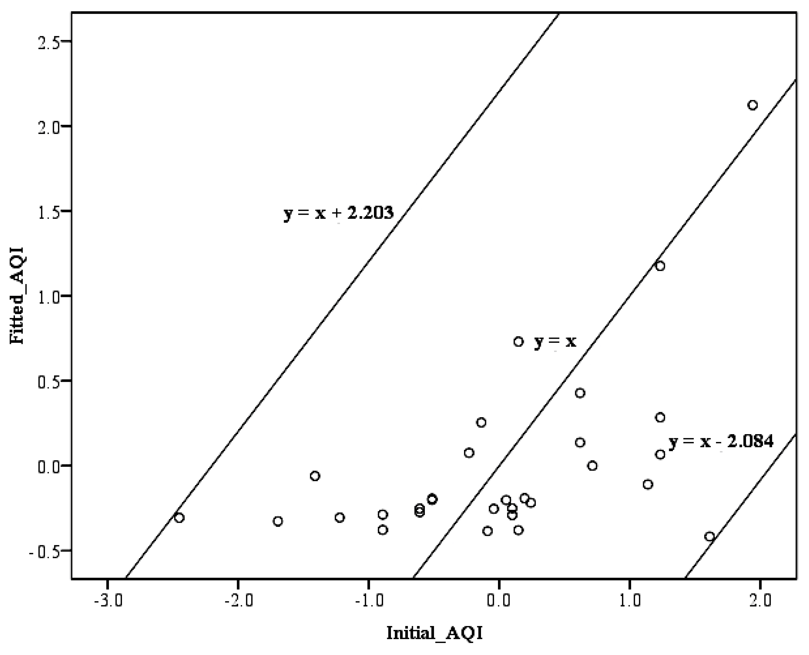
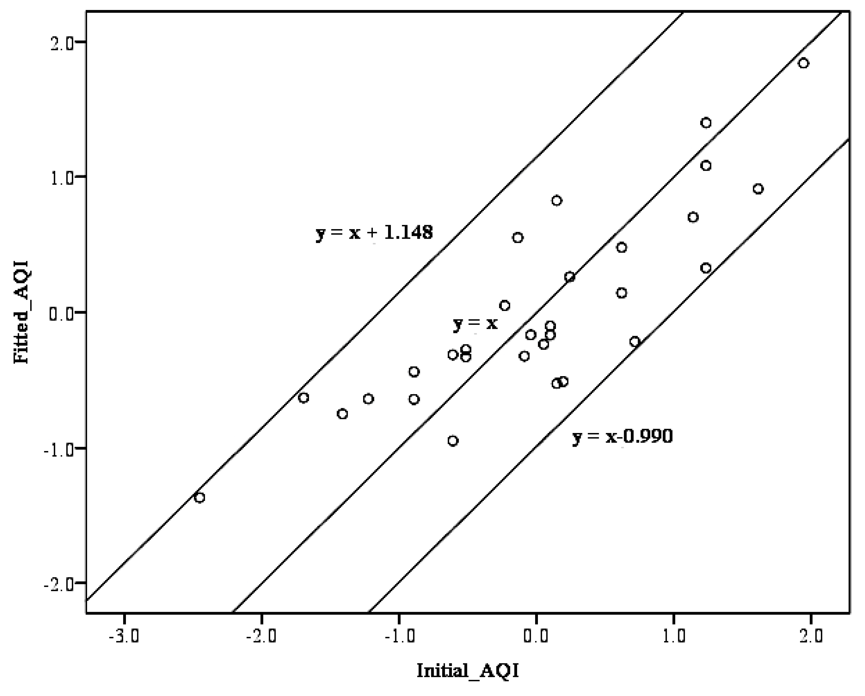
Unlike the linear regression model, the SAR model better explains AQI, with the explanatory power significantly increased from 28.7 to 70.5%. The fitting effect of both models is shown in Figure 4 and Figure 5.

The slopes of straight lines in Figure 4 and Figure 5 are both 1. The intercept of the medium line is 0. The vertical axis represents the standardised fitted value of AQI, and the horizontal axis represents the standardised initial value of AQI. Points close to the medium line indicate a good fitting effect. The ideal effect of fitting is that all points come out on the line, which means that the fitting is perfect. The side lines distinguish the discrete range. Unlike that in Figure 4, the discrete range in Figure 5 is much smaller, and the points are closer to the ideal value and reveal a trend of centralisation. The SAR model, which considers spatial correlation, clearly portrays the AQI of the real condition. Therefore, these two figures further indicate that the SAR model can better explain AQI compared with the linear regression model. The AQI of a given area is not only affected by the polluting sectors within the area but is also related to the AQI of the adjacent areas.

4. Discussion of Stain Map

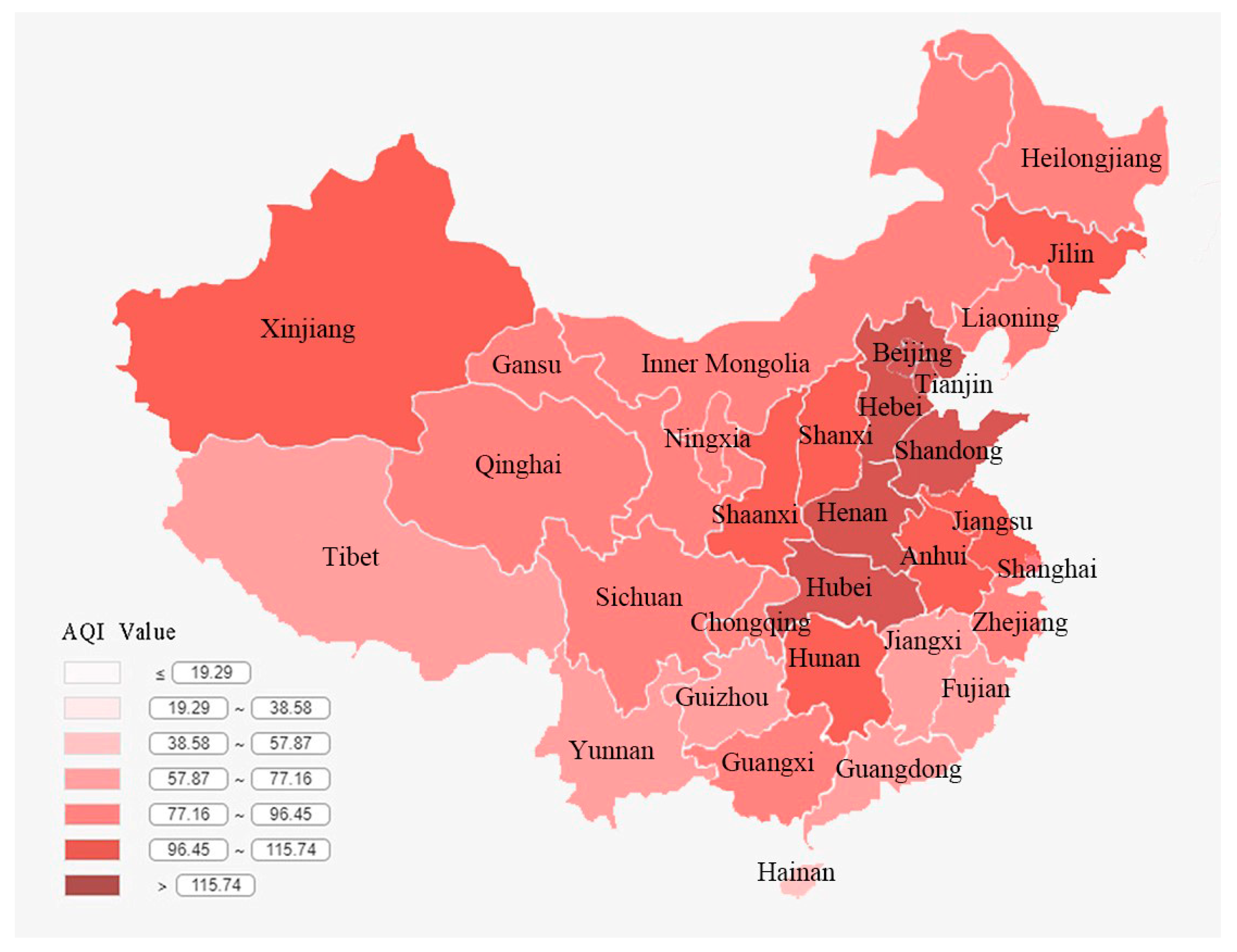
To further reveal the distribution of AQI in 2014 across China and discuss the trans-boundary effect of air pollution in the Beijing–Tianjin–Hebei region, a stain map is shown as Figure 6.

In Figure 6, a darker colour indicates higher AQI, representing worse air quality. The air quality in southern and western China is generally better than that in northern and eastern China. The Tianjin–Beijing–Hebei, Shandong, Hebei and Hubei regions possess the highest AQI and suffer the worst air quality. Figure 3 and Figure 6 show that the clusters of air pollutants mainly occur in the Beijing–Tianjin–Hebei region, Yangtze River Delta and central China, which connects these two economic urban agglomerations. This finding is consistent with the conclusions drawn by Ma and Zhang [8], who argued that industrial restructuring amongst these areas is the main factor affecting the clustering of air pollution. Central China, which connects the Beijing–Tianjin–Hebei region and the Yangtze River Delta, has undertaken industrial transfer, especially high-polluting and high energy-consuming ones, from the two poles of economic urban agglomerations owing to its advantages, such as a favourable location [43]. On the other hand, local government elites strive for high GDP and compete fiercely considering that GDP is an important standard for assessing political achievement [44,45,46]. Disadvantaged and undeveloped areas have no other choice but to develop manufacturing and other high-polluting industries because of the limited number of industries that are clean and can raise GDP greatly in a short time. Liberal policies on the environment are widely used to compete with other local governments for attracting investments, as evident in mid- and western China. However, the developed areas of China, which are adjacent to highly polluted areas, cannot really enjoy all the benefits of their industrial structure optimisation due to the trans-boundary flow of pollutants. When the spillover of pollution overtakes the effect of self-optimisation, the developed areas cannot improve their environment quality.

Figure 1 shows that Beijing and Tianjin are located on the bottom left of the scatter diagram and have low scores on the two components, indicating the low emission of polluting sectors in Beijing and Tianjin. In Beijing, measures aimed at reducing local emission have been used to improve air quality and have been proven to be effective [47,48]. Beijing is amongst the best in the country in the aspect of dismissing polluting sectors and controlling polluting emission [49,50]. However, the air quality in Beijing fails to meet the expectation of citizens. The AQI of Beijing is 128, which is the second highest in China. Similar to Beijing, Tianjin’s emission of polluting sectors is also at a low level, but the AQI of Tianjin is 120, which is the third highest in China. Hence, the high AQI in Beijing and Tianjin cannot be attributed to the mass productivity of polluting sectors but to their unique locations. Figure 6 shows that Beijing is encompassed by Hebei Province, which possesses the highest AQI of 135 in China. In addition, Beijing and Tianjin’s adjacent places, including Shanxi, Shandong and Henan, are areas with high AQI. The high–high AQI aggregation of these regions is illustrated by Figure 3. Hence, the air quality in Beijing and Tianjin is unavoidably affected by their neighbouring regions. The high AQI of Beijing and Tianjin is distinctly caused by the trans-boundary flow of air pollutants from Hebei and nearby provinces.

5. Conclusions and Policy Recommendations

This research investigates the existence of trans-boundary air pollution in China. Linear regression and SAR models were employed to analyse the data of annual concentration of AQI and 13 polluting sectors of 30 provinces and autonomous regions in 2014. Several important findings are derived.

Firstly, the result of the global Moran’s I test is 0.451, which implies that the AQI of China shows distinct characteristics of spatial correlation. The results of the local Moran’s I test show that the regions of high–high AQI agglomeration are located around Beijing–Tianjin–Hebei area and expand to Shandong, Shanxi and Henan; the regions of low–low AQI agglomeration are all in south China, including Yunnan, Guangxi and Fujian.

Secondly, the estimation performance of the SAR model on the relationship between AQI and the standardised scores of the original 13 polluting sector data on the four principal components extracted by non-rotation factor analysis is significantly better than that of the linear regression model. Specifically, the R-squared value is significantly improved from 0.287 to 0.705. The estimation results confirm the existence of trans-boundary air pollution in China. A given region’s AQI will approximately rise by 0.793% if the AQI of its ambient regions increase by 1%.

Thirdly, 13 polluting sectors lead to the rise in AQI in varying degrees. Car ownership, steel output, coke output, coal consumption, built-up area, diesel consumption and electric power output contribute most to air pollution according to AQI, whereas fuel oil consumption, caustic soda output and crude oil consumption are inconsiderably accountable in raising AQI.

Fourthly, according to estimation results of the principle analysis, Beijing and Tianjin have low scores on polluting factor and steel sector factor. The emission of AQI pollutant in Beijing and Tianjin is insignificant, and the high AQI of Beijing and Tianjin is mainly caused by the spatial correlation of air pollution. The trans-boundary flow of air pollution from Hebei and nearby provinces to Beijing and Tianjin is an important contributing factor to poor air quality.

According to the findings of the study, related policy recommendations are proposed as follows:

Firstly, local governments should play the dominant role and actively participate in controlling 13 polluting sectors. According to the regression results, 13 polluting sectors led to the rise in AQI in varying degrees. These 13 polluting sectors should be placed under stringent control; relevant laws aimed at limiting polluting sectors should be enacted and reinforced; and the emission of polluting sectors during production should be closely monitored. The steel sector is highly polluting and has been the main source of air pollution, according to the results of regression models. Thus, the government should adjust fiscal policy to encourage the steel sector to reduce emissions, upgrade its technology and equipment, and encourage and support green production.

Secondly, in addition to polluting sectors, the trans-boundary flow of pollutants significantly contributes to the high value of AQI. According to SAR model, a given region’s AQI will rise by 0.793% if the AQI of its ambient region increases by 1%, and so regional cooperation should be strengthened to govern air pollution. Breaking the governance boundary and working jointly to design and practice pollution control are important. Policy recommendations are made for the Beijing–Tianjin–Hebei region, which has a high AQI agglomeration according to the local Moran’s I test. The establishment of a joint enforcement policing system in the three locations will deepen the coordination and linkage mechanism. A pollution detection network system should be established to realise all-day and all-domain monitoring of air pollution to accurately monitor and control the emission sources of important pollutants. In addition, the Beijing–Tianjin–Hebei region can use weather forecast data to proactively mitigate pollution emission. For example, under extreme circumstances such as heavy air pollution or important events, the high-polluting factories located in the upwind direction of Beijing should reduce or stop production in advance to avoid the formation of air pollution, particularly for those factories with outdated exhaust gas treatment technology.

Thirdly, Figure 3 and Figure 6 show that the clusters of air pollutants mainly occur in the Beijing–Tianjin–Hebei region, Yangtze River Delta and central China, which connects these two economic urban agglomerations. The high-polluting and high-energy-consuming sectors are mainly located among the two poles of economic urban agglomerations. China should take advantage of developed railway transportation network, inward industrial development in the west, which can make good use of a landlocked resource, drive the growth of the western economy, and relieve air pollution in the east.

Fourthly, some indicators relevant to inhabitants, such as car ownership and electric power outputs, lead to air pollution. Therefore, inhabitants are indispensable factors in pollution control. The government should encourage the inhabitants to prioritise environment-friendly and low-carbon transportation means, such as bicycles, buses and electric automobiles. Cars, especially those that do not meet exhaust emission standards, should be strictly prohibited from roads. The government should also improve the consciousness of inhabitants in protecting the environment and instil the concept of a low-carbon lifestyle in their minds and advocate for low-carbon habits, such as turning off lights when leaving a room [51].