Article

Equitable Allocation of Blue and Green Water Footprints Based on Land-Use Types: A Case Study of the Yangtze River Economic Belt

1
State Key Laboratory of Hydrology of Water Resources and Hydraulic Engineering, Hohai University, Nanjing 210098, China
2
Institute of Management Science, Hohai University, Nanjing 210098, China
3
Hohai University Coastal Development and Protection Collaborative Innovation Center, Nanjing 210098, China
4
College of Economics and Management, Fuzhou University, Fuzhou, Fujian 350116, China
5
Odette School of Business, University of Windsor, Windsor, ON N9B 3P4, Canada
*
Author to whom correspondence should be addressed.
Sustainability 2018, 10(10), 3556; https://doi.org/10.3390/su10103556
Submission received: 24 August 2018 / Revised: 2 October 2018 / Accepted: 2 October 2018 / Published: 4 October 2018
(This article belongs to the Special Issue Conflict Analysis and Sustainable Management of Water Resources)

Abstract

:
This paper develops a lexicographic optimization model to allocate agricultural and non-agricultural water footprints by using the land area as the influencing factor. An index known as the water-footprint-land density (WFLD) index is then put forward to assess the impact and equity of the resulting allocation scheme. Subsequently, the proposed model is applied to a case study allocating water resources for the 11 provinces and municipalities in the Yangtze River Economic Belt (YREB). The objective is to achieve equitable spatial allocation of water resources from a water footprint perspective. Based on the statistical data in 2013, this approach starts with a proper accounting for water footprints in the 11 YREB provinces. We then determined an optimal allocation of water footprints by using the proposed lexicographic optimization approach from a land area angle. Lastly, we analyzed how different types of land uses contribute to allocation equity and we discuss policy changes to implement the optimal allocation schemes in the YREB. Analytical results show that: (1) the optimized agricultural and non-agricultural water footprints decrease from the current levels for each province across the YREB, but this decrease shows a heterogeneous pattern; (2) the WFLD of 11 YREB provinces all decline after optimization with the largest decline in Shanghai and the smallest decline in Sichuan; and (3) the impact of agricultural land on the allocation of agricultural water footprints is mainly reflected in the land use structure of three land types including arable land, forest land, and grassland. The different land use structures in the upstream, midstream, and downstream regions lead to the spatial heterogeneity of the optimized agricultural water footprints in the three YREB segments; (4) In addition to the non-agricultural land area, different regional industrial structures are the main reason for the spatial heterogeneity of the optimized non-agricultural water footprints. Our water-footprint-based optimal water resources allocation scheme helps alleviate the water resources shortage pressure and achieve coordinated and balanced development in the YREB.

1. Introduction

Water is one of the most precious natural resources on which human beings rely. Global climate change and the ever-increasing population lead to numerous conflicts over water rights due to the scarcity of water resources. Water shortage has arisen as a critical bottleneck for economic development and prosperity around the globe. The United Nations World Water Development Report of 2017 [1] shows that two-thirds of the world population lives in drylands with varying degrees of a water shortage. Ecological problems caused by a water shortage become increasingly severe, which make the ecological environment more and more fragile and vulnerable. Recent rapid economic and societal development results in a higher consumption of water resources per capita and exacerbates water resource shortages, which makes the contradiction between human and water increasingly prominent. As such, it has become an urgent and widespread challenge to optimally allocate scarce water resources in many parts of the world.
Jerson and Rafael [2] propose a water resource allocation model for different water users where the carrying capacity of water resources is unable to meet the demand of the economy. Eleftheriadou and Mylopoulos [3] employ game theory to examine the conflict arising from transboundary water resources management. Liehr et al. [4] address water resources management problems arising from social and natural conflicts from an interdisciplinary perspective. These traditional methods mainly focus on allocating the water quantity without accounting for structural adjustments of water supply and demand. To this end, a new indicator known as the water footprint is proposed to gauge the structure of the water supply and demand. Water footprint refers to the amount of water resources required for all the products and services consumed by a country, a region, or a person within a certain period of time. Since Hoekstra [5] first proposed the concept of the water footprint in 2003, extensive research has been carried out to investigate the water footprint and its related problems. Kampman et al. [6], Van Oel et al. [7], and Chapagain and Orr [8], respectively, compare the water footprint of India, the Netherlands, and the UK with their actual available water resources and identify key areas of water shortages. Ma et al. [9] study the water footprints in Beijing and find that the water footprint per capita is nearly 10 times higher than the volume of available water resources. Casolani et al. [10] investigate water and carbon footprints in Italian durum wheat cultivation and find a high ratio of water footprints to the total agricultural land area. Since water footprints account for water consumption in the process of human production and living activities, it must be expanded on a spatial scale to enable proper accounting and management of water footprints [11]. Land area, as an index to describe spatial distributions, has been used by many scholars as a key indicator for equitably allocating water resources. Salmoral et al. [12] study the impact of different agricultural land use types on water footprints with an aim to comprehensively manage land and water resources. Sun et al. [13] identify land as a key influencing factor of the regional flood disaster resilience in the Lake Chao Basin. Dong et al. [14] examine the fairness of water uses in China from 1997 to 2011 by, respectively, selecting population, GDP (Gross Domestic Product), the arable land area, and water resources as the evaluation indicator. Their result shows that the arable land area and water resources are two important factors affecting the fairness of water uses in China.
Due to water resources’ quasi-public goods nature, the United Nations Economic and Social Commission for Asia and the Pacific (UNESCAP) notes that the core principles of water resources management are equity, efficiency, and sustainability [15]. Therefore, water resource allocation should take these three principles as the basis. Mimi and Sawalhi [16] establish a fair allocation index system for allocating water resources in the Jordan River Basin. Current research on the fairness of water resource allocation mainly focuses on evaluating the fairness of water uses and limited research considers quantitative approaches to fair allocation of water resources. Along this line, the lexicographic minimax algorithm [17] has a wide range of applications thanks to its advantage of being fair to different users and being simple and fast to calculate. Ogryczak et al. [18] proposed a set of well-stated principles of fair resource allocation as “monotonicity, impartiality, and equitability.” Different functions can be used to characterize this set of fairness principles [19]. For instance, Yager’s [20] ordered that the weighted averaging (OWA) aggregation operator is proved to satisfy Ogryczak’s fairness principles [18]. When the subjects of configuration are finite, the OWA aggregation approximates the ranking order generated by the lexicographic ranking approach [19].
In multi-objective decision making, the lexicographic minimax algorithm finds a solution by repeatedly solving problems with a minimax objective function, which determines Pareto optimal solutions while ensuring fairness. Luss and Smith [21] employ successive lexicographic minimax algorithms to allocate raw materials in industrial production. Wang [22] improves the algorithms proposed by Luss [17] and constructs a series of fair allocation models for basin water resources. Generally, for resource allocation with a small number of participants, the algorithms in References [17,21] can be expeditiously executed. For allocation problems with a large number of users, the programming algorithms proposed in Reference [22] prove to be convenient tools. Buzna et al. [23] propose an approximate lexicographic minimax algorithm for solving discrete facility location problems.
In 2016, the Chinese Ministry of Water Resources and Ministry of Land and Resources issued a joint “Pilot Program for Ascertaining Water Property Rights” to delimit the scope of waters, shorelines, and other water ecological space and to determine the ownership of water ecological space. A recent research report on China’s water resource strategies identifies eight critical changes such as “from neglecting to ensuring water uses for the ecological environment when water resources are allocated” to achieve sustainable development [24]. These documents provide strategic guidelines for water resource management in regions with highly intensive human activity. In allocating water resources in these regions, a holistic approach should be taken by examining the life cycle of water resources, looking beyond the traditional amount-based allocation model, and optimizing the structural supply and demand. To this end, the water-footprint-based allocation scheme arises as a natural choice to account for the actual usage of regional water resources. Generally speaking, the imbalance between supply and demand of water resources in an area creates conflict between the human and the environment and results in obstacles for regional sustainable development. As such, it is crucial to allocate water resources among competing users in a fair, efficient, and sustainable manner. Given the significance and necessity of sustainable management of water resources, this research introduces a water footprint perspective to optimize the structural supply and demand of water resources. The resulting scheme is able to rebalance the uses of water resources among competing users in the area. To equitably allocate water resources, this paper adopts the lexicographic minimax algorithm. By using land area as the influencing factor, a lexicographic optimization model is established for allocating blue and green water footprints.
Next, we establish a water footprint accounting model. We then propose a model to measure the WFLD. By using the Yangtze River Economic Belt (YREB) as a case study, we apply the previously mentioned method to perform a cross-scale analysis and categorization of land uses for lexicographic allocation of blue and green water footprints in the YREB. The purpose is to furnish a new angle to examine the water resources conflict among different stakeholders in the area. By properly characterizing water demand patterns and analyzing their relationship with different types of land uses, the proposed approach aims to achieve a balance between supply and demand of water resources in the area. Analytical results shed significant insight into the structural adjustment of land uses in different industries as well as into the furnish strategies to improve water use efficiency and promote healthy and sustainable development in the YREB.

2. Materials and Methods

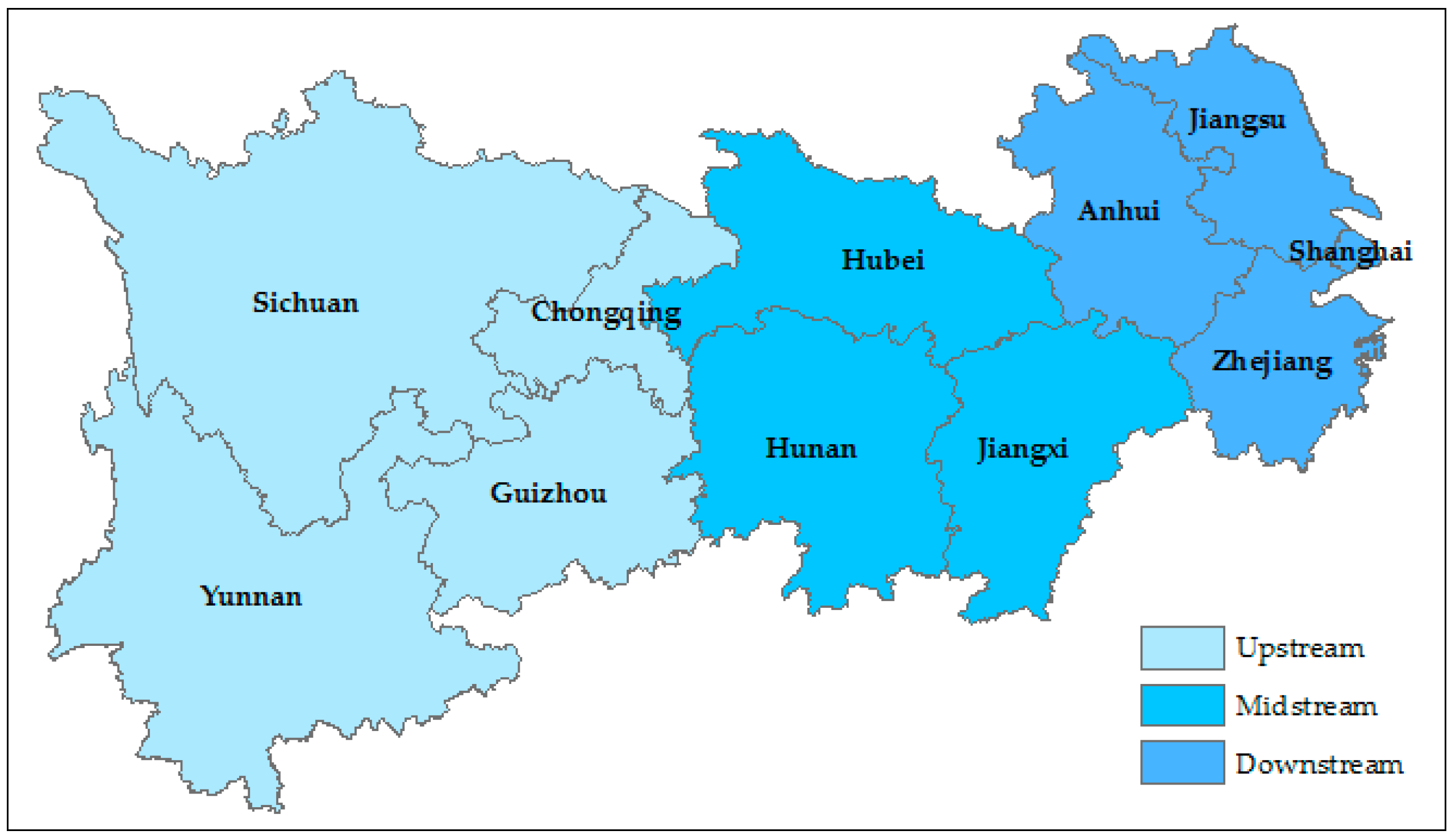
2.1. Region under Investigation

In 2014, China identified leading regional economic development strategies as the One Belt and One Road initiative, Beijing-Tianjin-Hebei coordinated development, and the YREB. Among these strategies, the YREB plays a critical role in the success of the One Belt and the One Road initiative since it is the powerhouse and commodity production base of the Chinese economy. The YREB refers to the Yangtze River and its tributaries extending from the east (Shanghai) to the west (Yunnan) and consisting of nine provinces and two provincial-level municipalities in the Yangtze River Basin except for Qinghai and Tibet. It covers an area of 2.05 million square kilometers and accounts for more than 40% of the nation’s population and GDP. Figure 1 shows the map of the YREB.
As shown in Figure 1, based on the location, the YREB can be divided into three regions including the upstream, the midstream, and the downstream regions. The upstream region includes three provinces (Sichuan, Yunnan, and Guizhou) and one provincial-level municipality (Chongqing). The midstream region comprises three provinces (Hubei, Hunan, and Jiangxi). The downstream region constitutes three provinces (Anhui, Jiangsu, and Zhejiang) and one provincial-level municipality (Shanghai). These three regions are highlighted in different colors in Figure 1. For the sake of conciseness, from this point on, we refer to these 11 provincial-level jurisdictions as provinces without distinguishing a province from a provincial-level municipality. The YREB possesses unique advantages and great potentials for further development as a high-density economic corridor. The “Guidelines of the YREB Development Plan” stresses that Yangtze River economic development must adhere to the overall strategy of “ecology first, green development, coordinated environmental protection, and no further large-scale development projects.”

2.2. Data Collection

This paper selects the previously mentioned 11 provinces in the YREB as the area of investigation. The economic and water resources data are collected from the “China Statistical Yearbook (2014),” the ”Statistical Yearbook (2014)” of the 11 provinces, the “China Environmental Statistical Yearbook (2014),” the “China Water Resources Bulletin (2013),” and the “Yangtze River Basin and Southwest River Water Resources Bulletin (2013).” The meteorological data are drawn from the China Meteorological Data Network (http://data.cma.cn/), and the crop coefficient data are gathered from the Food and Agriculture Organization (FAO) database (http://www.fao.org). Cultivated crops in this area mainly consist of paddy rice, wheat, corn, sorghum, beans, potato, peanut, rapeseed, tobacco, vegetables, fruits among others, and livestock products including beef, lamb, pork, chicken, milk, eggs, and more. Table 1 below shows the basic data on land area, population, GDP, and the available and consumption of water resources in the 11 YREB provinces. It should be stressed that a significant portion of the available water resources given in Table 1 cannot be utilized for human production and living activities due to a lack of proper infrastructures especially in the mountainous areas in the upstream and midstream regions. More detailed data for the water footprint and the land use type are given in Appendix B and Appendix C, respectively.

2.3. Models

It is a challenge to conduct a cross-scale analysis and categorization of land uses for the lexicographic allocation of basin water footprints. Surface and groundwater resources are the main water supply for human production and living activities and they are significantly affected by different types of land uses. Theoretically, water footprints consist of blue, green, and grey components. However, given the current water resources management practice in China, the allocation of grey water resources remains at the very early exploratory stage and has a long way to go before its possible implementation. Even though grey water footprints have been considered for the Haihe River basin [27], limited data on grey water are published in the YREB to allow for a reliable estimate of grey water footprints. This lack of data and practice has led researchers to omit grey water footprints and focus on blue and green water footprints in their studies on water resources management in China [28,29,30]. Therefore, this paper focuses on blue and green water footprints and does not consider the grey water footprint. Without causing confusion, we shall refer to blue and green water footprints simply as water footprints going forward.
It is assumed that there are n entities in the watershed that participate in fair allocation of water resources. It is further assumed that the levels of agricultural cultivation, urban construction, and ecological development are all reasonable and there does not exist over-exploitation of land beyond its carrying capacity or that land development has not caused permanent damage that affects its reutilization. First, a water footprint accounting model is constructed based on two broad types of land uses (agricultural and non-agricultural) to characterize the provincial-level water demand structure in the YREB as agricultural and non-agricultural water footprints. Agricultural water footprints in Model (1) consist of crop evapotranspiration and water consumption of animals during their life spans (including the virtual water content in the feed). Non-agricultural water footprints in Model (2) include industrial production water uses, virtual water content in import and export trade, domestic water consumption, and urban greening water uses. After water footprints are properly accounted, we then propose a lexicographic minimax model (Equation (3)) to minimize the maximum shortage of agricultural and non-agricultural water footprints in each province, according to the corresponding land area. The shortage indicator is expressed as a function of the original water footprints and the target optimal water footprints, f t ( x i ) = W F t i x t i W F t i . Second, to study the relationship between human production and living activities and water and land resources, a WFLD formula is established to describe the carrying capacity of land for human water demand.

2.3.1. A Water Footprint Accounting Model

Next, we calculate the original water footprints (WFi) of the 11 provinces and municipalities in the YREB based on the 2013 statistical data. WFi is decomposed into agricultural ( W F a i ) and non-agricultural water footprints ( W F n i ), where the latter includes industrial, domestic, and urban greening water footprints. First, the CROPWAT model and the production tree method [31] are used to account for agricultural water footprints, which is shown below.
W F a i = j 10 K i j d E T i j ( d ) S i j G i j + k M i k b i r t h s l a u g h t e r { w a t e r i k d + w a t e r i k , s e r v e + w a t e r i k a + h S W D ( h ) × C i k ( h ) } d t w e i g h t i k a  
In Model (1), the subscript i, j, and k refer to province i, crop j, and animal k, respectively. Kij is the average crop coefficient during the cultivation period and we use the FAO recommended values in our calculation due to a lack of region-specific statistical data in the area of investigation. ETij (mm/day) is the daily evapotranspiration of planted crop j. The factor 10 converts mm into m3/km2 and the inner summation accounts for the total evapotranspiration from day 1 to the final day of the cultivation period [32]. Gij (ton/km2) is the unit output of crop j. Sij (ton/year) is the total annual output of crop j. Mik (ton/year) is the annual output of animal k in province i. waterikd (m3/day) indicates the daily amount of water consumed by animal k and waterik,serve (m3/d) represents the total volume of water used to clean the farmyard and the animal as well as other services necessary to maintain the environment during the entire life span of animal k. The amount of water consumed by an animal from the fodder during its life span consists of two parts. The first part is waterika (m3/d), which stands for the actual water required for preparing the feed. The second part is the virtual water incorporated into various fodder components. SWD(h) (m3/ton) denotes water demand of feed crop h and Cik(h) (ton/day) signifies the quantity of feed crop h consumed by animal k. weightika (ton) is the live weight of animal k at the end of its life span. Second, the non-agricultural water footprint W F n i is determined by the equation below.
W F n i = Q i M I P i I O + V W i I V W i O + g U i g P i g + A i η i E P i  
In this model, QiMI (m3/RMB) is the water consumption per ten thousand yuan of Renminbi (the Chinese currency) of industrial product and PiIO (RMB/year) is the gross industrial product in 10,000 RMB. VWiI (m3/year) is the virtual water amount due to inter-provincial import trade and VWiO (m3/year) is the virtual water amount owing to inter-provincial export trade. Uig (m3/person) is the per capita water quota, Pig (person/year) is the annual population, Ai (km2) is the urban area, ηi is the urban greening coverage excluding water surface, and EPi (m3/km2·year) is the annual evapotranspiration of plants per unit area.
This paper assumes that the target of the water footprint optimization for each province in the area is x i , 0 x i W F i ,   i = 1 , 2 , , n , where WFi is the upper bound of the water footprint in province i given by the original water footprints. Loosely speaking, xi and WFi can be treated as the supply and demand of water resources in province i, respectively. Qi (m3) is the available water quantity in province i. Consistent with the accounting of water footprints from agricultural and non-agricultural perspectives in Models (1) and (2), the allocation is also carried out along these two lines: xi = xai + xni and WFi = WFai + WFni. Then f t ( x i ) = W F t i x t i W F t i signifies the scarcity indicator for agricultural (t = a) and non-agricultural water (t = n) footprints: f t ( x i ) < 0 indicates that the water supply of province i exceeds its water demand, f t ( x i ) > 0 means that the water supply is below the demand in province i, and f t ( x i ) = 0 corresponds to the balanced scenario in province i. To address the optimal and equitable allocation of provincial water footprints with finite subjects using land area as the influencing factor, a lexicographic minimax model is introduced below.
L e x min x [ α t i f t ( x i ) ] = L e x min x [ α t i W F t i x t i W F t i ] s . t . { α t i = { L A t i i L A t i | 0 < α t i < 1 } , t { a , n } 0 t { a , n } i N ( α t i x t i ) i N Q i Q _ t i x t i Q ¯ t i i N
In the objective function, t = a, n indexes the agricultural and non-agricultural water footprint, respectively. L A a i ( L A n i ) is the agricultural (non-agricultural) land area in province i in km2. α a i ( α n i ) is the influencing factor of agricultural (non-agricultural) land denoted by the percentage of province i’s agricultural (non-agricultural) land area in the total agricultural (non-agricultural) land area in the whole YREB.
In Model (3), the objective function is to iteratively minimize the maximum shortage of land-area-adjusted agricultural (non-agricultural) water footprints in the n provinces in a lexicographic order. The first equality constraint defines the influencing factor ( α t i , t = a , n ) as the ratio of the agricultural and non-agricultural land area in each province (LAai) relative to the corresponding total in the YREB, respectively. The second inequality constraint ensures that the total allocated water footprint adjusted by agricultural and non-agricultural land areas in all the provinces is within its available water resources and the last inequality constraint specifies the upper ( Q ¯ t i ) and lower bounds ( Q _ t i ) for the allocated agricultural and non-agricultural water footprints in each province. Given the actual water resources distribution in the YREB, t { a , n } i N Q _ t i i N Q i is assumed to guarantee the existence of an optimal solution (i.e., the basic needs of all provinces can be satisfied by properly allocating water resources in the whole area). In addition, there exists at least one province i such that its original water footprint WFi = WFai + WFni satisfies W F a i + W F n i Q i (i.e., at least one province is in shortage of water resources from a water footprint aspect). This ensures that the optimal solution L e x min > 0.
To solve Model (3), the lexicographic minimax algorithm is employed to ensure that the allocation conforms to the principle of fairness [22]. The land-area-based weight factors α a i and α n i furnish one angle to achieve fair, efficient, and sustainable water footprint allocation in the YREB given available water resources [33]. For detailed descriptions of the solution procedure, readers are referred to Appendix A.

2.3.2. A Water-Footprint-Land Density Formula

Water-Footprint-Land Density (WFLD) is an indicator to measure the density of water footprints per unit land area, which is defined by the equation below.
W F L D i = W F i L A i  
where WFi and LAi are, respectively, the total water footprint and the total land area in province i. The smaller the WFLD, the less the water footprint is consumed per unit land area and the stronger the spatial carrying capacity of water resources and vice versa.

3. Modeling Scenarios

To alleviate the pressure of water uses in the 11 YREB provinces and enhance water use efficiency, this paper employs the lexicographic minimax algorithm to equitably allocate water resources with the agricultural and non-agricultural land area as the influencing factor. This algorithm is characterized by an iterative process. The optimal water footprints are obtained iteratively by changing the iterative control parameter a and solving a series of linear programs. The iterative process achieves the optimal value until the absolute deviation | a i x a i | is minimized. Table 2 and Table 3 show several iterative results with intermediate parameter values of the lexicographic minimax solution process from the agricultural and non-agricultural water footprint perspective, respectively.
The allocation of agricultural and non-agricultural water footprints follows the same lexicographic optimization process given in Model (3). Taking the agricultural water footprint optimization as an example, the algorithm starts with any initial estimated aggregate agricultural water footprint value of a and solves the lexicographic minimax Model (3) for optimal x a i iteratively. The difference a i x a i is then determined for this iteration. The next iteration plugs in a new trial value of a to minimize the absolute deviation | a i x a i | . Table 2 illustrates the iterative process of obtaining the optimal solution and shows the values of several parameters where T = i I W F a i a stands for the difference between the current aggregate agricultural water footprint and the estimated value at each iteration. R = i I ( W F a i / α a i ) gives the current aggregate agricultural-land-area adjusted water footprints, k = T / R is a dimensionless ratio between the aforesaid two water footprints, and a v g = a / i N L A i gives the average agricultural water footprint per unit land area across the YREB. Based on the iteration results in Table 2, one can see that | a i x a i | decreases when a increases from 400 billion m3 to 480 billion m3 and the absolute deviation increases in a when it goes beyond 490 billion m3. By the iterative process, one can find that a = i x i at a1 = 485.63 and the corresponding x i gives us the optimal solution for this lexicographic minimax problem. Similarly, Table 3 presents the same optimization process for the non-agricultural water footprint. At a2 = 83.73, the optimal solution is attained for the non-agricultural water footprint lexicographic configuration. The detailed lexicographic optimization solution process is shown in Appendix A.

4. Results

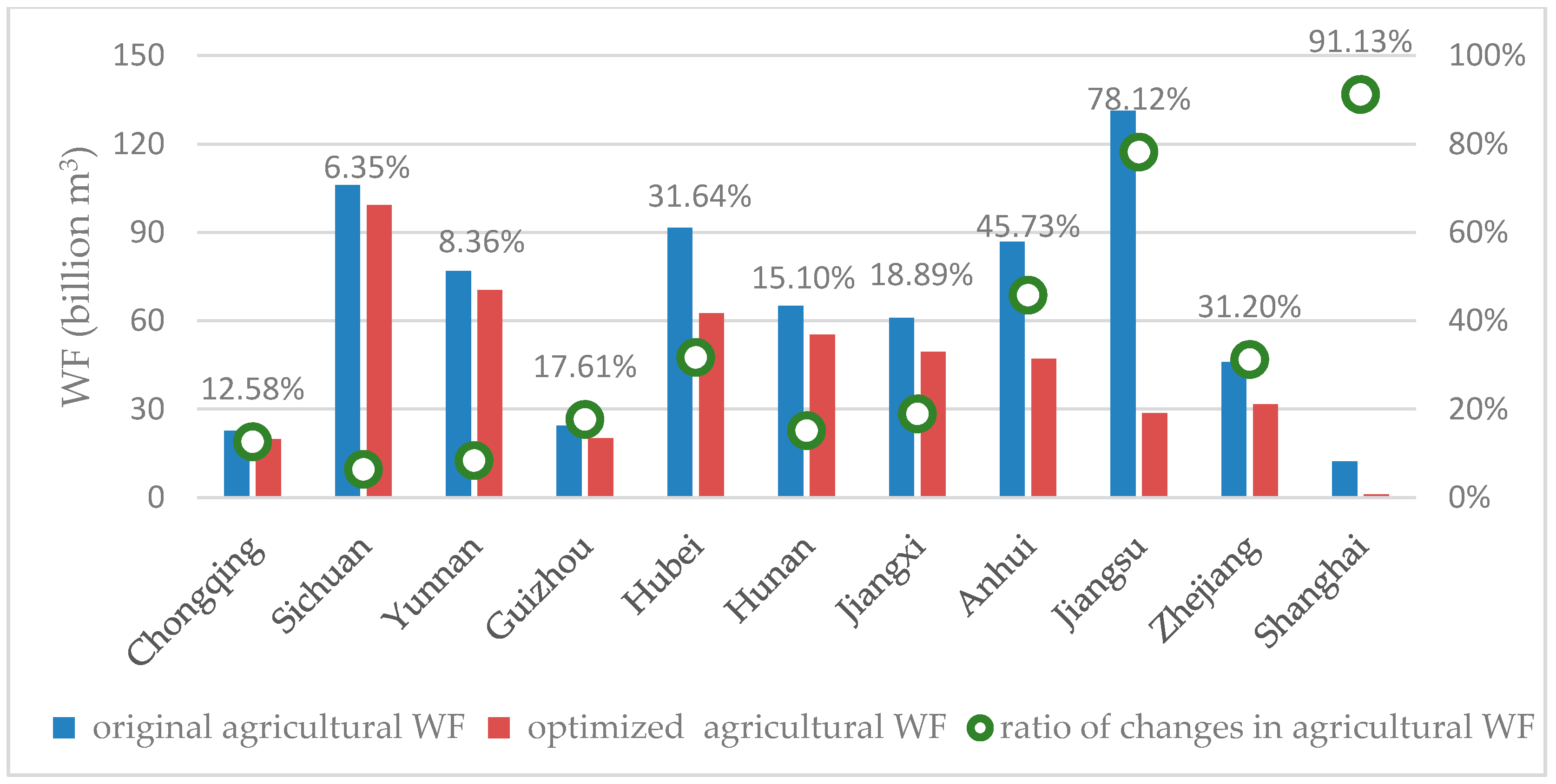
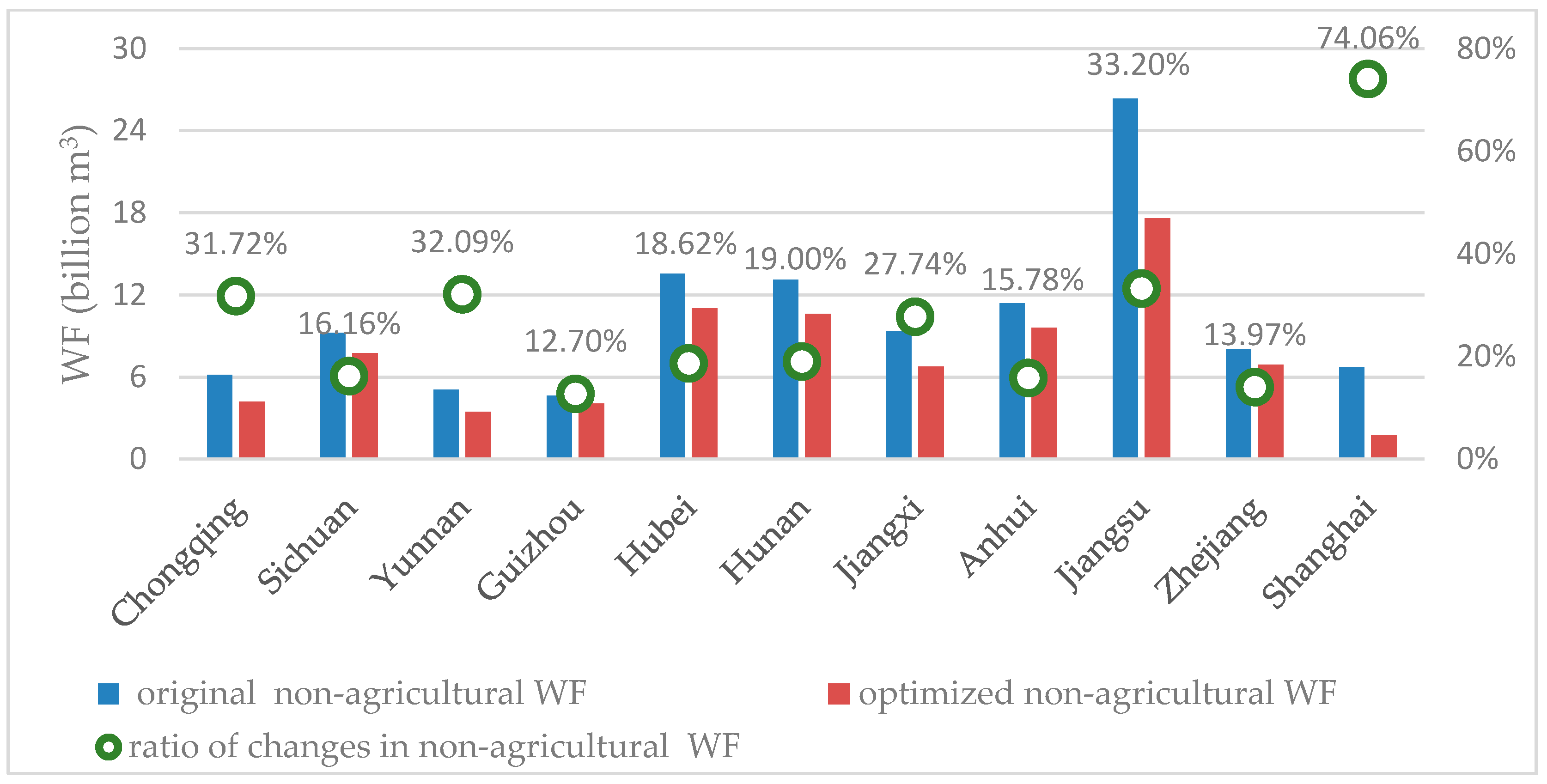
4.1. The Allocation Scheme of Agricultural and Non-Agricultural Water Footprints

Based on the optimal solution at a1 = 485.63 and a2 = 83.73 in Table 2 and Table 3, one can obtain the corresponding optimal agricultural and non-agricultural water footprints for the 11 provinces as shown in the fifth and sixth columns in Table 4 from which one obtains the corresponding total water footprints in the last column.
Water footprints account for water demand for agricultural and non-agricultural (industrial, domestic, urban greening) uses. The original water footprints for the 11 provinces are furnished in the second column of Table 4 and are calculated by using Models (1) and (2) based on the raw data in Table A1 and Table A2 in Appendix B where the last row in Table A1 and Table A2 displays the computed agricultural and non-agricultural water footprints, respectively. Therefore, the second column in Table 4 is obtained by adding up the original agricultural and non-agricultural water footprints in the third and fourth columns.
From Table 4 and Figure 2, we can see that the agricultural water footprint in the YREB under the optimal lexicographic allocation of basin water footprints (LABW) shows a significant decrease from the original level with a total reduction of 32.93%. The original agricultural water footprints account for 86.43% of the original total in the YREB (Table 4). A further analysis of the reduction in agricultural water footprints reveals that, first, the ratio of agricultural water footprints in the upstream, midstream, and downstream regions is changed from 10:9.5:12 to 10:8:5.2 after optimization. Given the agricultural land area data in Appendix C, one can verify that the land area ratio of the three segments is given as 10:4.9:3.1. It is apparent that the LABW optimal allocation scheme for agricultural water resources is more compatible with the spatial distribution of agricultural land in the YREB. Second, reductions of agricultural water footprints show a strong heterogeneous trend in the three segments of the YREB, which is displayed in Figure 2. Overall, agricultural water footprints for the whole YREB decline by 32.43% (Table 4) from the original value to optimized values, but the average percentage declines in the upstream, midstream, and downstream regions vary significantly at 11.22%, 21.88%, and 61.55%, respectively. The decline shows a clear trend that the more economically developed provinces in the downstream region are required to take more responsibility in reducing their agricultural water uses than those upstream traditional agricultural provinces. Lastly, as shown in the three dashed horizontal lines in Figure 2, the percentage declines in agricultural water footprints of the 11 YREB provinces can be divided into three categories. It is not a coincidence that the decline rates of Shanghai and Jiangsu are the highest at 91.13% and 78.12%, respectively, since they are the two main industrial powerhouses in China and have more means to exploiting alternative freshwater sources (e.g., sea water desalination) and absorbing the significant drop without jeopardizing the livelihood of local farmers. The provinces with mid-range declines are Hubei, Anhui, and Zhejiang in which the declines equaled 31.64%, 45.73%, and 31.20%, respectively. The percentage reductions are much more modest in the traditional agricultural provinces in the upstream region as well as Hunan and Jiangxi in the midstream region with an average decrease of 13.15%. Overall, the decline in optimized agricultural water footprints in different YREB provinces are closely related to their agricultural land area. The higher the ratio of the agricultural land area relative to the total land area, the lower the agricultural water footprints reduction.
From Table 4 and Figure 3, it is clear that non-agricultural water footprints in the YREB also show a significant reduction after the optimization of LABW, but, to a lesser degree, with a total reduction of 26.34%. Table 4 indicates that the original non-agricultural water footprints account for a small proportion of the total water footprints in the YREB and stand at 13.57%. A further analysis shows the following characteristics of non-agricultural water footprints in different segments of the YREB. First, after the optimization of LABW, the ratio of non-agricultural water footprints in the upstream, midstream, and downstream regions is adjusted from 10:14:21 to 10:15:18. Given the corresponding land area ratio of 16:8:5 and the increasing industrialization level from upstream regions to midstream and downstream regions, the result clearly shows that the lexicographic minimax algorithm not only accounts for the influence of land area but also characterizes the features of urban development and industrial production that typically requires low land use but much higher water demand per unit land area. Second, the LABW optimal solution requires all three segments of the YREB to reduce their non-agricultural water footprints. On average, the upstream, midstream, and downstream regions decrease by 23.17%, 21.79%, and 34.25%, respectively. Across the whole YREB, the average reduction in non-agricultural water footprints of the YREB is 26.82%, which is lower than the 32.42% decline in agricultural water footprints. This is mainly due to the distribution of agricultural and non-agricultural land areas, which account for 84.01% and 6.04% of the total land area in the YREB (while the remainder is unused land as given in Table A3 in Appendix C). Lastly, in terms of the reduction in non-agricultural water footprints, the 11 YREB provinces can also be divided into three groups. The highest reduction of 74.06% occurs in Shanghai. The mid-range declines appear in Chongqing, Yunnan, Jiangxi, and Jiangsu with an average reduction of 31.19%. The provinces with the lowest declines are Sichuan, Guizhou, Hubei, Hunan, Anhui, and Zhejiang with an average decrease of 16.04%. One can see that non-agricultural water footprints in Equation (2) consist of three components: industrial production water footprints, domestic water consumption, and urban greening coverage of which industrial production water footprints account for the highest proportion. Table A2 in Appendix B indicates that the average proportion of industrial water footprints in non-agricultural water footprints in the 11 YREB provinces stands at 66.08%. The more developed secondary industry in a province, the higher the non-agricultural water footprints. Since the development of the secondary industry is less constrained by the land area, the decline in non-agricultural water footprints is generally a result of both the original non-agricultural water footprint level and the non-agricultural land area.

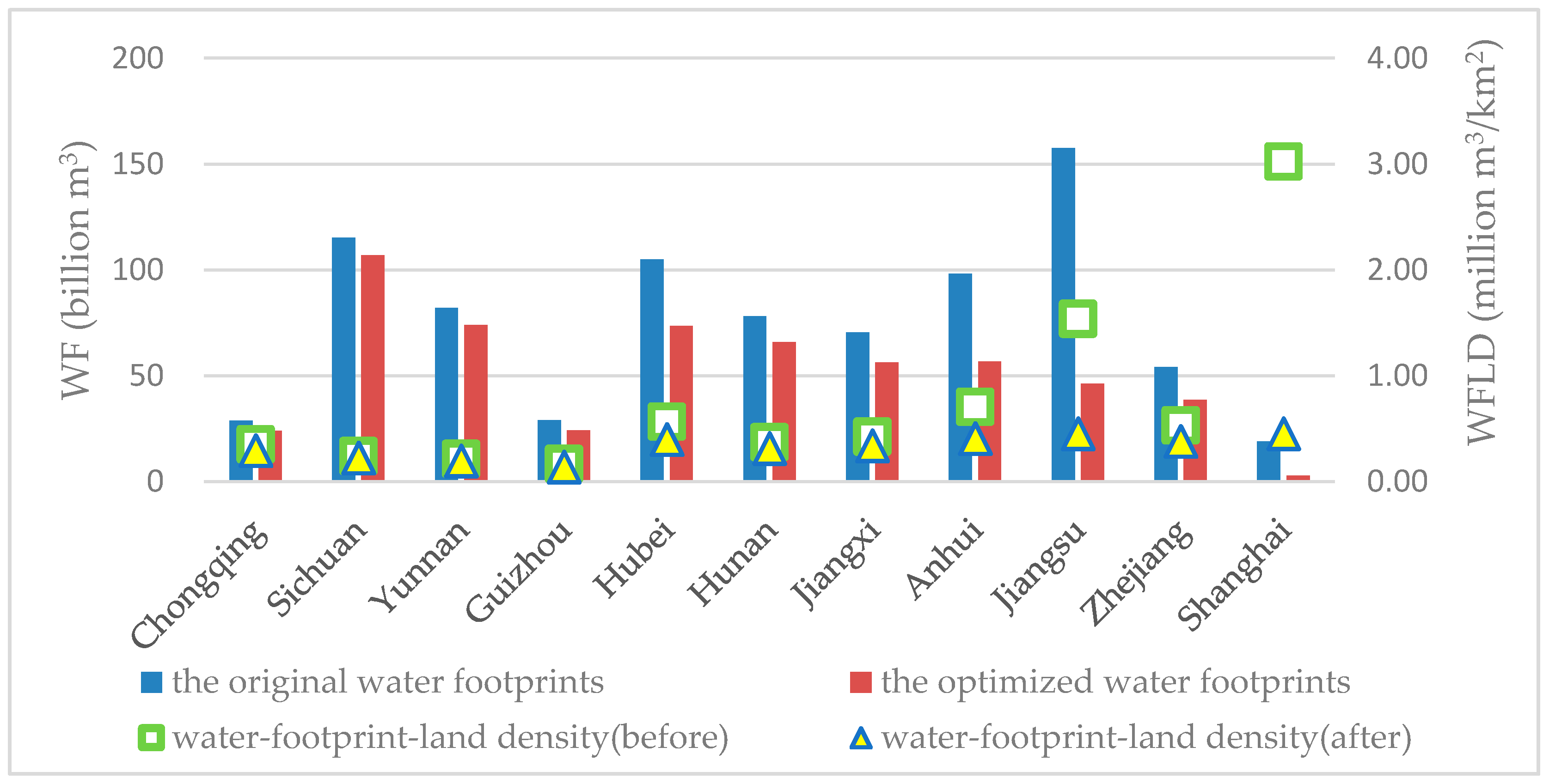
4.2. The Impact of Land Area on Water Resources Allocation

To characterize the influence of land area on water resources allocation, we introduce a new scheme known as the water allocation under spatial equity, which is determined by ( total   water   supply ) × optimized   water   footprints original   water   footprints . Based on the management practice in China, the total water supply equals the total water consumption for an area. Table 5 shows the result of water resource allocation under spatial equity based on the lexicographic optimization algorithm as well as WFLD.
By using the total water consumption data in 2013 in Table 1 and the optimized and original water footprints in Table 4, one can derive the optimal water resource allocation under spatial equity as given in the second column of Table 5. The original WFLD in the third column of Table 5 is determined as the ratio of the original water footprints in the second column of Table 4 and the corresponding land area in the second column of Table 1 and the optimized WFLD in the fourth column of Table 5 can be obtained in the same fashion.
Figure 4 shows the comparison between the optimized and the original total water footprints (the sum of agricultural and non-agricultural water footprints) as well as WFLD before and after optimization in the YREB.
As shown in Table 4 and Figure 4, optimized water footprints in the 11 YREB provinces decrease from the original values with an aggregate reduction of 32.04%. After optimization, across the 11 YREB provinces, the average WFLD decreases from 0.74 million m3/km2 to 0.33 million m3/km2, which indicates that the LABW scheme can achieve the goal of reducing water consumption per unit land area in the YREB. In addition, the standard deviation of WFLD across the 11 provinces is reduced from 0.85 million m3/km2 to 0.11 million m3/km2 after optimization, which clearly shows that the LABW solution can improve the fairness of water resource allocation in the YREB from a land area perspective.
Next, we take a closer look at the implied changes in total water footprints and WFLD in the YREB area based on the LABW scheme. On the one hand, from Table 4, we can see that the ratio of the optimized total water footprints of the four provinces in the upstream region, the three provinces in the midstream region, and the four provinces in the downstream region is approximately 10:9:6 and the ratio of the declines in the total water footprints after optimization is about 10:22:55. Given that the ratio of the total land area of the three segments is about 10:5:3, this result indicates that, by dramatically decreasing water footprints in the downstream and midstream regions, the LABW solution can properly consider the different land area endowments in the YREB and incorporate their impact on the allocation of water resources. On the other hand, after LABW optimization, it can be seen from Table 5 that the ratio of the average WFLD of the upstream, midstream, and downstream regions is about 3:5:6 while the corresponding ratio of the average WFLD reduction is 10:17:45. This shows a clear correlation with the ratio of the total land area. The larger the total land area, the smaller the average WFLD and its reduction ratio. Comparing the WFLD of each province before and after optimization, one can see that WFLD in Shanghai has the largest decline from the 3.02 million m3/km2 to 0.45 million m3/km2 and the WFLD in Sichuan has the smallest decline from 0.24 million m3/km2 to 0.22 million m3/km2. Given that the land area ratio between Shanghai and Sichuan is 63:4814 (Table 1), this result shows that WFLD can properly incorporate the influence of land area into equitable water resource allocation in the YREB.

5. Discussions

5.1. An Analysis of the Proposed Lexicographic Minimax Optimal Allocation Scheme

As previously stated, by applying the LABW optimization in this article, one can see from the bar charts in Figure 2, Figure 3 and Figure 4 that agricultural, non-agricultural, and total water footprints are all reduced from the original levels. According to the WFLD data in Table 5, the LABW scheme also reduces the water consumption per unit land area across the YREB. Compared with the original values in Table 5, LABW provides a more equitable allocation scheme of water resources from the perspective of ensuring development potentials of the unit land area. Since LABW uses available water resources as a constraint, the resulting solution guarantees a sustainable allocation scheme for YREB water resources management. On the other hand, given the significant differences in resource endowments and development levels among the 11 YREB provinces, it is a critical issue to examine how the LABW scheme can be possibly implemented in practice. Next, we shall analyze the LABW allocation of water resources in the YREB from a regional developmental perspective.
Water resources are the basic needs for human production and living activities. The consumption of water resources is closely linked to the regional development level such as population and GDP under the current water use pattern and technology. A closer examination of the population and economic output of the unit land area in each YREB province shows that the intensity of human production and living activities (as reflected in population and GDP) has a positive correlation with the WFLD (see the relevant data in Table 1 and Table 5). For example, in the four upstream provinces (Chongqing, Sichuan, Yunnan, and Guizhou), Chongqing has the highest WFLD of 0.35 million m3/km2 before optimization and 0.29 million m3/km2 after optimization (Table 5). In parallel, Chongqing’s population and GDP per unit land area are, respectively, 360.87 persons/km2 (calculated by the population and land area data given in Table 1) and 15.38 million RMB/km2 (calculated by the GDP and land area data given in Table 1). For these three indices, Chongqing scores the highest in the four upstream provinces. Similarly, Hubei in the midstream region and Shanghai in the downstream region demonstrate the same pattern. The highest original and optimized WFLD corresponds to the highest population density and GDP per unit land area in the midstream and downstream regions, respectively (See the last two columns in Table 5). In addition, WFLD reflects water consumption per unit land area and, to a certain degree, indicates its regional development level. As such, it can be employed to characterize the fairness of water resource allocation. Understandably, the smaller the standard deviation of WFLD, the more equitable the water resource allocation scheme is relative to the level of regional development. After LABW optimization, the standard deviation of WFLD across the YREB is reduced from 0.85 million m3/km2 to 0.11 million m3/km2. The WFLD in the upstream region has the smallest decline while the midstream and downstream regions have a more modest change and the largest decline in WFLD, respectively. This is due to the fact that the midstream and downstream YREB provinces have higher original WFLD values. To achieve more consistent WFLDs across the YREB, the downstream provinces such as Shanghai and Jiangsu have to dramatically reduce their WFLDs to achieve a more equitable allocation of water resources in the YREB.
In summary, the LABW optimal scheme can effectively reduce agricultural, non-agricultural, and total water footprints as well as achieve higher fairness in water resource allocation to make it more consistent with of the corresponding regional development levels in the YREB. Next, we shall analyze how different types of agricultural and non-agricultural land uses affect water resource allocation under LABW optimization.

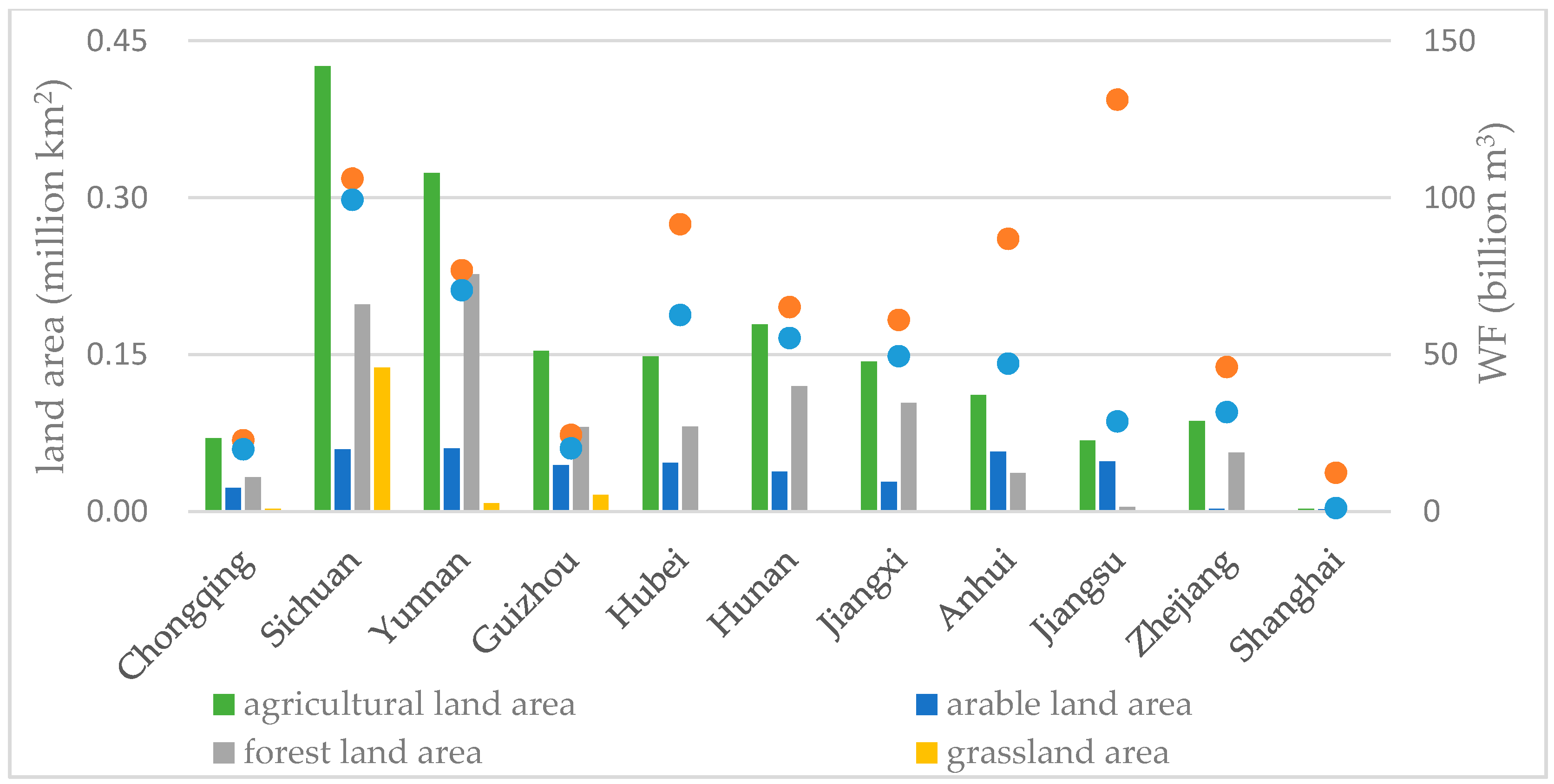
5.2. Analysis of Different Agricultural Land Uses’ Contribution to Water Footprints

It is well known that different land use types directly affect the regional industrial structure, which affects the relationship of the water supply and demand. By following China’s “Land Use Master Plan (2006~2020)” in the YREB promulgated by the provincial governments, this paper divides land uses into three types including agricultural, non-agricultural (construction), and unused land. Given that unused land does not generate water footprints, this paper optimizes agricultural and non-agricultural water footprints of the 11 YREB provinces based on their agricultural and non-agricultural land uses, respectively. The purpose of this categorization is to better understand how different land uses affect the allocation of water resources in the YREB.
Overall, Table A3 in Appendix C shows that the dominant land-use type in the YREB is agricultural land accounting for 84.01% of the total land area, which significantly contributes to the spatial heterogeneity in water footprints of the 11 YREB provinces. As reflected in the proportions of agricultural land relative to total land in different YREB provinces, their urbanization levels follow an increasing trend from upstream to midstream regions and, then, downstream. Comparing agricultural water footprints before and after optimization in the scatter plots in Figure 5, we can see that all 11 provinces experience a decline, but there exists a significant spatial difference in the magnitude. In general, the four upstream provinces on the left in Figure 5 experience the smallest decline followed by the next three midstream provinces in the middle in Figure 5 and, then, the rightmost four downstream provinces in Figure 5 with the largest declines. The optimized agricultural water footprints show a strong positive correlation with the agricultural land area of the 11 provinces with a correlation coefficient of 0.899, which increases from 0.425 before optimization. This shows that the lexicographic minimax allocation scheme puts a reasonable restriction on the agricultural water footprints and contributes to the spatial distribution of agricultural water resources. Although the amount of optimized agricultural water footprints varies significantly across the 11 provinces, their proportions relative to the total optimized water footprints in each province show a remarkable consistency with a small standard deviation of 0.161. This indicates that this allocation scheme helps to ensure spatial equity from a land area perspective. Next, given agricultural land’s significant contribution to water footprints, we further analyze how different agricultural land-use types contribute to spatial heterogeneity of provincial agricultural water footprints (Figure 5).
Table A3 in Appendix C shows that the majority of agricultural land in the YREB is forestry land (54.90%), which is followed by arable land (23.88%) and, then, grassland (9.67%). Therefore, this paper selects these three types of agricultural land to analyze their impact on agricultural water footprints in the YREB. Table A3 clearly shows the significant spatial heterogeneity in the distribution of the three types of agricultural land in the YREB. The proportions of arable land relative to agricultural land in the upstream, midstream, and downstream regions stand at 19.21%, 23.96%, and 40.67%, respectively. The ratios of grassland to agricultural land of the three segments in the YREB are 16.81%, 0.33%, and 0.13%, respectively, and the ratios of forestry land to agricultural land are 55.30%, 64.77%, and 36.18%, respectively. It is clear from these statistics that downstream provinces have the highest proportions of arable land. Forestry land is mainly located in the upstream and midstream regions as well as Zhejiang in the downstream region. The grassland area is primarily distributed in the upstream region especially in Sichuan. In general, the contribution of different types of agricultural land to agricultural water footprints differs significantly. Taking Sichuan as a representative example since it has significant portions of forestry land, arable land, and grassland, we can examine their different contributions to agricultural water footprints. According to Equation (1), the WFLD of forestry land, arable land, and grassland in Sichuan can be calculated as 0.092 million m3/km2, 0.73 million m3/km2, and 0.53 million m3/km2. It clearly shows that each unit of arable land consumes more water than that of grassland and each unit of grassland requires more water than that of forestry land. Given YREB’s significant proportion of forestry land with low WFLD, a negligible proportion of grassland with moderate WFLD, and a good proportion of arable land with high WFLD, it can be deduced that arable land is the main contributor of YREB’s agricultural water footprints. This is consistent with the fact that the 9 YREB provinces except for Shanghai and Guizhou are the main grain producers in China.
Table 1 indicates that water resources in the upstream tend to be abundant and account for 49.03% of the total in the YREB. On the other hand, although the upstream claims 55.09% of the total YREB land area, its land suffers severe rocky desertification and soil erosion. The area of rocky desertification in the upstream region accounts for 62.5% [34] of the total amount in China and significantly reduces available land for agricultural development and cultivation. In addition, as per a survey conducted by China’s State Forestry Administration on the upstream of YREB in 2012, its agricultural activities further aggravate the situation of rocky land desertification in certain areas of the Yunnan-Guizhou Plateau and the Sichuan Province. This serious issue has threatened the ecological security of the upstream region. At the same time, the hilly landscape in the upstream region leads to fragmented arable land with low efficiency and coverage of farmland irrigation as well as diseconomies of scale. Furthermore, the survey also reveals that artificial afforestation and grass planting can significantly reverse land rocky desertification with a contribution rate as high as 72%. Given that the upstream ecological security is not only critical to sustainable development of the four upstream provinces but also furnishes the bottom line for the entire YREB, it is essential to contain rocky desertification in the upstream region by controlling its arable land area and enhancing afforestation and grass planting. In view of the characteristics of upstream landscapes, rocky desertification status, and water resources endowment, the recommended modest decline of agricultural water footprints in the upstream region can be achieved by implementing the following changes. First, cultivable instead of total land area should be considered as an indicator to allocate water resources in the YREB, which helps reduce water resource consumption in the upstream. Second, it is proposed to integrate water resource allocation with the national project of Grain for Green and carry out comprehensive, small watershed treatment projects in the upstream region. As such, we can prioritize water uses for afforestation and grassland, which not only helps to combat rocky desertification but reduces water consumption per unit land area. Third, current energy uses in the upstream rural area heavily depend on firewood, which contributes to deforestation and rocky desertification. We suggest adjusting the structure of rural energy uses by promoting small-scale rural biogas programs, which improves ecological security and enhances the carrying capacity of regional water and land resources in the upstream region. Lastly, given the fragmented nature of arable land in the upstream, it is generally impossible to exploit economies of scale in agricultural cultivation. As such, across the upstream, agricultural production should be planned as basic self-sufficiency supplemented by the appropriate import. In severely rocky desertification areas, it is recommended to relocate these rural residents to more habitable places by offering skill training and other incentives. By incorporating the previously mentioned measures, the modest reduction in agricultural water footprints in the upstream region is attainable and the ecological security of the upstream region as well as the entire YREB will be improved.
Table 1 shows that the three midstream provinces account for 34.40% and 27.70% of the total amount of water resources and land area in the YREB, respectively. In general, rocky desertification is much milder and agricultural land is much flatter in the midstream, which makes its water resources more compatible with its land resources. On the one hand, since the three midstream provinces are all major agricultural provinces, many years of land reclamation from lakes and prevalent pen culture have significantly affected the flood discharge capacity of the waterway system, which results in frequent flooding and high economic loss in the midstream area. According to the data released by the Chinese Ministry of Water Resources [35], during the period from 2013 to 2016, the area affected by flood in the three midstream provinces increased from 11,769.5 km2 to 29,662.2 km2. The percentage of the land area affected by flood is 3.12% in the midstream region during this period while the corresponding ratios are 1.94% and 0.86% for the whole YREB and across China, respectively. Given the characteristics of the agricultural land, we propose the following strategies to achieve the moderate agricultural WF reduction in the midstream area. The first measure is to enforce the project of returning farmland to lakes so that the smooth flow of waterways can be restored in the midstream river and lake networks. In so doing, the area of arable land will be shrunk, which curbs agricultural water footprints. In addition, the improved waterway system will reduce flooding risk, which enhances agricultural production and safety. The second strategy is to improve the efficiency of water and land resource utilization by changing the planting structure of the main crops (for instance, shifting from the current indica-type rice to high-quality grain and oil crops such as super rice and double-low rapeseed) and by upgrading the agricultural cultivation from fragmented and labor-intensive to a more integrated and mechanized production mode.
From Table 1, one can tell that the available water resources and land area in the four downstream provinces account for 16.57% and 17.20% of the corresponding total area across the YREB. The downstream region faces the situation of a limited water supply and more arable land. Another significant issue is heavy pollution. The LABW optimal solution demands significant reduction in agricultural water footprints in each of the four downstream provinces especially Shanghai and Jiangsu. This solution reflects the current over-exploitation and unsustainable development of water and land resources in the downstream region. Except for Zhejiang, which has a significant proportion of forestry land, the other three downstream provinces have good proportions of arable land, which is not subject to land rocky desertification and consists of large areas of flat or gently rolling land. Anhui and Jiangsu are important grain production bases and Shanghai is the largest industrial municipality in China. Intense human production and living activities in the downstream region require a larger share of the total population and GDP in the whole YREB, accounting for 37.62% and 52.93%, respectively. A severe shortage of water resources exists in the downstream region. In 2013, the annual per capita water resources of the four downstream provinces in the downstream are 835.56 m3/year and the corresponding annual quotas are as long as 115.93 m3 and 357.08 m3 in Shanghai and Jiangsu, respectively (Table 1). According to the Falkenmark’s water-stress index [25,26], annual per capita water resource possession of 500–1000 m3 is categorized as a severe water shortage and a value below 500 m3 is treated as an extreme water shortage. Based on this standard, the downstream region as a whole is a severe water shortage area while Jiangsu and Shanghai are extreme water shortage areas.
In addition to the scarcity of water resources in the downstream area, its intense industrial and agricultural activities also beget severe water pollution problems. In recent years, the total annual wastewater discharge in the downstream averages at about 15 billion tons and accounts for about 50% of the total wastewater discharge in the YREB [36]. Purification of wastewater requires consumption of additional scarce water resources. Therefore, wastewater discharge further intensifies the water resource shortage situation in the downstream.
Given this scenario, the following two strategies are recommended to reduce agricultural water footprints and implement the optimal allocation of water resources in the downstream. The first strategy is to improve the efficiency of water and land resource utilization. Take Shanghai as an example. It is one of the most developed municipalities and serves as an important financial center and economic powerhouse in China. Its agricultural land accounts for 40.85% of its total land (Table A3 in Appendix C) and takes a minor role in its economic development. To effectively contain its agricultural water footprints, it is recommended that agricultural residents be offered job skill trainings and migrated to the urban area so that more agricultural land can be converted to industrial uses, which improves utilization efficiency of limited water and land resources in Shanghai. As for Jiangsu, it is the largest grain producer in the downstream. Jiangsu is characterized by abundant transit water resources passing through its jurisdiction, but its allocation is very limited, which makes it one of the extreme water shortage provinces in the YREB. However, due to a lack of a proper water property rights ascertaining mechanism and lax enforcing of penal codes for water resources overexploitation, local residents are typically unaware of the current situation of the water shortage and have been historically over-withdrawing transit water resources. Its irrigation system is dominated by a low-efficient canal mode. At the same time, Jiangsu mainly produces rice, vegetables, and other high-water-consumption crops, which results in high agricultural water footprints. Therefore, to achieve effective reduction in Jiangsu’s agricultural water footprints, sensible suggestions are to shift from current canal flood irrigation to sprinkler and drip irrigation, change its cultivation structure to low-water-consumption crops, educate farmers about water rights and encourage water conservation, and ascertain water property rights and implement water rights trading among different users. The second strategy is to closely monitor and strictly control agricultural water pollution. By taking advantage of the current stricter enforcement of environmental protection laws and regulations, we recommend promoting the newly-introduced river chief system, implementing the most stringent water resources management practices, and carrying out the “beautiful rural construction” project. It is also necessary to improve the water quality of key lakes such as Taihu, Hung-tse, and Luoma Lake, which would enhance the carrying capacity of the water environment in the downstream region. Furthermore, it is important to vigorously carry out a comprehensive improvement of the rural environment, promote soil testing and a fertilizer recommendation, and control agricultural non-point source pollution, which would reduce agricultural pollution emissions.
In conclusion, given the different reduction targets and specific agricultural land use characteristics in the three YREB segments, we recommend distinct strategies to implement the recommended optimal allocation schemes. More specifically, the upstream area is recommended to use cultivable land as an indicator to allocate water resources, prioritize a water supply for afforestation and grassland, adjust the rural energy structure, and import agricultural products as needed. The midstream provinces are expected for implementing the project of returning farmland to lakes, upgrading the waterway system, and changing the planting structure. The downstream region can achieve the reduction target by improving the utilization efficiency of water and land resources and controlling agricultural water pollution.

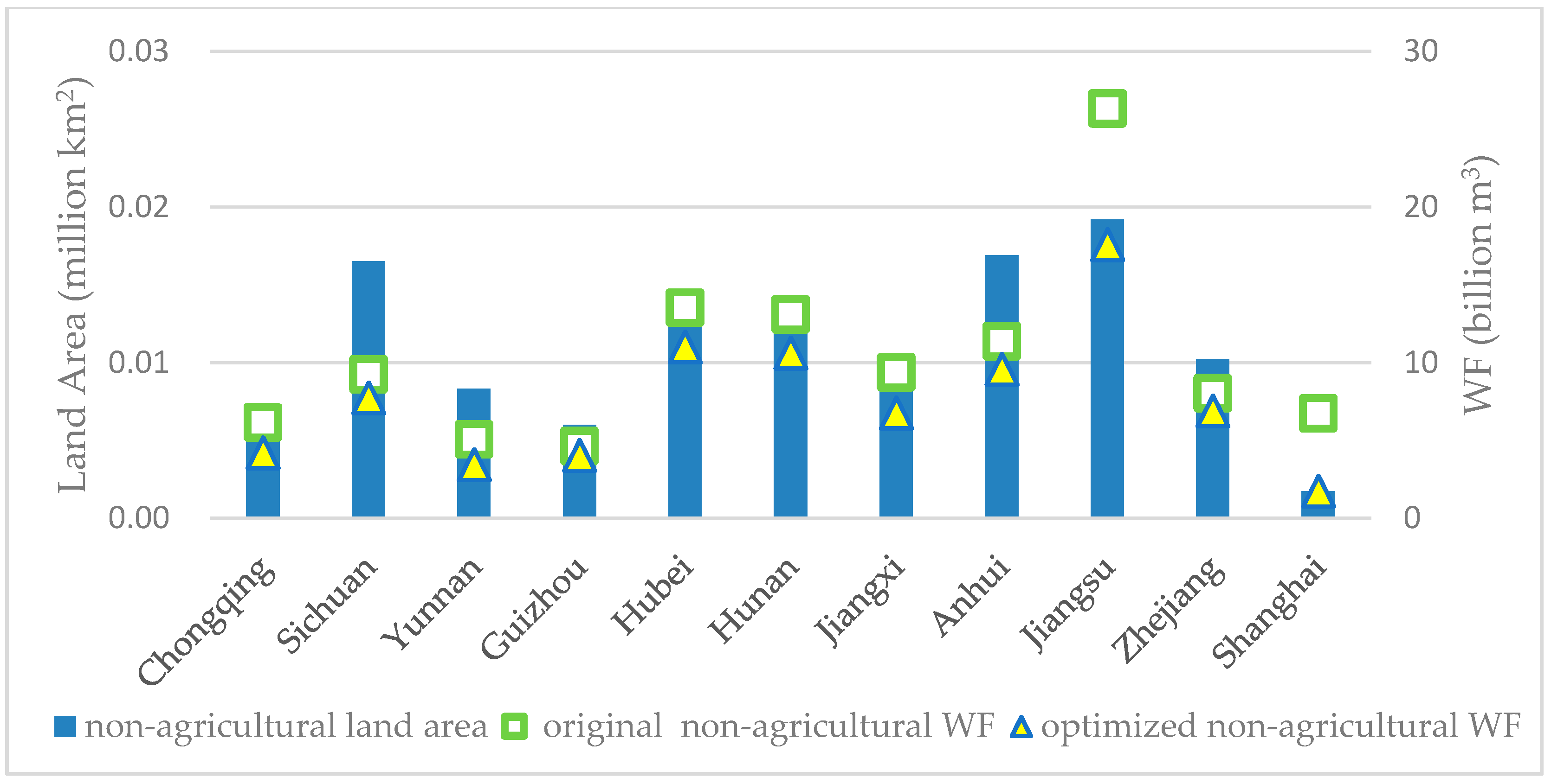
5.3. An Analysis of Non-Agricultural Land’s Contribution to Water Footprints

Figure 6 illustrates how non-agricultural water footprints change after the optimal allocation scheme is applied for non-agricultural land.
As shown in Figure 6 and Table A3, non-agricultural land accounts for 3.30%, 6.73%, and 13.71% of the total land in the upstream, midstream, and downstream regions in the YREB, respectively. This is in line with the average rate of urbanization of the three segments in the YREB (45.39%, 50.45%, 66.39%, respectively) as well as the distribution of non-agricultural water footprints across the whole area. It confirms that the larger the non-agricultural land area in a region is, the higher the urbanization rate is and the higher water consumption is due to industrial production, urban residents, and service industries. As shown in Equation (2), non-agricultural water footprints consist of industrial water footprints, domestic water consumption, and urban greening coverage. Table A2 shows that, before optimization, the total industrial water footprints in the upstream, the midstream, and the downstream regions in the YREB are 14.577 billion m3, 24.501 billion m3, and 36.034 billion m3, respectively, accounting for 58.01%, 68.00%, and 68.62% of the total non-agricultural water footprints in the corresponding segment. Similarly, the data in Table A2 illustrate that domestic water consumption accounts for 38.88%, 30.50%, and 28.93% and urban greening takes up 3.10%, 1.50%, and 2.46% of the non-agricultural water footprints in the upstream, midstream, and downstream segments, respectively. It is clear that, across the whole YREB area, industrial production is the main contributor of non-agricultural water footprints, which is followed by domestic water consumption and, then, urban greening coverage for urban afforestation. Therefore, to effectively contain non-agricultural water footprints and implement the LABW optimal scheme, we should focus on introducing proper measures to reduce industrial water footprints and domestic water consumption.
As shown in Figure 3, the LABW optimal allocation requires all 11 YREB provinces to reduce their non-agricultural water footprints at different levels. In terms of the percentage decline, the highest reduction is 74.06% for Shanghai. Chongqing, Yunnan, Jiangxi, and Jiangsu are required to achieve a middle-range decline of 31.19% on average. The other provinces known as Sichuan, Guizhou, Hubei, Hunan, Anhui, and Zhejiang should aim at a moderate decrease of 16.04% on average. As mentioned before, Table A2 shows that the industrial production and domestic water consumption are the main contributors of non-agricultural water footprints. As such, we shall discuss countermeasures for reducing non-agricultural water footprints from these two aspects by examining the characteristics of water and land resource endowments and the industrial structure in the YREB.
First, the highest decline in non-agricultural water footprints before and after the LABW optimization in Shanghai is mainly ascribed to the scarcity of its non-agricultural land and water resources. The supply and demand equation in Shanghai poses a significant challenge for water resources managers. On the one hand, Shanghai has the highest urbanization rate in the 11 YREB provinces, which reached 89.60%. It is not only an international financial center but also a major industrial powerhouse in China. Its leading industries [37] such as medicine, automobile, tobacco, petrochemical, and other industries tend to be water-intensive. Its dense urban population and highly-developed industrial economy lead to strong demand for industrial and urban domestic water demand. On the other hand, from the supply side, Shanghai has limited available water resources and has historically been over-withdrawing water resources from the Yangtze River beyond its allocated quota to meet industrial production and urban domestic water demand. Given that Shanghai’s construction land area only accounts for 1.41% of the total in the YREB (Table A3 in Appendix C), it is natural that the LABW optimization requires a significant reduction in Shanghai’s non-agricultural water footprints from its current level. As the largest and highly industrialized municipality in China, Shanghai has a similar situation with Singapore [38]. Both face severe mismatch of water supply and demand. As such, it is suggested that Shanghai learn from the success story of Singapore. Its extensive use of seawater desalination and wastewater reuse has effectively alleviated the water shortage issue. Singapore even expects to achieve water resources self-sufficiency by 2061. Given Shanghai’s geographical location and economic strength, it can resort to seawater desalination and wastewater reuse technologies to reduce its use of water resources in the Yangtze River, which achieves the LABW reduction goal. This strategy is economically sensible. The “2016 National Seawater Utilization Report” [39] promulgated by the State Oceanic Administration points out that the cost of seawater desalination typically stands at 5-8 RMB/ton and some plants can achieve as low as 4–5 RMB/ton. In the same year, the comprehensive water price for industrial use in Shanghai is about 5 RMB/ton [40]. By tapping into its technological and economic strengths and pursuing seawater desalination and wastewater reuse, Shanghai can open up new water sources to meet its demand and effectively reduce its non-agricultural water footprints.
Second, the LABW optimal solution requires a middle-range reduction of non-agricultural water footprints in Chongqing, Yunnan, Jiangxi, and Jiangsu. This result is consistent with their non-agricultural land area and the current non-agricultural water footprints. Given that the two main contributors to non-agricultural water footprints are industrial production and urban domestic water uses, the key to achieving the recommended reduction is to optimize the industrial structure and control the urban population. By examining these four provinces’ industrial structures, one can see that Chongqing’s strengths are modern manufacturing while Yunnan and Jiangxi focus on primary product processing and Jiangsu is characterized by a more comprehensive range of manufacturing industries. According to the blueprint “Made in China 2025” [41], China aims to enhance the digital, networking, and intelligent levels of her manufacturing industry and improve the efficiency of resource utilization. Given the current reality and this general policy environment, for Chongqing and Jiangsu, it is recommended that they take advantage of this opportunity to develop intelligent manufacturing and a cross-regional industrial chain, capitalize on the Yangtze River marine shipping channel, and improve the efficiency of water and land resource utilization, which reduces their non-agricultural water footprints. For Yunnan and Jiangxi, they are suggested to take advantage of their scenic landscape and ecosystem as well as cultural attractions to develop eco-tourism and cultural and creative industries. They are also encouraged to foster further processing of primary products by cross-regional industrial chain integration, which effectively reduces their non-agricultural water footprints.
Third, for those provinces with moderate reductions in non-agricultural water footprints as per LABW optimization, Guizhou has the lowest current non-agricultural water footprint, which corresponds to its relatively small non-agricultural land area. While the other five provinces (Sichuan, Hubei, Hunan, Anhui, and Zhejiang) tend to have a larger non-agricultural land area and higher original non-agricultural water footprints. A quick survey of the industrial structures of these six provinces reveals that their main industries are in manufacturing and primary product processing. Therefore, our first recommendation is to take advantage of the “Made in China 2025” incentives to promote intelligent manufacturing, enhance cross-regional industrial chain integration, and improve land and water use efficiency, which reduces non-agricultural water footprints. In addition, Zhejiang is identified as a good role model for other provinces. Its non-agricultural land area is relatively large, but it has been taking measures to control its non-agricultural water footprints. As a result, the required reduction by LABW is quite modest. By examining the current practices in Zhejiang, we note that it has embarked on a sustainable development path of putting ecology and green development first. This has been accomplished by constructing a green manufacturing system, promoting water conservation, and implementing eco-compensation. A key lesson that can be extended to other provinces in reducing their non-agricultural water footprints is to foster a social consensus on “ecology and green development first” by active publicity and education to the public.
In short, based on different reduction levels of non-agricultural water footprints in the 11 YREB provinces, we categorize them into the three groups mentioned above. For the jurisdiction that requires the highest reduction, Shanghai can achieve its goal by reducing the cost of its critical infrastructure operations [42] and resorting to seawater desalination and wastewater reuse technologies. The four provinces with less water stress can reach their 31.19% decline target by optimizing their industrial structure and controlling their urban population. The six provinces with the least pressure on non-agricultural water resources are recommended to promote intelligent manufacturing, strengthen water resources publicity and education, and foster the “ecological and green development priority” social consensus.

6. Conclusions

This paper employs a lexicographic optimization algorithm to allocate basin water footprints with agricultural and non-agricultural land area as the influencing factor, respectively. The key contribution is to introduce the water footprint theory into the allocation process with a purpose of balancing the water supply and demand. Next, based on the 2013 sectional data of the 11 YREB provinces, we perform a cross-scale analysis and categorization of land uses for lexicographic allocation of basin water footprints. This case study shows that, (1) for each YREB province, its optimized agricultural and non-agricultural water footprints decrease from the current levels with a heterogeneous pattern across the area; (2) The optimal allocation scheme leads to a lower WFLD for each of the 11 YREB provinces with the largest decline in Shanghai and the smallest decline in Sichuan; (3) For agricultural water footprint allocation, the land use structure across the three land types including arable land, forest land, and grassland is the main contributor to the spatial heterogeneity of the optimized agricultural water footprints in the upstream, midstream, and downstream areas in the YREB; (4) For non-agricultural water footprints, the main contributor to the spatial heterogeneity lies in the difference in regional industrial structures on top of the non-agricultural land area. The contributions are threefold. First, this research furnishes a proper accounting of the current agricultural and non-agricultural water footprints in the YREB based on the 2013 data. Second, based on the proposed lexicographic minimax algorithm, optimal allocations of agricultural and non-agricultural water resources are obtained for the 11 YREB provinces by using the land area as the influencing factor. Third, proper policy changes are put forward to implement the optimal allocation schemes and reduce agricultural and non-agricultural water footprints after examining the specific water and land endowments as well as the agricultural and industrial structures in the 11 YREB provinces. This research reveals that a successful implementation of the recommended optimal allocation scheme can achieve an aggregate water footprint reduction by 32.04% across the YREB where agricultural water footprints are reduced by 32.93% and non-agricultural water footprints are required to decrease by 26.34%. By following the policy change recommendations and achieving these reduction goals, the water resource shortage pressure will be effectively alleviated and more balanced and sustainable development can be expected in the YREB.
This study can be further extended along several different directions. First, grey water footprints are not accounted for given the unavailability of reliable data. Second, the FAO crop coefficient data are used to determine agricultural water footprints since region-specific data are difficult to obtain for local crops in the YREB. Third, for the sake of convenience, we do not consider the differences in water consumption behavior in different industries. Last, this research adopts the land area as the single influencing factor in allocating water resources. Other factors such as population and GDP should also be considered so that a more balanced allocation scheme can be obtained. These issues warrant further research.

Author Contributions

All authors make significant contributions to this article. Conceptualization, G.L. Formal analysis, G.L., L.S., and K.W.L. Funding acquisition, G.L. Investigation, L.S. Methodology, G.L. Supervision, G.L. and K.W.L. Writing—original draft, G.L. and L.S. Writing—review & editing, G.L., L.S., and K.W.L.

Funding

This research was supported by the National Key Research and Development Project of China (2017YFC0404600), the National Social Science Foundation of China (No. 14CGL030), and the National Natural Science Foundation of China (No. 71433003, 71572040, 41501580).

Conflicts of Interest

The authors declare no conflict of interest.

Appendix A. Lexicographic Algorithm

To solve Model (3), the lexicographic algorithm in Liu et al. (2012) [43] is employed. To make the paper self-contained, the algorithm therein is replicated below.
To describe the lexicographic minimax solution process, the following two definitions are needed.
Definition 1
[17]. For two vectors α = ( α 1 , α 2 , , α m ) and β = ( β 1 , β 2 , , β m ) , if there exists a positive integer k, 1 k m , such that α i = β i for any 1 i < k , and α k < β k , then vector α is strictly less than β in a lexicographic order denoted by α < L β . Similarly, a weak lexicographic order α L β is defined as α < L β or α = β .
Definition 2
[17]. If a non-increasing lexicographic solution vector x = ( x 1 , x 2 , , x n ) is less than or equal to any other feasible configuration solution, then the feasible configuration solution x + n is called the lexicographic minimax solution.
The key to tackling a Leximinimax problem is to solve the following minimax problem successively by using the lexicographic method.
P = min [ max i I ( α i f ( x i ) ) ] s . t . i I α i f ( x i ) Q i , i I L i f ( x i ) U i , i I
The algorithm presented next follows the basic idea in References [17,21,44]. Their original concern is to address resource allocation in producing multiple products. In this paper, fair allocation of provincial water footprints under limited water supply constraints can be characterized as a single resource allocation in a single period with multiple stakeholders. Luss’s algorithm is a handy tool to solve our problem. However, because water footprints are shared resources, the solution process of our lexicographic minimax allocation differs from the traditional algorithm in the following aspects.
(1)
Assumptions: Due to the difference between production resources (e.g., capital and human resources) and natural resources (e.g., land and water resources), traditional industrial production lexicographic minimax problems typically employ cumulative variables while this paper uses piecewise continuous variables.
(2)
Decision variables: In the traditional algorithm, decision variables are production quantities, which consume limited resources in the production process and are suitable for enterprise production planning. On the other hand, decision variables in this paper are water footprints, which are appropriate for allocating provincial water resources under government regulation and market mechanisms.
(3)
Solution procedure: The original solution procedure mainly uses constraints to internalize multiple resources and aims to solve the lexicographic minimax problem with multiple subjects and multiple periods. Given that our decision variables are water footprints, the algorithm in this paper is designed for lexicographic minimax problems for a single limited resource with multiple subjects.
This paper enhances the applicability of the traditional algorithm by adapting it to handle equitable allocation of provincial water footprints with a single shared resource. Next, the procedure to solve the proposed lexicographic minimax model can be described as follows.
Step 0: Initialize: L i = L i and U i = U i for all i I .
Step 1: Compute:
S i = i I ( x i Q i ) , i I
R i = i I ( W F i / α i ) , i I
For province i’s available water quantity Qi, remove all i’s such that S i 0 .
If all Q i = 0 , let x i = W F i , i I , then k = 0 , go to Step 8.
Step 2: Calculate:
T i = i W F i a , i I
M i = L A i L A i × W F i , i I
a v g i = a L A i , i I
k i = T i / R i , i I . For R i > 0 , let k = max { k i } .
Step 3: Determine: x i = x i ( 1 k / α i ) , i I .
Step 4: If W F i × ( 1 k / α i ) MIN ( W F i , M i ) , i I , let x i = MIN ( W F i , M i ) , i I .
Step 5: If MIN ( W F i , M i ) a v g i × L A i , i I , go to Step 6, else go to Step 7.
Step 6: If W F i × ( 1 k / α i ) 0 , i I , let x i = MIN ( W F i , M i ) , i I .
Step 7: If W F i × ( 1 k / α i ) a v g i × L A i , i I , let x i = a v g i × L A i , i I .
Step 8: For the minimax problem in each iteration, perform the following calculation:
x i = W F i f o r a l l i I , Q i = 0 ;
P = max [ k , max i ( α i f ( x i ) ) ] .
Step 9: Adjust Qi according to the minmax problem result during the previous iteration and remove i’s such that i { i : | R i = 0 } .
Step 10: Update constraints L ˜ i and U ˜ i ,
Remove i’s such that i { i : | L ˜ i = U ˜ i } , update Q i .
Remove i { i : | L ˜ i = Q i } . If all i’s have been removed, stop.
Otherwise, define a new P* problem with remaining i I and go back to Step 0.

Appendix B. Raw Data for Water Footprint Accounting

The tables below show the data of agricultural and non-agricultural water footprints of the 11 provinces and municipalities in the YREB. Table A1 shows the raw data and final calculation agricultural water footprints including cultivated crops and livestock husbandry water footprints. Table A2 shows the data of non-agricultural water footprints, which consist of industrial, domestic, and urban greening water footprints.
Table A1. The data for agricultural water footprints in the YREB (unit: 100 million m3).
ChongqingSichuanYunnanGuizhouHubeiHunanJiangxiAnhuiJiangsuZhejiangShanghai
Wheat3.9248.457.595.7752.101.390.34187.81214.763.530.00
Barley0.000.000.000.000.000.000.000.002.420.500.00
Broad bean0.000.000.000.000.000.000.000.001.881.240.00
Paddy58.36181.2953.4636.85231.38330.44284.5770.8480.7396.890.00
Maize16.7845.7453.5319.9719.4913.140.9134.9317.752.410.00
Sorghum0.140.000.000.000.000.000.000.000.000.000.00
Potato7.709.117.537.643.445.320.001.421.401.780.00
Soybean7.5510.133.871.343.760.006.4524.6213.174.9429.45
Cotton0.001.370.000.0054.3423.1315.4730.2324.323.390.49
Peanut2.3813.342.082.0010.835.5211.2523.499.421.630.00
Rapeseed7.3843.6912.0613.7426.0529.5814.3627.5726.627.440.36
Sesame0.006.110.000.0015.651.784.408.070.040.020.00
Sugarcane0.005.98204.3217.043.4812.018.150.000.830.000.00
Mint0.000.000.000.000.000.000.000.000.000.000.00
Vegetables21.24225.2642.2627.0149.7449.3725.650.00256.6532.047.17
Tobacco leaf0.000.959.760.790.791.240.250.210.000.020.00
Melon and fruit9.6626.5938.718.726.679.2211.3915.1089.0417.202.00
Tea leaf0.000.9246.040.540.000.000.000.640.000.000.00
Sum (cultivated crops)135.09618.93481.21141.41477.71482.13383.19424.94739.01173.0439.47
Livestock products
Pork40.16181.14166.5859.76168.11156.4688.29114.80125.2778.0911.12
Beef10.7458.3268.1721.0040.6611.8226.4236.568.3710.580.75
Lamb0.0023.4413.182.9615.360.661.5029.4117.2711.480.72
Poultry16.5082.290.0010.6060.290.0055.1796.37187.47121.4413.54
Honey0.530.950.110.050.550.000.360.490.132.410.00
Egg21.7872.3021.816.50146.360.0050.95124.91212.8753.416.83
Milk1.4619.8218.151.316.470.004.4541.1822.047.4350.57
Cocoon0.383.320.000.000.000.000.000.000.001.940.00
Sum (Livestock products)91.55441.57288.00102.17437.81168.94227.14443.72573.43286.7883.53
Sum (Agricultural WF)226.651060.50769.21243.58915.52651.07610.33868.661312.44459.83123.00
Table A2. The data for non-agricultural water footprints in the YREB (unit: 100 million m3).
ChongqingSichuanYunnanGuizhouHubeiHunanJiangxiAnhuiJiangsuZhejiangShanghai
Industrial output value
(100 million RMB)
5249.6511,471.573767.582686.5210,531.379996.68146437.9865892825,612.2316,368.437236.69
Industrial water consumption
(100 million m3)
36.744.724.627.790.287.761.391.223855.767.2
Product WF
(100 million m3)
36.744.724.627.790.287.761.392.723855.766.2
Import virtual water42.0630.524.1626.1846.1237.1949.1539.1846.1840.1934.19
Export virtual water37.1629.4619.4624.7542.1838.3246.1551.6376.1964.5359.15
Trade water footprint
(100 million m3)
4.91.044.71.433.94−1.133−12.45−30.01−24.34−24.96
Sum (Industrial WF)41.645.7429.329.1394.1486.5764.378.75207.9931.3642.24
Domestic water consumption19.142.519.516.640.741.827.430.952.843.824.4
Urban greening coverage0.94.220.70.62.72.14.22.75.20.8
Sum (Non-agricultural WF)61.692.4450.846.43135.44131.0793.8113.85263.4980.3667.44

Appendix C. Raw Data for Land Use Types

Table A3 below shows the data of land areas for different use types for the 11 provinces in the YREB.
Table A3. The data for land use types in the YREB (unit: km2).
ProvinceTotal LandAgricultural LandNon-Agricultural LandUnused Land
ArableForestryGrasslandGarden PlotOther Land
Chongqing82,30022,62732,73123792589959662266152
Sichuan481,40059,480197,894137,602811922,83616,50938,960
Yunnan383,30060,487226,9607739945319,056831251,293
Guizhou176,00044,38080,59015,913130711,400600016,410
Hubei185,90046,58081,042488445615,54914,33023,455
Hunan211,80037,873119,6671038497415,55614,03718,655
Jiangxi167,00028,253104,0253631577767961814,143
Anhui139,70057,18036,675338339113,99616,90011,220
Jiangsu102,60047,620413320315013,02519,19215,460
Zhejiang102,000258056,348314,08213,69310,2345061
Shanghai6300193611106546217321994

References

  1. UNESCO. The United Nations World Water Development Report 2017; UNESCO: Paris, France, 2017. [Google Scholar]
  2. Jerson, K.; Rafael, K. Water allocation for economic production in a semi-arid region. Int. J. Water Resour. Dev. 2002, 18, 391–407. [Google Scholar]
  3. Eleftheriadou, E.; Mylopoulos, Y. Game theoretical approach to conflict resolution in transboundary water resources management. J. Water Resour. Plan. Manag. 2008, 134, 466–473. [Google Scholar] [CrossRef]
  4. Liehr, S.; Röhrig, J.; Mehring, M.; Kluge, T. How the social-ecological systems concept can guide transdisciplinary research and implementation: Addressing water challenges in Central Northern Namibia. Sustainability 2017, 9, 1109. [Google Scholar] [CrossRef]
  5. Hoestra, A.Y. Virtual water trade: Proceedings of the international expert meeting on virtual water trade. In Value of Water Research Report Series No. 12; UNESCO-IHE Institute for Water Education: Delft, The Netherlands, 2003. [Google Scholar]
  6. Kampman, D.A.; Hoekstra, A.Y.; Krol, M.S. The Water Footprint of India; Value of Water Research Report Series (No. 32); UNESCO-IHE Institute for Water Education: Delft, The Netherlands, 2008. [Google Scholar]
  7. Van Oel, P.R.; Mekonnen, M.M.; Hoekstra, A.Y. The external water footprint of the Netherlands: Geographically—Explicit quantification and impact assessment. Ecol. Econ. 2009, 69, 82–92. [Google Scholar] [CrossRef]
  8. Chapagain, A.K.; Orr, S. UK Water Footprint: The Impact of the UK’s Food and Fibre Consumption on Global Water Resources; Godalming WWF-UK: Surrey, UK, 2008. [Google Scholar]
  9. Ma, D.; Xian, C.; Zhang, J.; Zhang, R.; Ouyang, Z. The evaluation of water footprints and sustainable water utilization in Beijing. Sustainability 2015, 7, 13206–13221. [Google Scholar] [CrossRef]
  10. Casolani, N.; Pattara, C.; Liberatore, L. Water and Carbon footprint perspective in Italian durum wheat production. Land Use Policy 2016, 58, 394–402. [Google Scholar] [CrossRef]
  11. Cartone, A.; Casolani, N.; Liberatore, L. Spatial analysis of grey water in Italian cereal crops production. Land Use Policy 2017, 97–106. [Google Scholar] [CrossRef]
  12. Salmoral, G.; Willaarts, B.; Garrido, A.; Guse, B. Fostering integrated land and water management approaches: Evaluating the water footprint of a Mediterranean basin under different agricultural land use scenarios. Land Use Policy 2017, 61, 24–39. [Google Scholar] [CrossRef]
  13. Sun, H.H.; Cheng, X.F.; Dai, M.Q.; Wang, X.; Kang, H.D. Study on the influence factors and evaluation indes system of regional flood disaster resilience based on DEMATEL method-taking ChaoHu Basin as a case. Resour. Environ. Yangtze Basin 2015, 24, 1577–1583. [Google Scholar]
  14. Dong, L.; Sun, C.Z.; Zou, W.; Xi, X. Assessment and spatial-temporal evolution of water consumption fairness from a water footprint perspective in China. Resour. Sci. 2014, 36, 1799–1809. [Google Scholar]
  15. UNESCAP. Principles and Practices of Water Allocation Among Water-Use Sectors; UNESCAP: Bangkok, Thailand, 2000. [Google Scholar]
  16. Mimi, Z.A.; Sawalhi, B.I. A decision tool for allocating the waters of the Jordan River basin between all riparian parties. Water Resour. Manag. 2003, 17, 447–461. [Google Scholar] [CrossRef]
  17. Luss, H. On equitable resource allocation problems: A lexicographic minimax approach. Oper. Res. Lett. 1999, 47, 361–376. [Google Scholar] [CrossRef]
  18. Ogryczak, W.; Śliwiński, T.; Wierzbicki, A. Fair resource allocation schemes and network dimensioning problems. J. Telecommun. Inform. Technol. 2003, 3, 34–42. [Google Scholar]
  19. Young, H.P. Equity: In Theory and Practice; Princeton University Press: Princeton, NJ, USA, 1994. [Google Scholar]
  20. Yager, R.R. On ordered weighted averaging aggregation operators in multicriteria decision making. IEEE Trans. Syst. Man Cybern. 1988, 18, 183–190. [Google Scholar] [CrossRef]
  21. Luss, H.; Smith, D.R. Resource allocation among competing activities: A lexicographic minimax approach. Oper. Res. Lett. 1986, 5, 227–231. [Google Scholar] [CrossRef]
  22. Wang, L. Cooperative Water Resources Allocation Among Competing Users. Ph.D. Thesis, University of Waterloo, Waterloo, ON, Canada, 2005. [Google Scholar]
  23. Buzna, Ľ.; Koháni, M.; Janáček, J. An approximative lexicographic min-max approach to the discrete facility location problem. Oper. Res. Proc. 2016, 71–76. [Google Scholar]
  24. Qian, Z. Strategic research on sustainable development of water resource in China. J. Chin. People’s Political Consult. Conf. 2008, 1–17. [Google Scholar]
  25. Falkenmark, M.; Widstrand, C. Population and water resources: A delicate balance. Popul. Bull. 1992, 3, 1–36. [Google Scholar]
  26. Perveen, S.; James, L.A. Scale invariance of water stress and scarcity indicators: Facilitating cross-scale comparisons of water resources vulnerability. Appl. Geogr. 2011, 1, 321–328. [Google Scholar] [CrossRef]
  27. Zhi, Y.; Yang, Z.; Yin, X.; Hamilton, P.B.; Zhang, L. Using gray water footprint to verify economic sectors’ consumption of assimilative capacity in a river basin: Model and a case study in the Haihe River Basin, China. J. Clean. Prod. 2015, 92, 267–273. [Google Scholar] [CrossRef]
  28. Wu, P.; Wang, Y.; Zhao, X.; Sun, S.; Jin, J. Spatiotemporal variation in water footprint of grain production in China. Front. Agric. Sci. Eng. 2015, 2, 186–193. [Google Scholar] [CrossRef]
  29. Kang, J.; Lin, J.; Zhao, X.; Zhao, S.; Kou, L. Decomposition of the Urban Water Footprint of Food Consumption: A Case Study of Xiamen City. Sustainability 2017, 9, 135. [Google Scholar] [CrossRef]
  30. Zhuo, L.; Mekonnen, M.M.; Hoekstra, A.Y. The effect of inter-annual variability of consumption, production, trade and climate on crop-related green and blue water footprints and inter-regional virtual water trade: A study for China (1978–2008). Water Res. 2016, 94, 73–85. [Google Scholar] [CrossRef] [PubMed]
  31. Chapagain, A.K.; Hoekstra, A.Y. Water footprints of nations [A]. In Value of Water Research Report Series No. 16; UNESCO-IHE Institute for Water Education: Delft, The Netherlands, 2004. [Google Scholar]
  32. Hoekstra, A.Y.; Hung, P.Q. A quantification of virtual water flows between nations in relation to international crop trade. Water Res. 2002, 49, 203–209. [Google Scholar]
  33. Pi, J.C. Leaders, followers and collective actions in communal cooperation: An extension based on the fairness-compatible constraint. China Econ. Q. 2007, 6, 597–606. [Google Scholar]
  34. The State Forestry Administration of the People’s Republic of China. The Status of Rock Desertification Bulletin in China; The State Forestry Administration of the People’s Republic of China: Beijing, China, 2012.
  35. State Flood Control and Drought Relief Headquarters; The Ministry of Water Resources of the People’s Republic of China. China Water and Drought Disaster Bulletin (2013–2016); The Ministry of Water Resources of the People’s Republic of China: Beijing, China, 2016.
  36. National Bureau of Statistics of China. China Statistical Yearbook on Environment (2013–2016); National Bureau of Statistics of China: Beijing, China, 2016.
  37. Shanghai Economic and Information Committee. Report on the Operation of Shanghai Industrial Economy in 2013 [EB/OL]. Available online: http://www.sheitc.gov.cn/shgyjjyxbg/665698.htm (accessed on 4 October 2018).
  38. PUB Singapore. Our Water, Our Future; Singapore National Water Agency: Singapore, 2016.
  39. State Oceanic Administration of China. National Seawater Utilization Report 2016; State Oceanic Administration of China: Beijing, China, 2016.
  40. Shanghai Water Bureau. The Water Price of the Municipal Water Supply Enterprise and the Sewage Treatment Fee [EB/OL]. Available online: http://sw.shanghaiwater.gov.cn/web/bmxx/sjbz.jsp (accessed on 4 October 2018).
  41. The State Council of China. Made in China 2025 [EB/OL]. Available online: http://www.gov.cn/zhengce/content/2015-05/19/content_9784.htm (accessed on 4 October 2018).
  42. Pietrucha-Urbanik, K. Assessing the costs of losses incurred as a result of failure. In Advances in Intelligent Systems and Computing; Springer: New York, NY, USA, 2016; Volume 470, pp. 355–362. [Google Scholar]
  43. Liu, G.; Wang, H.; Qiu, L. Lexicographic quota model research on lake basin industry point source initial discharge permits. In Proceedings of the 2012 IEEE International Conference on Systems, Man, and Cybernetics (SMC), Seoul, Korea, 14–17 October 2012; pp. 3075–3080. [Google Scholar]
  44. Stephen, T.; Tuncel, L.; Luss, H. On Equitable Resource Allocation Problems: A Lexicographic Minimax Approach. Oper. Res. 1999, 47, 361–376. [Google Scholar]
Figure 1. The YREB area in China.
Sustainability 10 03556 g001
Figure 2. Agricultural water footprint allocation in the YREB.
Sustainability 10 03556 g002
Figure 3. Non-agricultural water footprints allocation in the YREB.
Sustainability 10 03556 g003
Figure 4. Total water footprints and WFLD in the YREB.
Sustainability 10 03556 g004
Figure 5. Analysis of the impact of agricultural land on water footprints in the YREB.
Sustainability 10 03556 g005
Figure 6. Analysis of the impact of non-agricultural land on water footprints in the YREB.
Sustainability 10 03556 g006
Table 1. The raw data of the YREB.
ProvinceLand Area
(km2)
Population
(10,000)
GDP
(million RMB)
Available Water Resources
(billion m3)
Total Water Consumption
(billion m3)
Water Scarcity Index [25,26]
(m3/person/yr)
Chongqing82,300297012,656.6947.438.391596.97
Sichuan481,400810726,260.77247.0324.253047.12
Yunnan383,3004686.611,720.91170.6714.973641.66
Guizhou176,00035028006.7975.949.22168.48
Hubei185,900579924,668.4979.0129.181362.48
Hunan211,8006690.624,501.67158.233.252364.51
Jiangxi167,0004522.214,338.5142.426.483148.91
Anhui139,7006029.819,038.958.5629.6971.18
Jiangsu102,6007939.4959,161.7528.3557.67357.08
Zhejiang102,000549837,568.4993.1319.831693.89
Shanghai63002415.1521,602.122.812.32115.93
Table 2. Iterative processes and parameter values of the agricultural water footprint optimization.
Iteration Processa
(billion m3)
a i x a i T
(billion m3)
R
(billion m3)
kavg
(1000 m3/km2)
1400−72.75324.0815,104.2440.02146233.42
2440−33.49284.0815,104.2440.01881256.76
3480−4.13244.0815,104.2440.01616280.10
44903.21234.0815,104.2440.01550285.93
Optimal value485.630238.4515,104.2440.01579283.38
Table 3. Iterative processes and parameter values of the non-agricultural water footprint optimization.
Iteration Processa
(billion m3)
a i x n i T
(billion m3)
R
(billion m3)
kavg
(million m3/km2)
140−18.0673.671391.210.05296322.72
260−12.3153.671391.210.03858484.07
380−2.9633.671391.210.02420645.43
4902.3823.671391.210.01702726.11
Optimal value83.73029.941391.210.02152675.53
Table 4. Water footprints in the YREB (unit: billion m3).
ProvinceThe Total Original WFOriginal Agricultural WFOriginal Non-Agricultural WFOptimized Agricultural WFOptimized Non-Agricultural WFThe Total Optimized WF
Chongqing28.8322.676.1619.814.2124.02
Sichuan115.29106.059.24499.317.75107.06
Yunnan82.0076.925.0870.493.4573.94
Guizhou29.0024.364.64320.074.0524.12
Hubei105.1091.5513.54462.5811.0273.61
Hunan78.2165.1113.10755.2710.6265.89
Jiangxi70.4161.039.3849.516.7856.28
Anhui98.2586.8711.38547.159.5956.73
Jiangsu157.59131.2426.34928.7117.6046.31
Zhejiang54.0245.988.03631.646.9138.55
Shanghai19.0412.306.7441.091.752.84
Average
(upstream)
63.7857.506.2852.424.8670.39
Average
(midstream)
84.5772.5612.0155.799.4783.86
Average
(downstream)
82.2369.1013.1327.158.9642.89
Average
(YREB)
76.1665.8310.3344.157.6164.06
Table 5. Water Allocation, WFLD, in the YREB.
ProvinceWater Allocation Under Spatial Equity
(billion m3)
Water-Footprint-Land Density (before)
(million m3/km2)
Water-Footprint-Land Density (after)
(million m3/km2)
Chongqing6.990.35 0.29
Sichuan22.520.24 0.22
Yunnan13.500.21 0.19
Guizhou7.650.16 0.14
Hubei20.440.57 0.40
Hunan28.010.37 0.31
Jiangxi21.170.42 0.34
Anhui17.090.70 0.41
Jiangsu16.951.54 0.45
Zhejiang14.150.53 0.38
Shanghai1.843.02 0.45
Average
(upstream)
12.670.240.21
Average
(midstream)
23.200.450.35
Average
(downstream)
12.511.450.42
Average
(YREB)
15.480.740.32

