Analysis of the Possibilities of Using a Heat Pump for Greenhouse Heating in Polish Climatic Conditions—A Case Study

Abstract

This article presents an analysis of selecting a seasonal heating system for an existing greenhouse. The analyzed object is located in Poland near Wroclaw, where summer flowers are grown. Appropriate thermal conditions must be ensured continuously for four heating months. The primary source of heat in the examined flower greenhouse was a coal-fired furnace. The analysis presented in the article shows a method of thermal balancing the object, determining heat demands in the analyzed period using the experiment plan, and also selecting a new heating system in the form of a heat pump. The analysis of the operation of the heating system was performed for air and ground source heat pumps to determine the profitability of their application in Polish climatic conditions. An economic analysis was also included and the investment impact on pollution emissions was calculated.

1. Introduction

In Poland, agricultural and horticultural production, including greenhouse facilities, has a long tradition. Greenhouses, also known as plastic tunnels, are commonly used in horticultural and agricultural production for growing fruits, vegetables, flowers and many other plants. They are used by gardeners, farmers, as well as by individual households.

Many works from research centers around the world are devoted to topics related to greenhouses, and they cover very broad issues. Testa et al. [1] presented the economic sustainability of Italian greenhouse cherry tomatoes that are grown in Sicily. The authors proved that the lack of commercial organization, which characterizes the small farms that were surveyed, leads to low contractual power for farmers and, consequently, low profitability. Fathelrahman et al. [2] presented a tool to support the decision-making process regarding the optimal combination of producing greenhouse vegetables in the United Arab Emirates. The tool allows risk to be assessed while considering technical and environmental constraints, as well as price volatility. Yu et al. [3] proposed the use of the remote sensing method for spatial mapping of ground coverage with greenhouses.

Appropriate irrigation is necessary for cultivation to develop. De Anda et al. [4] discussed various greenhouse watering systems. Garcia-Caparros et al. [5] analyzed local irrigation systems in the Almería region of Spain.

Greenhouses can also be seen as energy-intensive and anti-seasonal objects, and therefore it is very important to strive for minimal energy consumption [6]. One solution that aims to reduce electricity charges is the installation of solar panels [7]. The latest research shows the possibility of integrating photovoltaic panels with greenhouse coverage [8]. In addition to the production of electricity, the panels shade crops and protect them against excessive heating [9]. Different issues related to the provision of thermal comfort in greenhouses are the subject of most works, which are described in more detail in the next chapter.

Systems for Providing Thermal Comfort in Greenhouses

The simplest way to regulate the temperature in greenhouses is with the use of shading coverings. The effect of different types of coatings on solar and thermal radiation is described in [10]. Simulations of the ventilation system in a solar greenhouse with removable black walls are described in [11]. The research shows the advantages of the presented system when compared to traditional solar greenhouses with brick back walls. Henshaw et al. [12] described simulations of an unheated greenhouse located in the northern part of Canada. How the conditions in the greenhouse are affected by the installation of shutters, as well as insulation on the northern wall and roof are verified. Berroug et al. [13] presented numerical studies devoted to night losses of heat from a heated greenhouse in Morocco. As a result of the considerations, increasing the tightness of the greenhouse and the placing of an external thermal curtain is suggested. Bartzans et al. [14] analyzed the effect of using differentiated heating systems on the microclimate and heat consumption in greenhouses. The studies consider two types of greenhouse heating. In the first type, the heating system consists of a network of pipelines with hot water flowing through them. In the second type, apart from using the pipeline network, an air heater located in the upper part of the greenhouse is also used.

Solar energy plays a large role in the process of ensuring thermal comfort in a greenhouse during the period of a year. Detailed solutions using solar energy conversion are described in [15]. A nearly zero energy greenhouse is described in [16]. The heating, cooling and electricity consumption needs are covered by its ground source heat pump and 66 photovoltaic panels. The simple payback period is 7–7.4 years. Bot [17], in his works on solar greenhouse heating systems and technologies of reducing energy consumption, presented the assumptions and reasons supporting the construction of a greenhouse that uses the maximum amount of energy coming from solar radiation that penetrates an object’s shield. Anifantis et al. [18] created a mathematical model to analyze the energy efficiency of photovoltaic, hydrogen and ground source gas in a stand-alone system used for heating a greenhouse tunnel during winter. The proposed system increases the greenhouse’s temperature by 3–9 °C in relation to the external air temperatures. Aye et al. [19] investigated the financial and environmental viability of an air-to-water heat pump system for a 4000 m² greenhouse, located in Australia. The heat pump system has a simple payback period of about six years and reduces LPG consumption by 16%. Tong et al. [20] in Japan investigated system coefficient of performance (COP) for ten household air–air heat pumps. System are used to heat an experimental greenhouse with a floor area of 151.2 m² at night in winter. The results are compared with a conventional oil heater.

In turn, cooling systems are needed in very warm climates to protect plants from too high temperatures [21]. Research regarding the possibilities of cooling greenhouses using groundwater from indirect–direct evaporative cooling (IDEC) is carried out in Iraq. This research allows the temperature in a greenhouse to be lowered by about 12.1–21.6 °C, and relative humidity to be increased from 8% to 62% when compared to the ambient temperature [21].

From a legal point of view, regulations that are currently in force, such as European Union Directive 3 × 20 that aims to reduce greenhouse gas emissions, increase energy efficiency and also increase the share of renewable energy sources in relation to final energy, tend to search for less energy-intensive and more effective methods of heating greenhouse facilities [22]. This is also influenced by the constantly increasing prices of energy carriers and, at the same time, the declining prices of final products. In addition, according to the legal provisions that are currently in force in Poland [23], each greenhouse user who has an installed coal-fired boiler with a nominal power of over 5 MW, or has heating installations using fuels such as diesel, gasoline, heating oil, biomass, coke or liquid biofuels with a nominal power not exceeding 10 MW, is obliged to pay a fee for using the environment and emitting gases and dust into the atmosphere [24]. The studies of energy consumption related to crops under cover show that the energy supplied in the form of heat is the main component of the overall costs. Its share sometimes reaches 90% [25], and on average it is estimated to constitute 60–70% [26] of expenditure earmarked for the production process. Numerous analyses show that the annual heat consumption per unit area of cultivation is about 1800 MJ/m², and in the case of seasonal crops (March–November) reaches 700 MJ/m² [27]. The given values are only examples of data which, depending on climatic conditions as well as materials from which a greenhouse was built, may differ from the actual values. For this reason, it is very important to choose the right strategy that enables economical heat management in greenhouse facilities. Therefore, when building or modernizing greenhouses, attention should be paid to the reduction of the energy intensity of the production process, while also ensuring optimal conditions for growing plants.

2. Description of the Analyzed Object

The object under analysis is a flower greenhouse that is part of a large garden complex located in the vicinity of Wroclaw. Garden hydrangeas in pots, which require temperatures within the range of 12–15 °C during the growing season, are grown in the described greenhouse. The growing period of such plants is several months. However, due to the problem of maintaining a set temperature, the most important time is the four-month period from the beginning of January to the last day of April. Therefore, the analysis of the heating system operation was carried out for the assumed reference temperature inside the greenhouse of 12 °C and it covered the above-mentioned months.

The walls and roof of the analyzed greenhouse (Figure 1) are made of glass elements with a thickness of 3 mm and a layer of bubble foil with a thickness of 5 mm, which are separated from each other by a layer of air with a thickness of 10 mm that is considered to be static.

The greenhouse also has a ventilation system in the form of sliding back and front walls, as well as a row of windows that form ventilation flaps with the possibility of opening. The characteristic parameters of the greenhouse are shown in

Table 1. Characteristic parameters of the greenhouse.

Dimensions of the object	$a$	1.84 m
	$b$	42.0 m
	$c$	10.0 m
	$d$	4.77 m
Roof	$A_d$	483.17 m2
	$l_1$	5.752 m
	$l_2$	5.759 m
	$l_3$	5.782 m
	$l_4$	5.795 m
	$w_{h,d}$	5.772 m
	$R{e}_d$	918,117, -
Glass layer	${\delta }_1$	3 mm
	${\lambda }_1$	0.800 W/(m∙K)
	${\tau }_1$	0.82, -
Air layer	${\delta }_2$	10 mm
	${\lambda }_2$	2.44 × 10−2, W/(m∙K)
	${\tau }_2$	1.0, -
Foil layer	${\delta }_3$	6 mm
	${\lambda }_3$	0.190 W/(m∙K)
	${\tau }_3$	0.62, -
Walls	$A_s$	154.56 m2
	$A_p$	132.2 m2
	$w_{h,p}$	3.305 m
	$R{e}_p$	527,534, -
	$w_{h,s}$	1.84 m
Ground	$A_g$	419.92 m2
	${\lambda }_{\mathrm{g}}$	1.49 W/(m∙K)
Internal parameters	$v_{in}$	14.74 × 10−6, m2/s
	$P{r}_{in}$	0.704, -
	${\lambda }_{in}$	2.53 × 10−2, W/(m∙K)
External parameters	$v_{out}$	12.53 × 10−6, m2/s
	$P{r}_{out}$	0.713, -
	${\lambda }_{out}$	2.302 × 10−2, W/(m∙K)
	$R{e}_s$	293,695, -

.

3. Thermal Balance of the Greenhouse

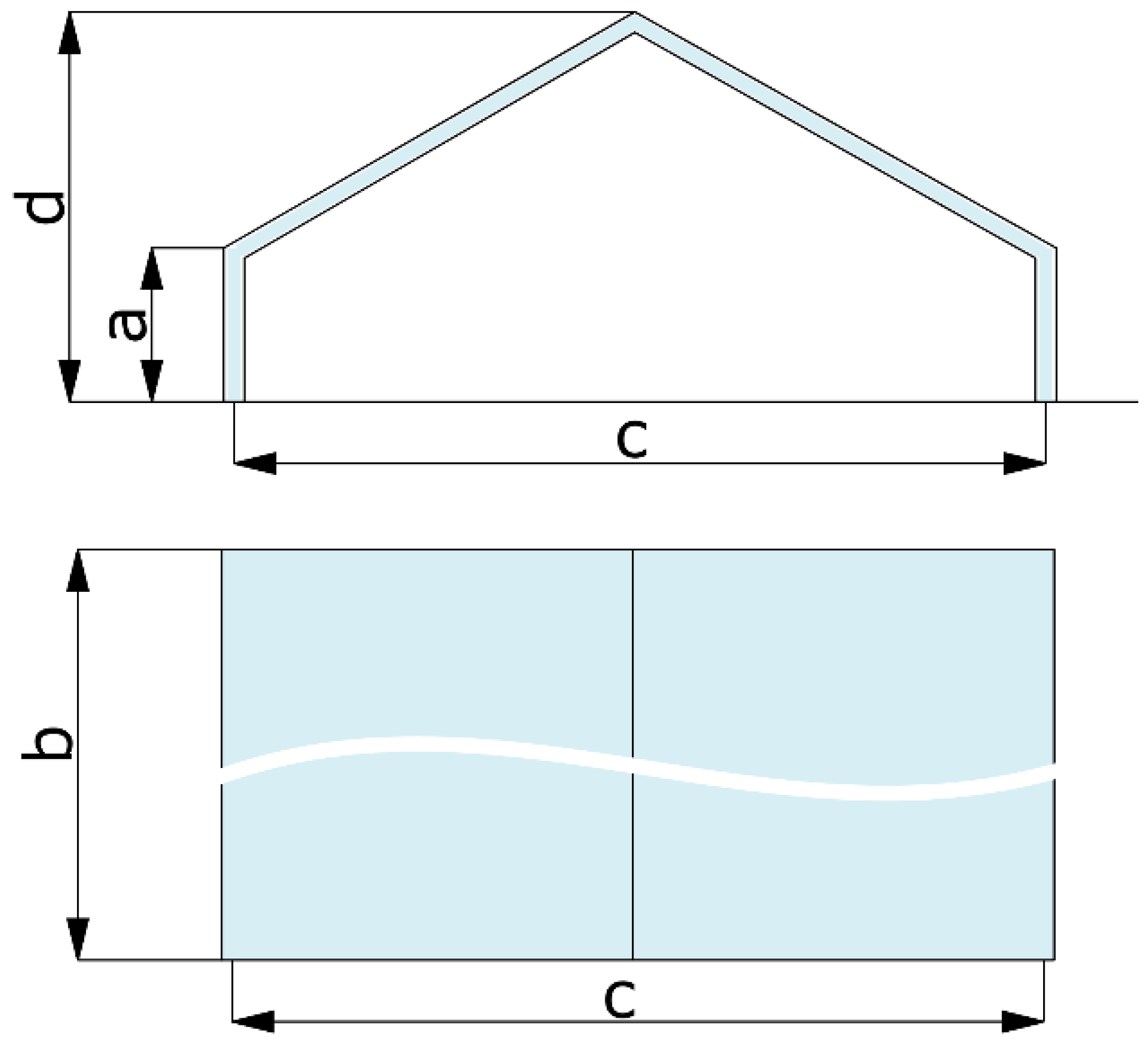
Thermal balance aims to determine the losses and heat gains of each partition in an examined object. For this purpose, calculations of losses by the lateral surface, the upper surface and the ground, as well as the gains from solar radiation that reaches the object during sunny days, known as radiation heat, were conducted. Figure 2 presents the dimensions of the analyzed roof surfaces.

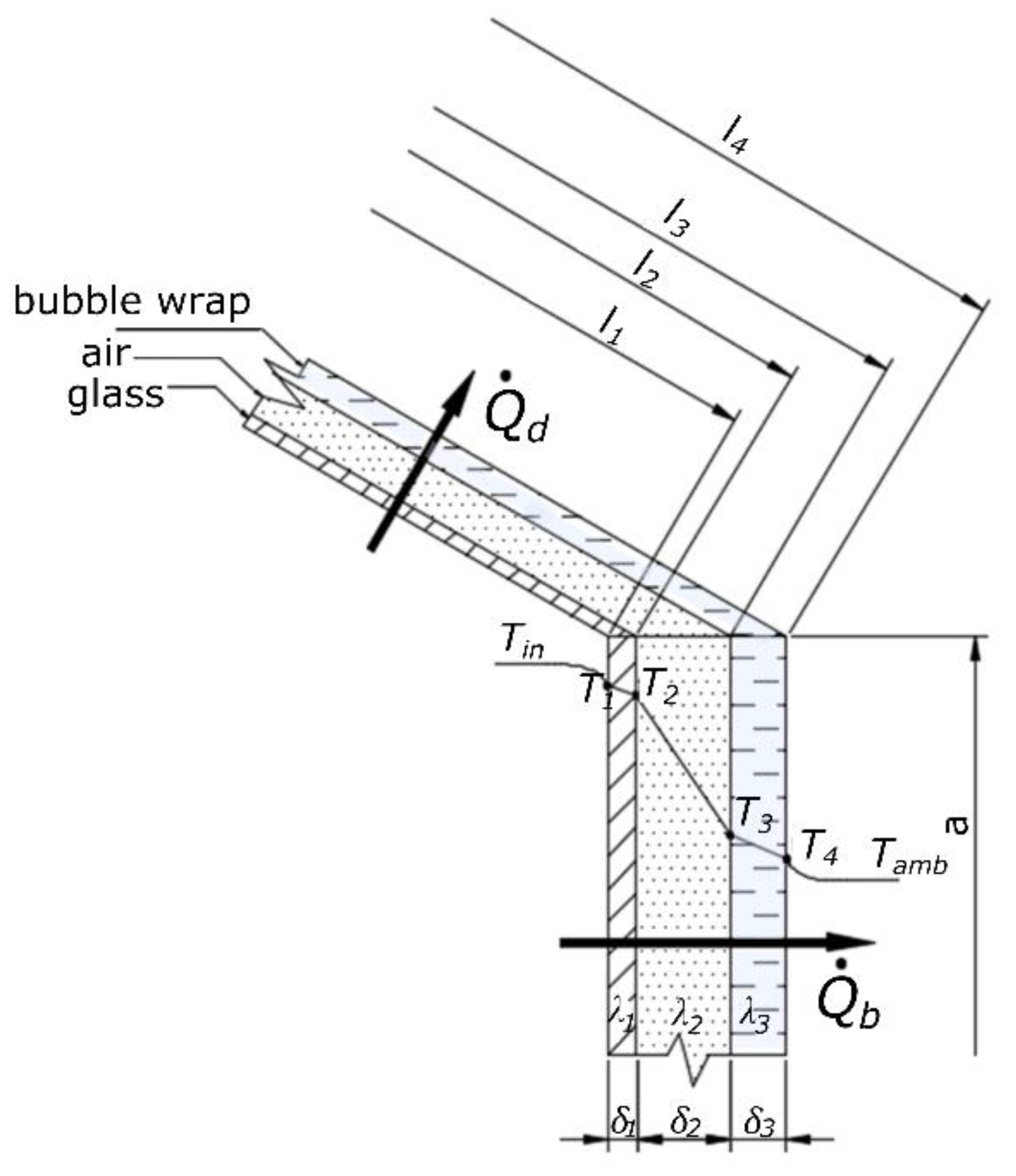
Calculations of the heat gains and losses were made with the assumption that the air between the glass layer and the cell foil, as well as that found inside the greenhouse, is stationary, and therefore there is natural convection. Due to small changes in wind speed in the analyzed period, it was assumed that the average wind speed $w$ outside the greenhouse was equal to 2 m/s. This value corresponds to the averaged meteorological data for the given area.

By knowing the dimensions of the walls, the characteristic linear dimensions should be determined. For the front wall, it is expressed by the formula for the arithmetic mean of the sidewall height a and the height of the greenhouse d (Equation (1)).

$$w_{h,p}=\frac{a+d}{2}$$

(1)

The internal roof slope length $l_1$ was assumed as the characteristic linear dimension of the roof surface (Equation (2)).

$$w_{h,d}=l_1$$

(2)

For the side walls, the height of a side wall $a$ was assumed as the characteristic linear dimension (Equation (3)).

$$w_{h,s}=a$$

(3)

For the ground surface, the diagonal of the surface is assumed as the characteristic linear dimension (Equation (4)), where $c$ is its width and $b$ is its length.

$$w_{h,g}=\sqrt{b^2+c^2}$$

(4)

To characterize the heat exchange process, it was necessary to determine the Reynolds number for the air parameters outside the greenhouse, which was described using Equation (5).

$$Re=\frac{w·w_h}{v_{out}}$$

(5)

The obtained values of the Reynolds number (Table 1) show the turbulent movement of air outside the greenhouse, and also determine the selection of subsequent equations. The equation for the Nusselt number for the outer surface of the greenhouse is described using Equation (6).

$$N{u}_{out}=0.644·R{e}^{0.5}·P{r}^{0.33}$$

(6)

There is a free convection inside the greenhouse, which is why the Nusselt number $N{u}_{in}$ is determined using Equation (7). It depends on the coefficient $C_w$, the Grashof number $G{r}_{in}$, the Prandtl number $P{r}_{in}$ (Table 1) and the coefficient $n_{won}$, the value of which is equal to $n_{in}=1/4$ [28].

$$N{u}_{in}=C_w·{\left(G{r}_{in}·P{r}_{in}\right)}^{n_{in}}$$

(7)

The value of constant $C_w$ in Equation (8) is an indispensable element for determining Nusselt numbers for individual vertical partitions from the inside of an object, and it depends on the Prandtl number $P{r}_{in}$, the value of which is in Table 1.

$$C_w=0.8·{\left[1+{\left(1+\frac{1}{\sqrt{P{r}_{in}}}\right)}^2\right]}^{-\frac{1}{4}}$$

(8)

The compressibility of fluid in Equation (9) is determined for the layer next to a wall. It is a value that depends on the temperature inside an object $T_{in}$ and the temperature of the partition that is directly in contact with the liquid $T_1$. In the analyzed case, this temperature is the temperature of the inner surface of the glass for the front partition and for each of the other partitions.

$$\beta =\frac{1}{\frac{T_{in}+T_1}{2}}$$

(9)

The Grashof number (Equation (10)) depends on: the compressibility of fluid $\beta$ (Equation (9)), the temperature inside a greenhouse $T_{in}$, the characteristic dimensions $w_h$ (Equations (1)–(3)), the acceleration of gravity g, the inner temperature of the glass layer $T_1$, and the kinematic viscosity of the air inside the greenhouse $v_{in}$ (Table 1).

$$G{r}_{in}=\frac{g·\beta ·\left(T_{in}-T_1\right)·w_h{}^3}{v_{in}{}^2}$$

(10)

For a flat partition inclined at an angle of $\phi =30°$, the Nusselt number is calculated from Equation (11).

$$N{u}_{in}=0.56·{\left(G{r}_{in}·P{r}_{in}·cos\phi \right)}^{0.25}$$

(11)

The coefficient of heat transfer from the inside of the greenhouse to the wall for individual partitions depends on the Nusselt number $N{u}_{in}$ (Equations (7) and (11)), the thermal conductivity coefficient ${\lambda }_{in}$ for the liquid in the object (Table 1), and the characteristic dimension of the partition $w_h$ (Equations (1)–(3)). It is expressed using Equation (12).

$$h_{in}=\frac{N{u}_{in}·{\lambda }_{in}}{w_h}$$

(12)

The heat transfer coefficient outside the greenhouse depends on the Nusselt number (Equation (6)), the thermal conductivity coefficient ${\lambda }_{out}$ (Table 1) of the fluid surrounding the object, and the characteristic dimension $w_h$ (Equations (1)–(3)), and is described using Equation (13).

$$h_{out}=\frac{N{u}_{out}·{\lambda }_{out}}{w_h}$$

(13)

The heat transfer coefficient $U$ depends on the thickness of the individual layers of the partition, the conductivity coefficients of the materials from which the partition was constructed (Table 1), and heat transfer coefficients (Equations (12) and (13)), and is described using Equation (14).

$$U={\left(\frac{1}{h_{in}}+\frac{{\delta }_1}{{\lambda }_1}+\frac{{\delta }_2}{{\lambda }_2}+\frac{{\delta }_3}{{\lambda }_3}+\frac{1}{h_{out}}\right)}^{-1}$$

(14)

The heat flux through the partition depends on the heat transfer coefficient $U$ (Equation (14)), the difference between internal temperature $T_{in}$ and external temperature $T_{amb}$, and the heat transfer area $A$ (Table 1), and is described using Equation (15).

$${\dot{Q}}_k=U·\left(T_{in}-T_{amb}\right)·A$$

(15)

The heat flux transmitted between the fluid and the inner wall of the greenhouse (Equation (16)) depends on the coefficient of heat transfer $h_{in}$ (Equation (12)), the temperature difference between the temperature inside an object $T_{in}$ and the temperature of the inner glass layer $T_1$, as well as the surface of heat exchange $A$ (Table 1).

$${\dot{Q}}_{in}=h_{in}·\left(T_{in}-T_1\right)·A$$

(16)

For the roof, the heat transfer coefficient $h_{in}$ (Equation (12)) is increased by 30% in relation to the coefficient calculated for the lateral surface [26]. This is due to the heat flow direction that results from the difference in fluid density, and therefore, for this surface, Equation (16) takes the form of Equation (17).

$${\dot{Q}}_d=1.3·h_{in}·\left(T_{in}-T_1\right)·A_d$$

(17)

Heat of radiation is a result of solar radiation that reaches the interior of an object, and it depends on the intensity of solar radiation $I_c$ that directly falls on a given surface $A_{rad}$, and also the coefficients of transparency of individual partition layers ${\tau }_1,{\tau }_2,{\tau }_3$.

The values of transparency coefficients of the individual layers of a partition of the greenhouse were taken from literature [29]. Their values are given in Table 1.

The volume of the greenhouse $V$ (Equation (18)) is the value that determines the volume of air inside the object. It can be estimated when knowing the geometric dimensions of the greenhouse (Table 1) and the basic formulas for the surfaces of flat figures.

$$V=b·\left(a·c+\frac{c·\left(d-a\right)}{2}\right)$$

(18)

By knowing both the volume of air inside the greenhouse $V$ (Equation (18)) and the air density ${\rho }_{air}=1.23 \mathrm{kg}/{\mathrm{m}}^3$, it is possible to determine the air mass (Equation (19)).

$$m_{air}={\rho }_{air}·V$$

(19)

It was assumed that solar radiation reaches half of the roof surface $A_{rad}$. Therefore, this area is calculated from the length of the greenhouse side $b$ and the outer length of the roof $l_4$ (Table 1).

$$A_{rad}=b·l_4$$

(20)

The heat flux penetrating into the greenhouse due to radiation (Equation (21)) depends on the transparency coefficients of the individual layers of a partition ${\tau }_1,{\tau }_2,{\tau }_3$ (Table 1), the surface of heat exchange (Equation (20)), radiation intensity $I_c$, and the efficiency of the conversion process $\eta$ that defines the amount of radiation energy converted into sensible heat, which takes the value of $\eta =0.7$ [29].

$${\dot{Q}}_{rad}=\eta ·I_c·A_{rad}·{\tau }_1·{\tau }_2·{\tau }_3$$

(21)

The loss of heat to the ground is calculated from heat exchange equation [28] for heat penetration into the ground surface. For this purpose, the series of variables that make this loss are determined. The heat flux depends on the surface of heat exchange $A_g$ and the difference between the ground temperature $T_g$ and the temperature inside the object $T_{in}$, as well as the soil conductivity coefficient ${\lambda }_g$ and the heat transfer coefficient $h_{in,g}$.

The compressibility of fluid (Equation (22)) next to the ground surface depends on both the temperature inside the greenhouse $T_{in}$ and the ground temperature $T_g$.

$${\beta }_g=\frac{1}{\frac{T_{in}+T_g}{2}}$$

(22)

The Grashof number depends on the compressibility of fluid ${\beta }_g$, the difference between the temperature inside the greenhouse $T_{in}$ and the ground temperature $T_g$, kinematic viscosity $v_{in}$ (Table 1) and the characteristic linear dimension $w_{h,g}$ (Equation (4)). It is expressed by Equation (23).

$$G{r}_{in,g}=\frac{g·{\beta }_g·\left(T_{in}-T_g\right)·w_{h,g}{}^3}{v_{in}{}^2}$$

(23)

The Nusselt number inside the greenhouse for the ground surface (Equation (24)) depends on the coefficient $C_w=0.135$ [26], the Grashof number $G{r}_{in,g}$ (Equation (23)), the Prandtl number $P{r}_{in}$ (Table 1) and coefficient $n_{in}$, the value of which is equal to $n_{in}=1/4$ [30].

$$N{u}_{in,g}=C_w·{\left(G{r}_{in,g}·P{r}_{in}\right)}^{n_{in}}$$

(24)

The coefficient of heat transfer to the ground $h_{in,g}$ (Equation (25)) depends on the Nusselt number $N{u}_{in,g}$ (Equation (24)), the air conductivity coefficient ${\lambda }_{in}$ (Table 1) and the characteristic linear dimension of the ground $w_{h,g}$ (Equation (2)).

$$h_{in,g}=\frac{N{u}_{in,g}·{\lambda }_{in}}{w_{h,g}}$$

(25)

The heat flux that penetrates the ground is expressed by Equation (26), where the ground temperature $T_g$ is assumed to be the ambient temperature $T_z$. The flux depends on the surface of heat exchange $A_g$ (Table 1) and the difference between the temperature inside an object $T_{in}$ and the ground temperature $T_g$, as well as the heat transfer coefficient $h_{in,g}$, the ground heat conductivity coefficient ${\lambda }_g$ and the equivalent ground thickness ${\delta }_g$, the value of which is assumed to be 2 m [25].

$${\dot{Q}}_g=\frac{A_g·\left(T_{in}-T_g\right)}{\frac{1}{0.7·h_{in,g}}+\frac{{\delta }_g}{{\lambda }_g}}$$

(26)

The heat flux of ventilation that was caused by greenhouse leaks is related to the specificity of this type of facility and depends on the total area of covers $A_c$ and the resistance to heat transfer that is associated with the air exchange $R_L$, as well as the difference between the temperature inside the greenhouse $T_{in}$ and the temperature outside $T_{amb}$. The total area of the covers $A_c$ (Equation (27)) is the sum of the surfaces of the side walls $A_s$, the front and back walls $A_p$ and also the roof surface $A_d$ (Table 1).

$$A_c=A_s+A_p+A_d=769.93 m^2$$

(27)

The heat flux that is associated with the ventilation of the object ${\dot{Q}}_L$ is expressed by Equation (28), where the value of the thermal resistance is equal to $R_L=0.5 \frac{m^{2}K}{W}$ [25].

$${\dot{Q}}_L=\frac{A_c}{R_L}·\left(T_{in}-T_{out}\right)$$

(28)

The computational algorithm that allows the above heat exchange equations to be solved was prepared in Mathcad 15 software. It enabled the heat flux that penetrates the individual partitions, as well as the temperature of the inner wall $T_1$ and the final temperature inside the object $T_k$ to be determined. The above-mentioned activities allowed the balance in Equation (29) to be written, which in turn enabled the temperature in the greenhouse $T_{in}$ after the specific time step $t$ to be determined.

$$m_{air}·c_{p,air}·\left(T_{in}-T_{out}\right)=\left[{\dot{Q}}_{rad}-\left({\dot{Q}}_d+{\dot{Q}}_s+{\dot{Q}}_p+{\dot{Q}}_g+{\dot{Q}}_L\right)\right]·t$$

(29)

3.1. Calculation of the Temperature Inside the Greenhouse

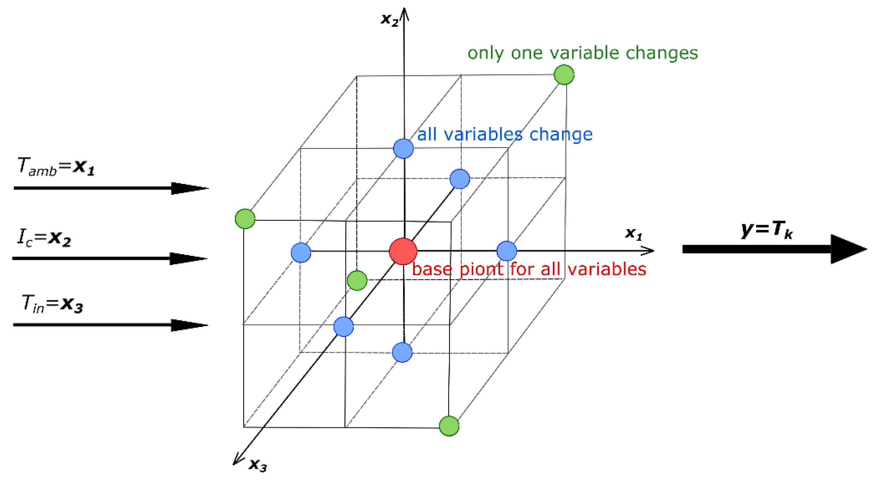
To determine the final temperature inside the greenhouse, techniques of planning an experiment were used. A three-level plan for three input factors on three levels of variation, called the Hartley plan [31], was chosen for the analysis. The use of it enabled the dependence between the final temperature inside the greenhouse $t_k$ and the three following input factors to be determined (Figure 3):

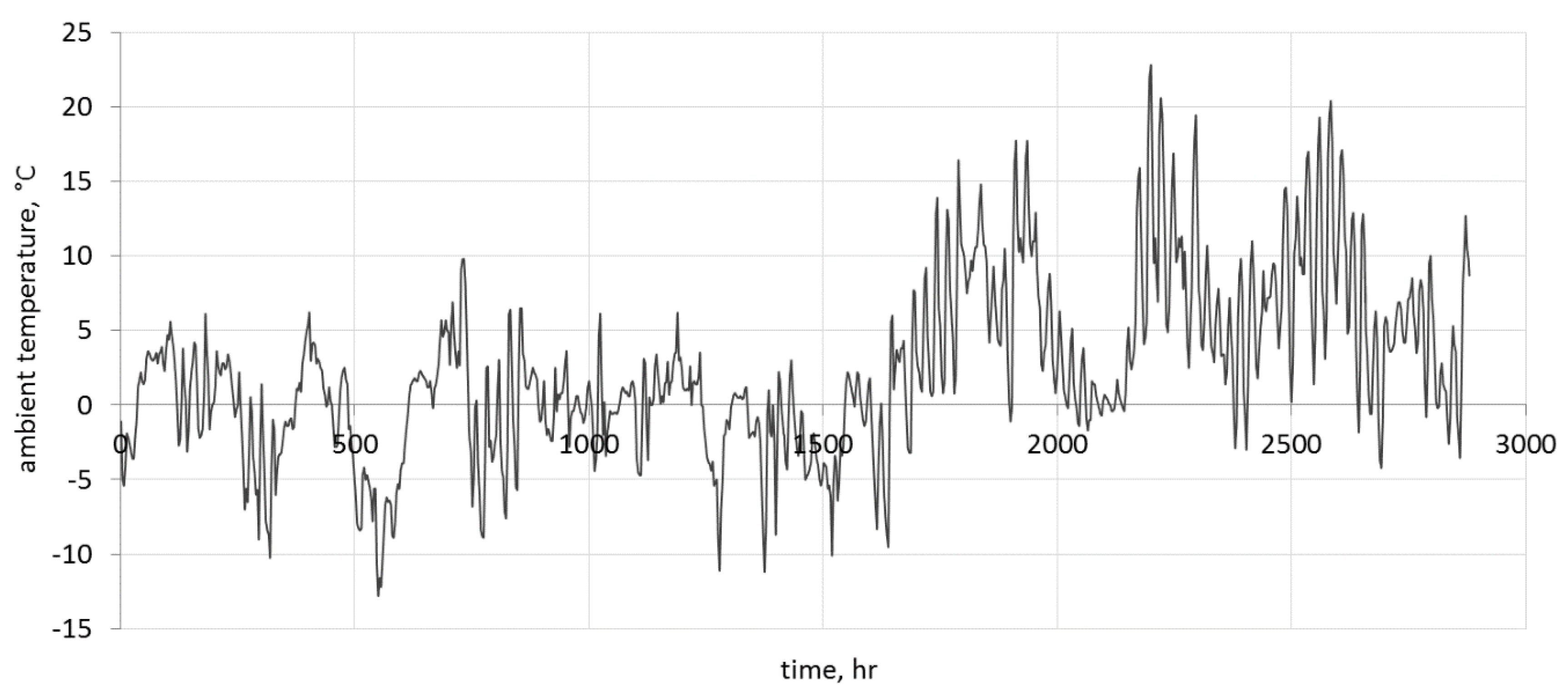
• $x_1$—ambient temperature $T_{amb}$ that varies within the range from −12.8 to 22.8 °C;
• $x_2$—intensity of solar radiation $I_c$ that covers the range from 0 to 447.3 W/m²; and
• $x_3$—temperature inside the greenhouse $T_{in}$, which can take values from −12.8 to 50 °C.

The Hartley Plan matrix for the three input factors, which is built on the hypercube, is shown in

Table 2. Characteristic parameters of the greenhouse.

No.	${\mathit{x}}_{\mathbf{1}}$	${\mathit{x}}_{\mathbf{2}}$	${\mathit{x}}_{\mathbf{3}}$
1	+	+	+
2	+	−	−
3	−	+	−
4	−	−	+
5	+	0	0
6	−	0	0
7	0	+	0
8	0	−	0
9	0	0	+
10	0	0	−
11	0	0	0

In the statistical plan, the + sign indicates the maximum value of the input variable, 0 the average value and the − sign the minimal value.

.

The implementation of Hartley’s plan allows a mathematical model that describes the temperature changes inside the greenhouse with regards to the input factors, which is expressed by means of the second degree polynomial (Equation (30)), to be determined.

$$y=T_k=a_1+a_2{T}_{amb}+a_3{T}_{amb}{}^2+a_4{I}_c+a_5{I}_c{}^2+a_6{T}_{in}+a_7{T}_{in}{}^2+a_8{T}_{amb}{I}_c+a_9{T}_{amb}{T}_{in}+a_{10}{I}_c{T}_{in}+a_{11}{T}_{amb}{I}_c{T}_{in},$$

(30)

Determination of the linear-quadratic equation starts with the calculation of the central values (Equations (31)–(33)), thus the determination of the input variables that assumes the 0 level.

$$x_{10}=\frac{T_{out,max}+T_{out,min}}{2}=5 °\mathrm{C}$$

(31)

$$x_{20}=\frac{I_{c,max}+I_{c,min}}{2}=223.65 \mathrm{W}/{\mathrm{m}}^2$$

(32)

$$x_{30}=\frac{T_{in,max}+T_{in,min}}{2}=31.4 °\mathrm{C}$$

(33)

Table 3. Values of input variables.

	−1	0	1
${\mathit{T}}_{\mathit{a}\mathit{m}\mathit{b}}, °\mathrm{C}$	−12.8	5	22.8
${\mathit{I}}_{\mathit{c}}, W/m^2$	0	223.65	447.3
${\mathit{T}}_{\mathit{i}\mathit{n}}, °\mathrm{C}$	−12.8	31.4	50

presents the values of individual variables that assume the three levels of +1, 0 and −1 successively.

The values of individual linear-quadratic equation coefficients (Equation (30)) were determined using matrix markers, and their values are presented in

Table 4. Values of regression coefficients for the equation, and also simulation results.

No.	Regression Coefficient, -	Final Temperature, °C
1	1.799320052209	35.6
2	1.073490373906	22.8
3	0.000315616715	−3.3
4	0.030137100946	−5.4
5	−0.000001699343	29.6
6	0.134666158924	−5.8
7	−0.000157275535	16.7
8	0.000125349535	6.7
9	−0.005856511074	12.5
10	−0.000298081806	9.7
11	0.000010479794	11.8

. Table 4 also shows the simulation results for individual combinations of input variables according to the Hartley matrix.

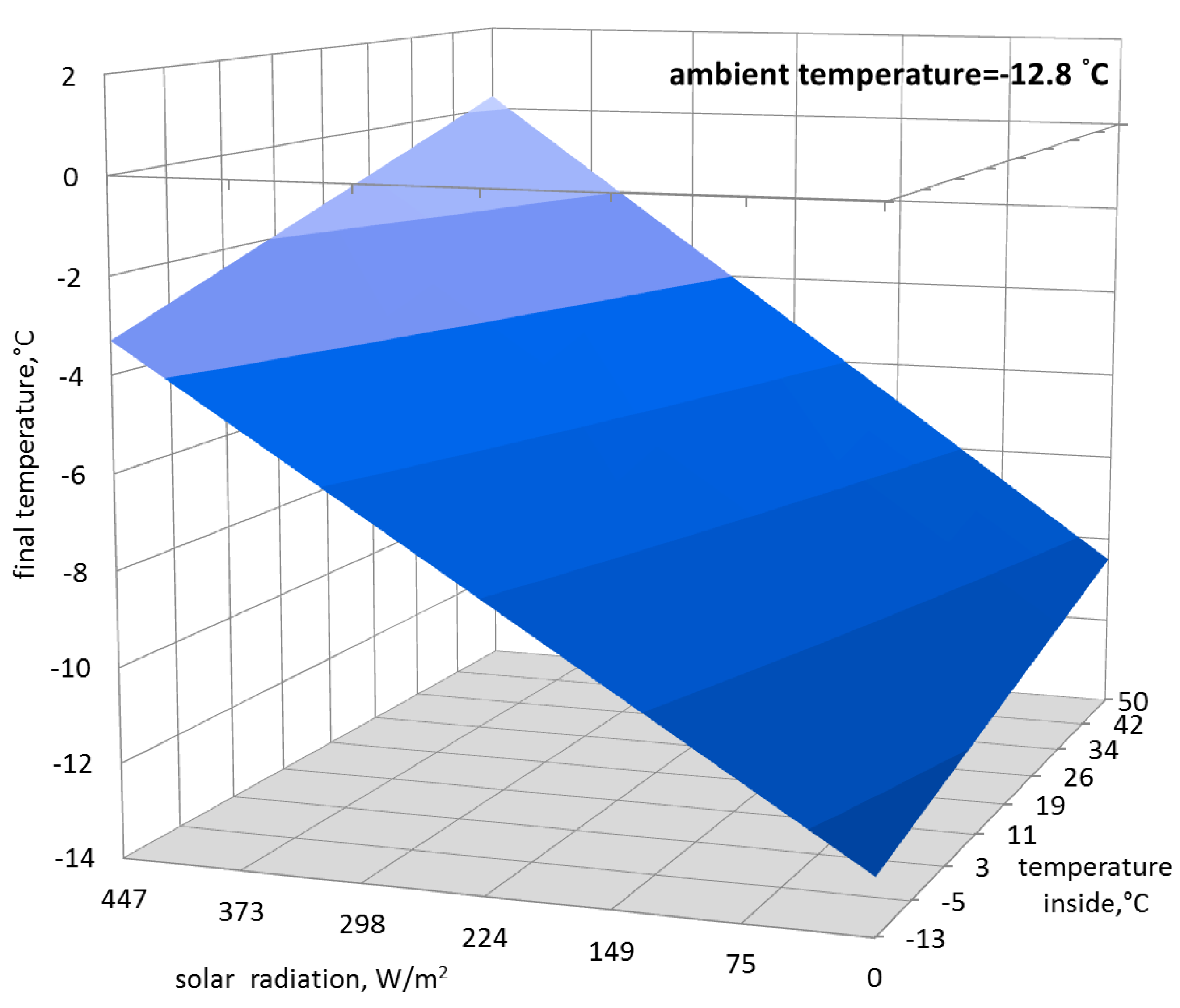
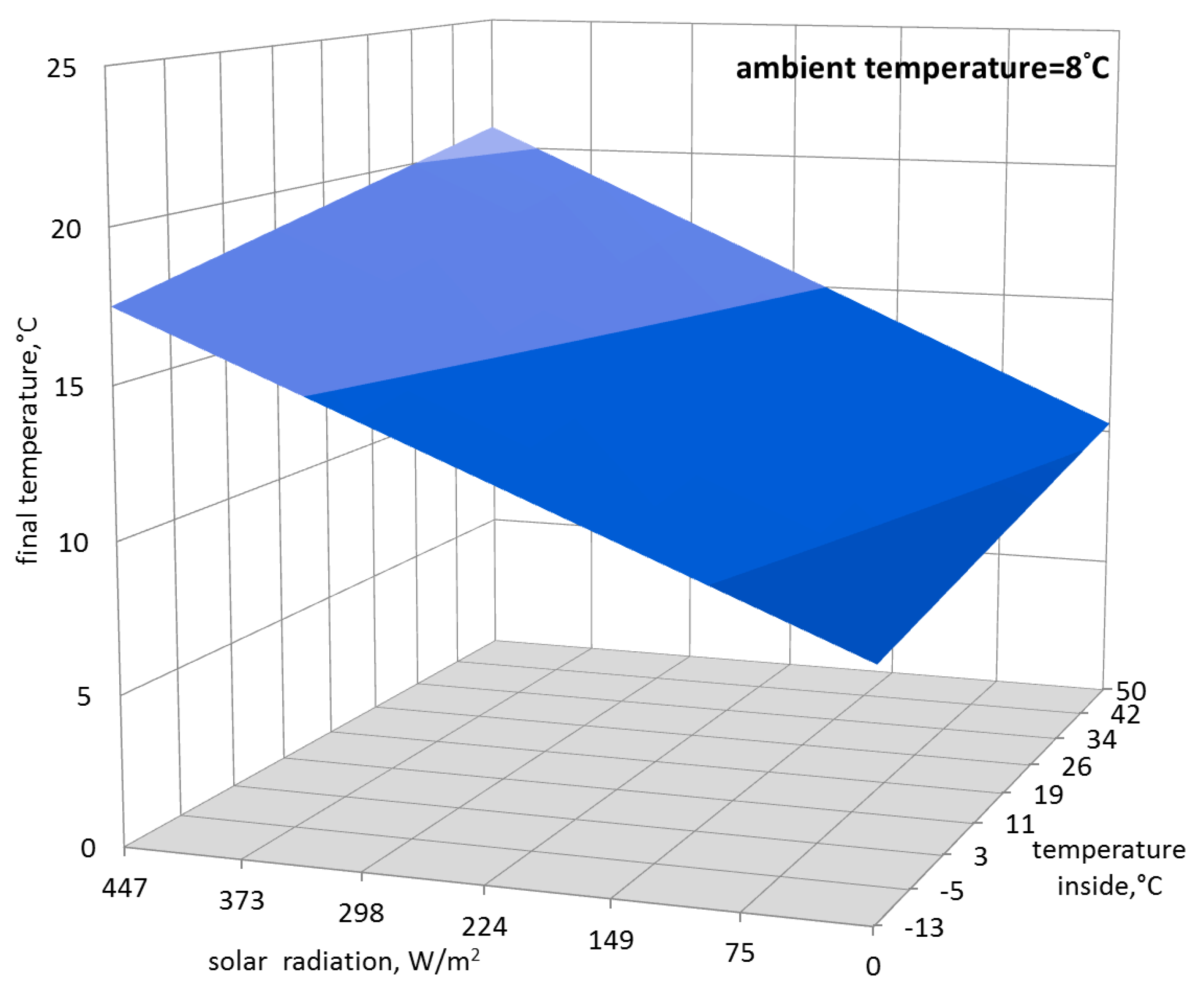
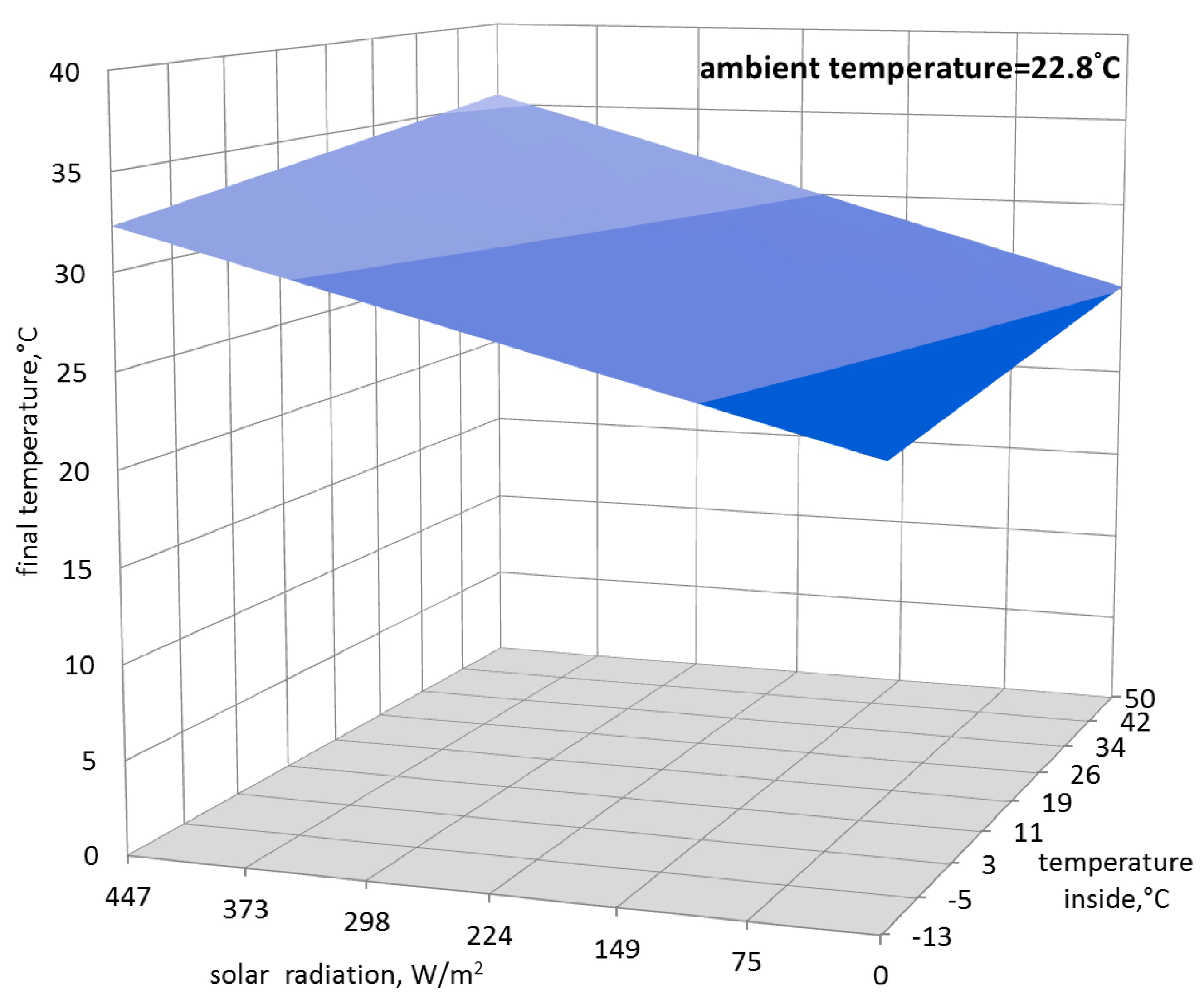
Based on the obtained function, it was possible to determine the final temperature inside the greenhouse with regards to the three above-mentioned input parameters, which is shown in Figure 4, Figure 5 and Figure 6.

The obtained equation for the temperature inside the greenhouse was used to prepare the heat demand for the analyzed heating period.

3.2. The Greenhouse’s Heat Demand

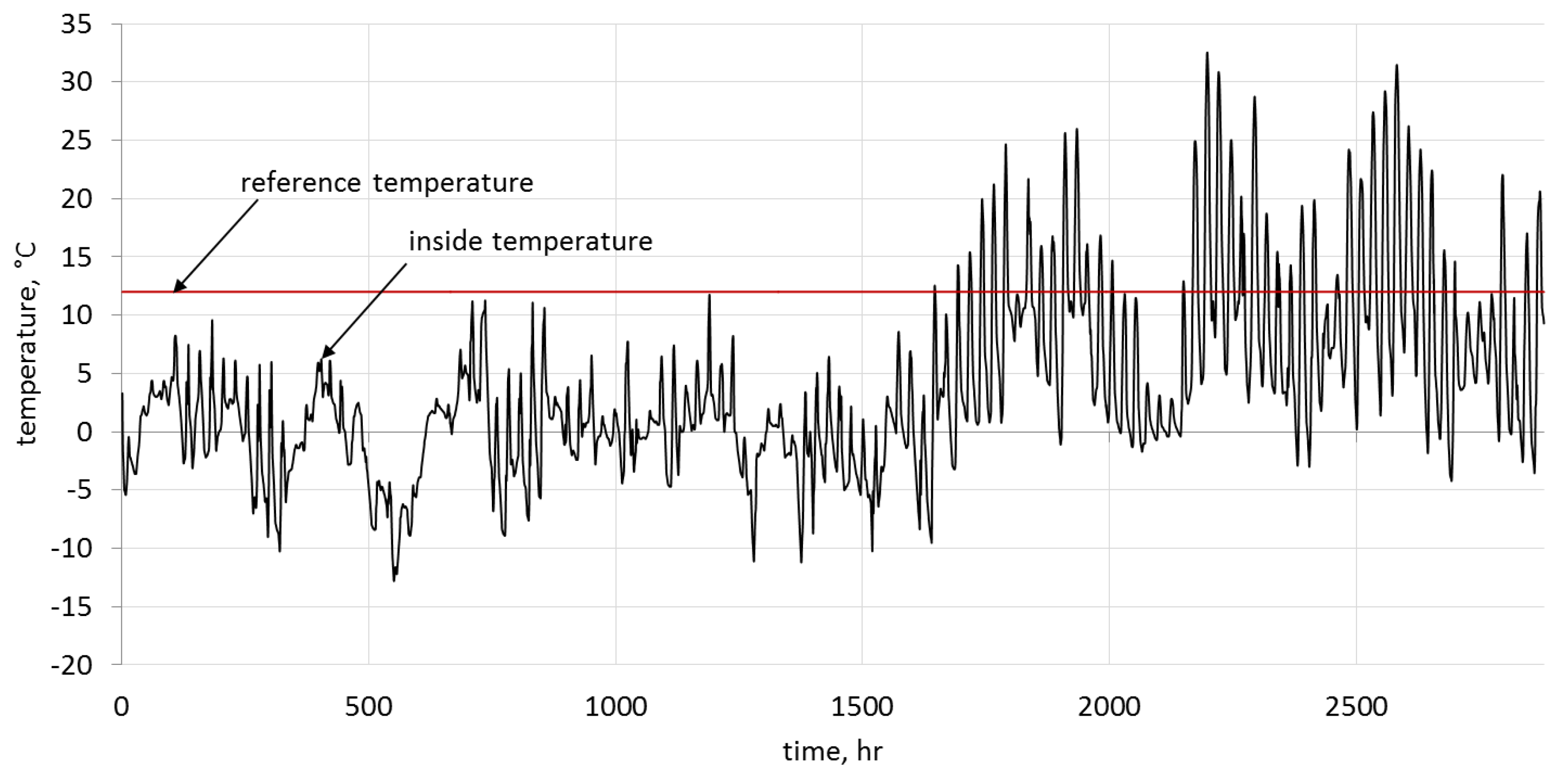
To determine heat demands, statistical data published by the Ministry of Investment and Development of the Republic of Poland [32] were used for the energy calculations of buildings for the given location of the greenhouse. Figure 7 shows the change in the temperature inside the object during the day from the beginning of January until the end of April. In the analyzed period, the temperature inside the greenhouse is lower than the reference temperature of 12 °C. This proves that a heating system needs to be used during this time.

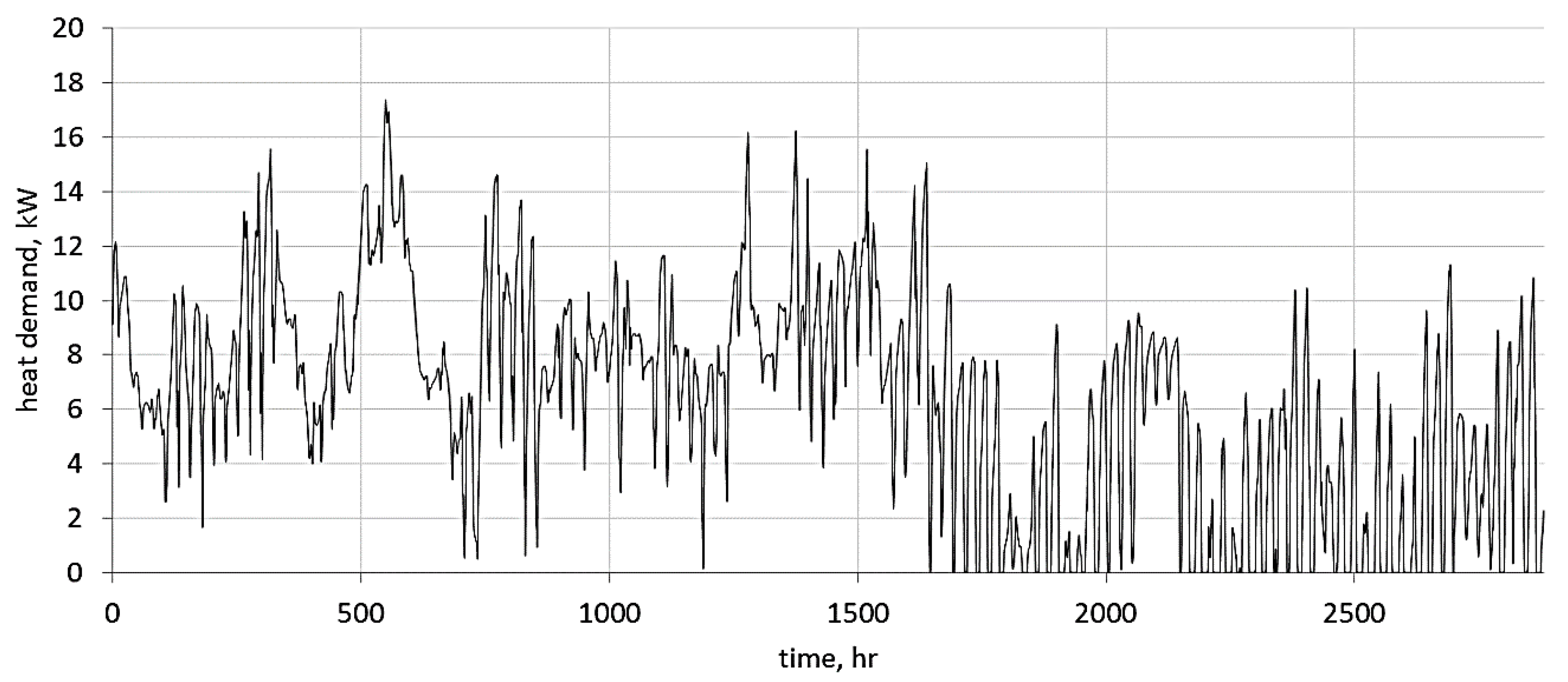
Figure 8 presents the characteristics of the greenhouse’s heat demand, which was created on the basis of the thermal balance equations of the greenhouse.

The obtained characteristics determine the minimum power of the heating system and are the basis for determining the operating costs.

4. Selection of the Heating System

Based on the obtained characteristics of the heat demand for the greenhouse, it is possible to select a heat pump with an appropriate power. The heat power of the heat pump was determined with regards to the maximum heat demand in the given facility. For this purpose, it was assumed that there is no solar radiation $I_c=0 \raisebox{1ex}{$W$}\!\left/ \!\raisebox{-1ex}{${\mathrm{m}}^2$}\right.$, and the ambient temperature has the lowest value for the considered period of $T_{amb}=-12.8 °\mathrm{C}$. The obtained value of the maximum heat flux was equal to ${\dot{Q}}_h$ = 17,360 W. The power of the heat pump should not be less than the value of the calculated heat demand of the greenhouse. However, too high a power of a heat pump in relation to the requirements of the heated object generates higher costs and may cause impulse pump operation. This leads to a reduction of the device’s durability. Two types of heat pumps were analyzed in order to determine the validity of their application for the climatic conditions of Poland.

4.1. Simulation of the Operation of a Ground Source Heat Pump

A glycol/water heat pump with a power of 21.5 kW for S0/W35 was selected from those available on the market, for which the parameters are listed in

Table 5. Selected parameters of the selected heat pump.

Parameter	Unit	Value
Heating power at S0/W35	kW	21.5
Performance factor at S0/W35	-	4.66
Total mass	kg	345
Sound pressure level	dB(A)	54.6
Refrigerant (R410A)	kg	6.0
Dimensions (width × length × height)	mm	1242 × 860 × 1154
Scope of work (external temp.)	°C	−5–20

. The COP in the function of ground temperature was read from the catalog sheet of the selected heat pump (Figure 9).

The garden complex on which the analyzed greenhouse is located is a large object, and it was therefore decided to choose a horizontal heat exchanger as the lower heat source. The selected heating device is to be used in a monovalent system of work, covering one hundred percent of the heat demand. To determine the amount of energy that is needed for the heat pump to operate, it was necessary to determine the COP throughout the entire analyzed period, which is dependent on the temperature of the ground and the temperature in the greenhouse. For this purpose, the annual temperature distribution in the ground was read from AWADUKT Thermo software, which is available on the manufacturer’s website (REHAU) of ground heat exchangers. The temperature changes in the analyzed months for the ground at a depth of 1.8 m, which is treated as dry quartz sand, is shown in Figure 10.

The temperature of the heat pump’s upper heat source is equal to 35 °C (the lowest possible setting). By knowing that the temperature of the lower heat source changes, as shown in Figure 10, it was possible to determine the COP for the analyzed period of time (Figure 11).

Electric energy consumption is calculated by knowing the energy demands of a given facility (Figure 8), as well as the value of the COP (Figure 11). It is possible to determine the electricity consumption N that was used by the heat pump in every hour of its operation using Equation (34).

$$N=\frac{{\dot{Q}}_h}{COP}$$

(34)

Figure 12 shows the consumption of electricity $N$ over time for the evaluated greenhouse.

4.2. Simulation of the Operation of an Air Source Heat Pump

An air source heat pump is an alternative heating system that can be used for greenhouse heating. The algorithm for determining the energy demands of an air source heat pump is the same as for the ground source heat pump. However, the lower heat source changes, which is much more unstable. Changes in air temperature for the considered location are presented in Figure 13. These are hourly values, which are available on the website of the Ministry of Investment and Development of the Republic of Poland [32].

For the lowest temperature, which is equal to −12.8 °C, the thermal demands of the greenhouse amounted to 17.36 kW (Figure 8). Therefore, the heat power of the air source heat pump should be selected for such assumptions. Figure 14 presents the characteristics of the thermal power of the selected heat pump, the nominal thermal power of which is equal to 23 kW.

Based on the COP characteristics in a function of temperature (Figure 14), the COP was determined for the entire analyzed working time (Figure 15). When comparing Figure 11 and Figure 15, it is possible to notice a greater unevenness in the parameters of the air source heat pump, which is a result of larger temperature changes in the lower heat source.

To determine the energy expenditure on the operation of the air source heat pump, the heat demands (Figure 8) and the COP (Figure 14) should be known.

Using Equation (34), it was possible to determine the energy demands (Figure 16) for a given time step (1 h).

5. Economic Analysis

The cost of a heating installation includes fixed and variable costs. For the analyzed heating system, the heat pump is a fixed cost. The price of the chosen ground source heat pump, according to the company’s price list, is equal to €10,049 gross. The price of executing a horizontal collector is around €4285. The cost of the entire investment $K_{I,hp1}$ of €14,334 is obtained by adding the cost of purchasing a ground source heat pump and installing a ground collector. Calculated per unit of the greenhouse area that amounts to 419.92 m², it is equal to €34/m². The cost of an air source heat pump is equal to €4952 gross, and when it is calculated per unit of the greenhouse area, it is equal to €12/m². The cost of producing a boiler room equipped with a coal-fired boiler with an 18 kW feeder is approximately €1904.5 gross. The total cost of assembly is about €1190, and therefore the total investment cost $K_{I,b}$ is estimated to be €3094.5, which, when calculated per unit of the greenhouse area, is equal to €7.4/m².

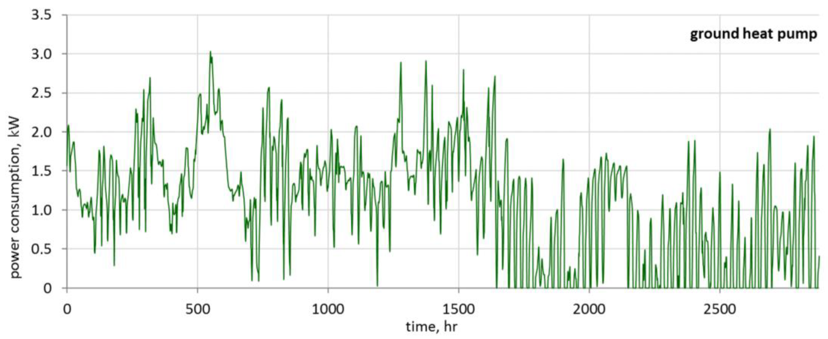
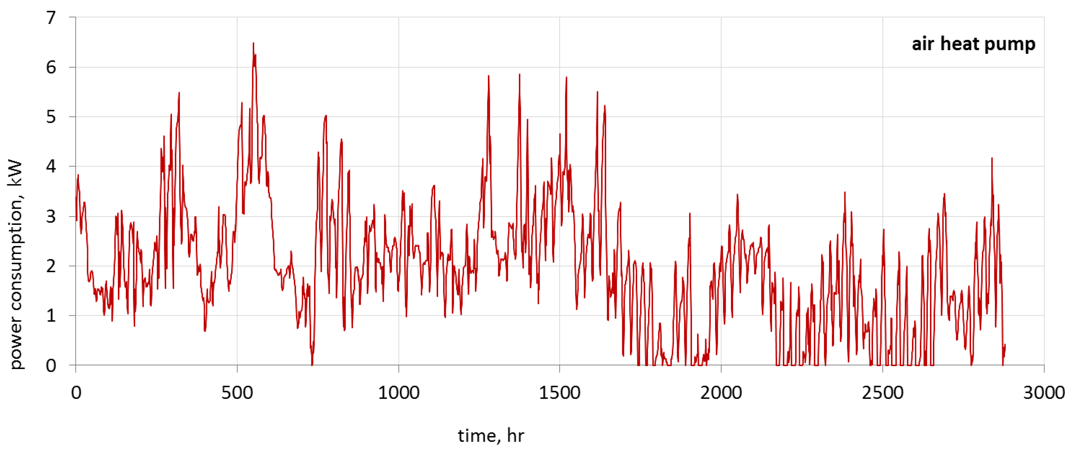
The cost of running a ground source heat pump is calculated on the basis of the characteristics of the consumed electricity (Figure 12). Assuming that 1 kWh costs €0.12, then the cost for the entire heating period $K_{E,hp1}$ is equal to €385.60/year. Using the characteristics presented in Figure 16, the cost of the air source heat pump $K_{E,hp2}$ is equal to €678.64/year.

To calculate the simple payback time of the investment, the costs of the heat pumps’ operation were compared to the costs incurred when heating the boiler with fine coal. Fuel consumption for heating the greenhouse with the existing 25 kW fine coal boiler for the designated heat demands is determined using Equation (35).

$$B=\frac{{\dot{Q}}_h·t}{{\eta }_k·Q_w^r}$$

(35)

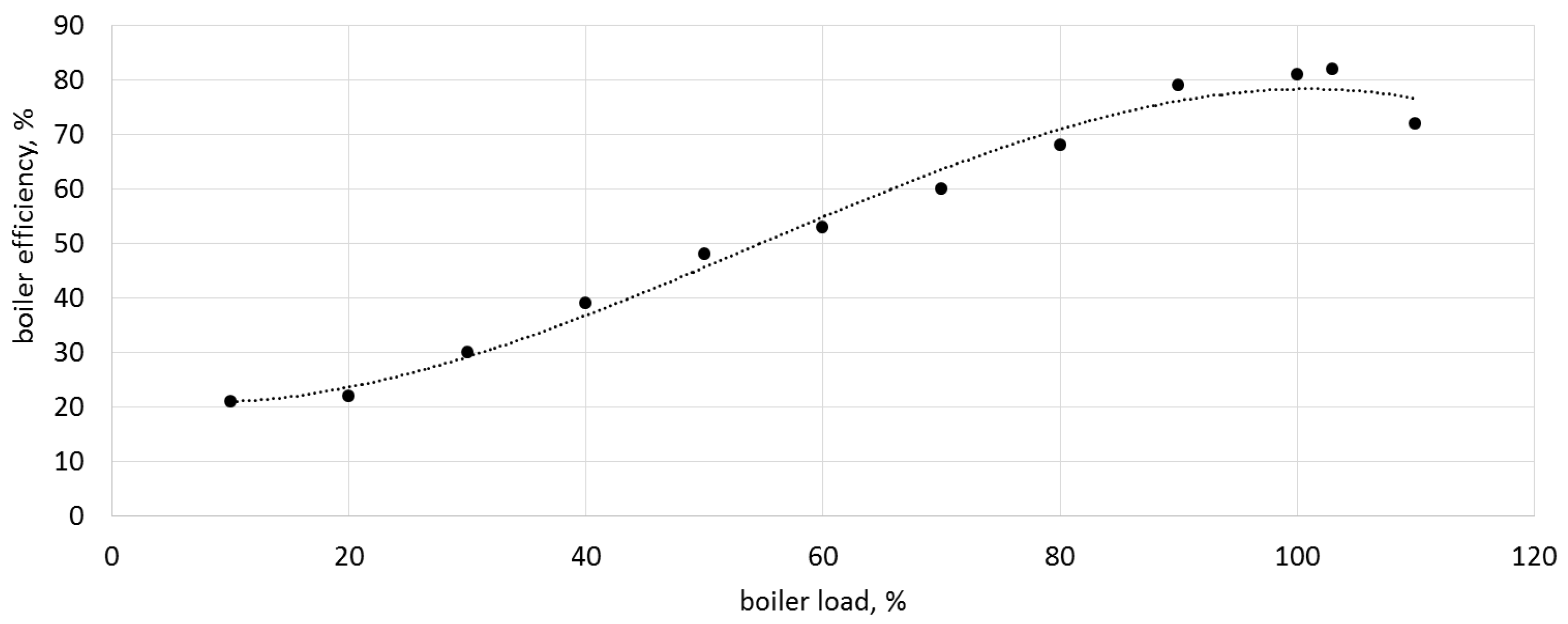
The calorific value of fine coal is assumed to be 18–26 MJ/kg, and therefore the following value is assumed for the calculations: $Q_w^r=20 \mathrm{MJ}/\mathrm{kg}$. It corresponds to the most common value of coal in this region. The efficiency of the boiler ${\eta }_b$ strictly depends on its load. Therefore, based on the boiler efficiency characteristics, a function describing this dependence was determined, which allows the amount of burned fuel (Figure 17) to be more accurately analyzed.

The consumption of coal dust in the analyzed period of four months amounted to 7670 kg, therefore, considering the average price of coal dust of €135.71 per tonne, it is estimated that the cost of heating the greenhouse was equal to $K_{E,b}$ €1040.90/year. This value is consistent with the costs borne by the owners of the greenhouse. The obtained profit Z (Equation (36)) is the amount of money that the facility user would have to bear for its heating in the case of a lack of installation that uses a heat pump. It is the difference between the costs incurred for the coal boiler $K_{E,b}$ and the operating costs related to heating the greenhouse with the heat pump $K_{E,hpi}$.

$$Z=K_{E,b}-K_{E.hpi}$$

(36)

The simple payback time for the investment $L$ (Equation (37)) is the quotient of investment costs $K_I$, which are the difference between the cost of a boiler room using the heat pump $K_{I,hpi}$ and that equipped with a boiler with a feeder $K_{I,b}$, and profits $Z$:

$$L=\frac{K_{I,hpi}-K_{I,b}}{Z}$$

(37)

A simple payback time for a ground source heat pump for the analyzed greenhouse facility is 18 years. The lifetime of the heat pump compressor is estimated at around 90,000 operating hours, and in the analyzed facility the operation time of the pump is about 2688 h. Considering the average annual time of 2700 h of using the device, the heat pump should theoretically work without failure for about 33 years. The simple payback time for an air source heat pump is 5.5 years. The working time is the same as for a ground source heat pump, and therefore trouble-free working time should also be around 33 years.

6. Emission of Pollution

To estimate the impact of the planned change of the heating system on the environment, calculations of the volume of the emission of pollutants generated by the previous heat source were performed. The volume of emission depends on the type of fuel, its consumption, and parameters such as: calorific value, ash content and also sulfur content [33]. The calculations were made according to Equation (38) [33] for a boiler with a fixed grate, natural draft and thermal power of the boiler of ≤0.5 MW.

$$E=B·W$$

(38)

The parameters of the analyzed solid fuel boiler are summarized in

Table 6. Parameters of the coal boiler so far used.

Fuel	Coal Dust
Fuel consumption	7670 kg
Boiler	18 kW
Sulfur content in hard coal	0.83% [34]
Ash content A’	22.4% [34]

. The results of calculations are presented in

Table 7. Volume of emission of pollutants when using conventional fuel.

Type of Pollution	Amount, g/Mg	Volume of Emission E, kg
		1 Season	5.5 Seasons	18 Seasons
SOx	13,280	101.8	560.2	1840.6
NOx	2200	16.8	92.8	304.9
CO	45,000	345	1898	6237
CO2	1,850,000	14,189	78,042	256,404
TSP	22,400	171.8	944.9	3104.6
benzo (a) pyrene	14	0.107	0.590	1.940

and graphically illustrated in Figure 18 for the payback time of the investment with regards to two heat pumps.

Figure 18 contains information on the amount of emissions of the individual exhaust components (calculation data) from combustion in the existing coal boiler (blue color). The emission values after 5.5 years have been shown in red, because this is the payback time for an air source heat pump. The green color indicates emissions from the boiler for 18 years, because this is the payback time of the ground source heat pump. Since heat pumps are considered to be zero emission (zero “low emission”), it has been called “avoided emissions”.

The demonstrated reductions in pollutant emissions may be crucial when applying for investment subsidies, and this may additionally shorten the payback time of this investment. Moreover, it is an important environmental aspect that has recently begun to play an increasingly important role.

7. Summary and Conclusions

The analysis presented in the article concerned the heating of a greenhouse facility in Polish climatic conditions. The thermal balance of the greenhouse included all inflows of heat from the environment resulting mainly from solar radiation, as well as losses due to heat transfer through the partitions, and also those resulting from the natural ventilation of the greenhouse, which in turn depends on the difference between the interior temperature and the ambient temperature.

The created balance was used to perform a simulation according to the specific assumptions of the Hartley plan. This allowed temperature changes in the facility, assuming a time step of 1 h for the four analyzed months, to be described in detail.

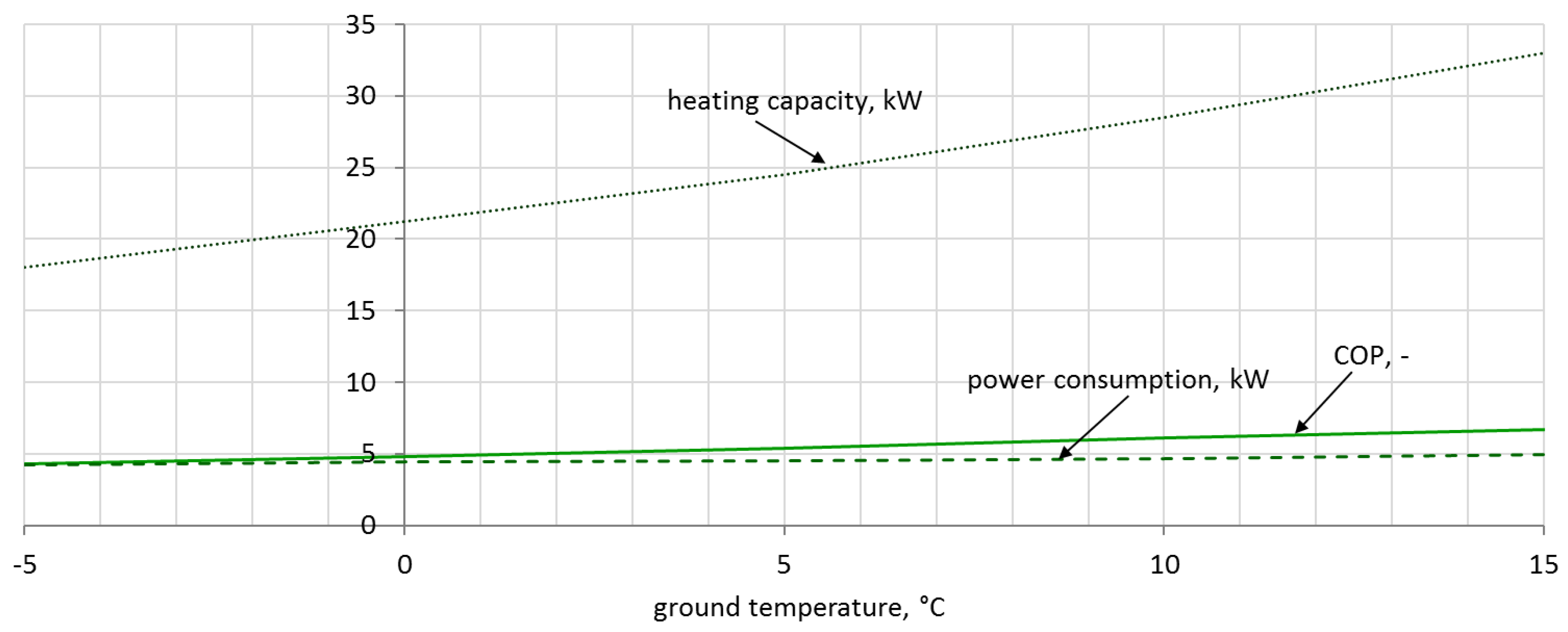
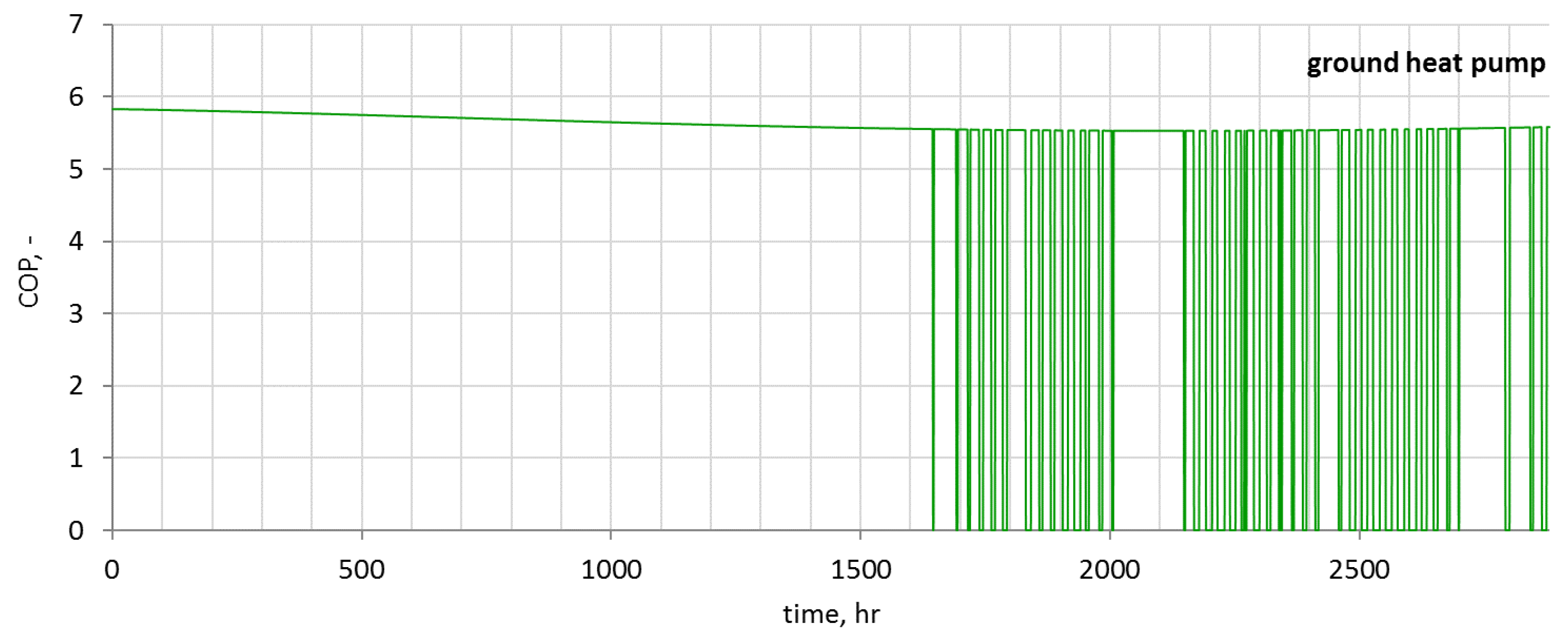
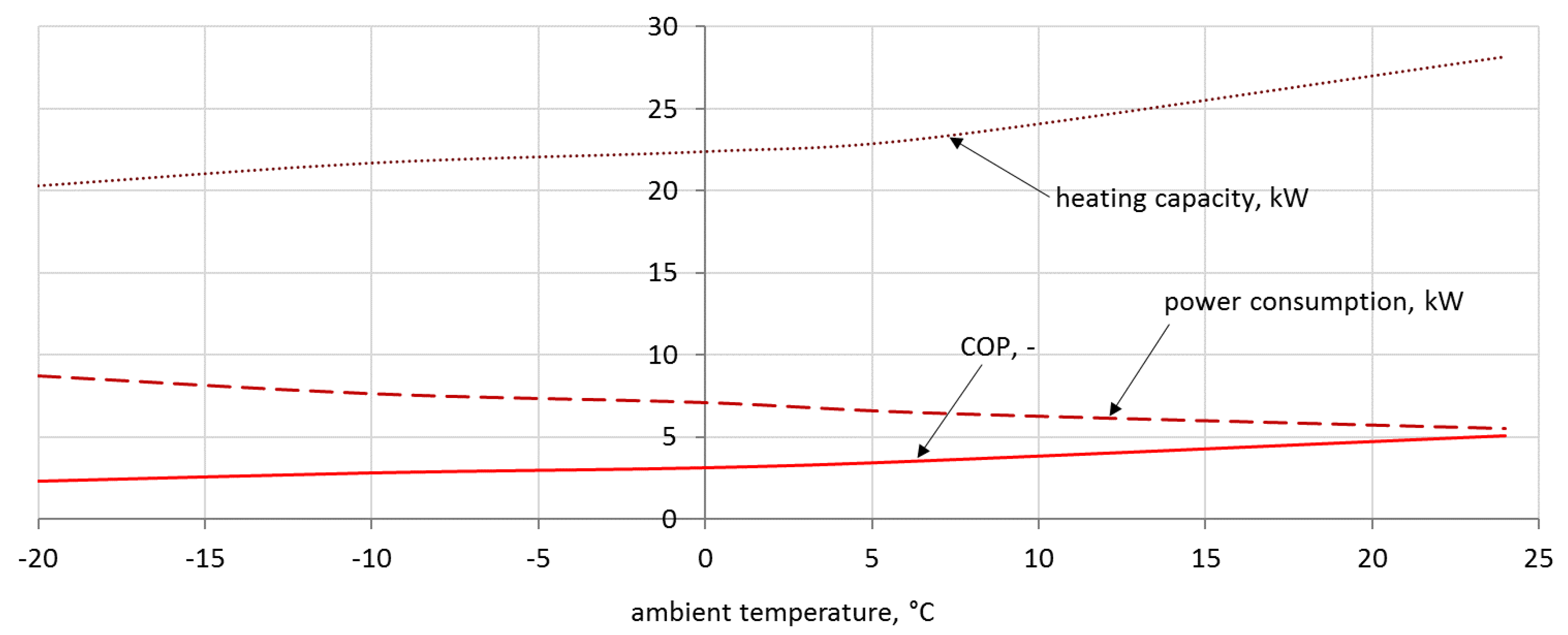
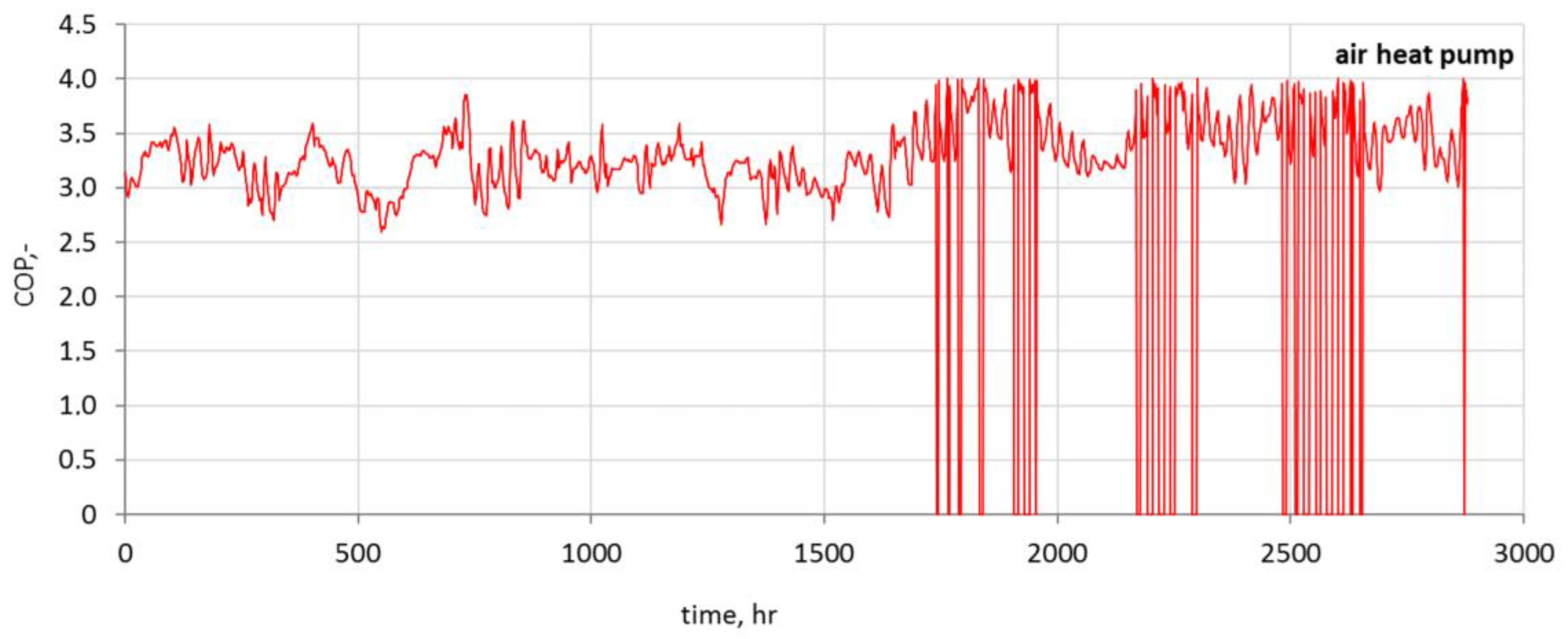
Due to the legal regulations regarding environmental protection, and also the general interest in the use of heat pumps, it was decided to use and analyze ground and air source heat pumps in the greenhouse. The rated power of the selected glycol–water ground source heat pump was equal to 21.5 kW. The analysis showed that the ground source heat pump will work with a COP within the range of 5.53–5.83. For a selected 23 kW air source heat pump, the COP varied 2.59–4.00. Significantly higher changes in ambient temperature, when compared to the ground temperature, resulted in higher energy demands, and therefore in higher operating costs. For the air source heat pump, it amounted to €678.64/year, and for the ground source heat pump it amounted to only €385.60/year.

To estimate the profitability of using a certain heating system, it was necessary to perform economic analysis and calculate the simple payback time of the investment. When comparing the cost of operating a heating system that uses a ground source heat pump with an existing heating system that uses a coal-fired boiler, annual profits reached 62%. The calculation of the simple payback time also included the investment cost, which is more than 3.5 times higher for the ground source heat pump. Therefore, such an investment will pay back after about 18 years. Annual savings from the use of the air source heat pump are smaller and amounted to 32%. However, a much lower investment cost means that the payback time of such an investment is only 5.5 years.

Taking into account all the advantages and disadvantages of a heating system based on a heat pump, and the analysis of the system’s operation, it can be considered as a competitive method of heating greenhouse facilities when compared to traditional coal boilers with regards to the economy and especially with regards to environmental protection.

The air source heat pump has the unstable temperature of the lower heat source. However, this temperature in the analyzed period of time is so high that the device is profitable. The shorter payback time for the air source heat pump means that it should be more often chosen as a greenhouse heating system in Poland’s climatic conditions.