Investigation of Low-Frequency Data Significance in Electric Vehicle Drivetrain Durability Development

Abstract

The digitalization of the automotive industry presents significant potential for technical advantages, such as the online collection of customer driving data. These data can be used for customer-oriented development to improve the durability of components or systems. However, due to current limitations in data transfer, the sampling frequency is typically lower than that of classic dataloggers. This paper examines the importance of low-frequency data in the development of drivetrain durability and investigates the extent to which these data can be utilized for a drivetrain durability analysis. Real driving data were utilized as a database to demonstrate the impact of downsampling on data significance, with the deviation in damage serving as the criteria. The findings suggest that low-frequency data, when available in sufficient quantities, can provide valuable information for predicting durability in rollover and time at level classification. The deviation in the damage prediction is less than 2% for distances exceeding 5000 km. However, low-frequency data are not suitable for rainflow analysis. Finally, the database size was adjusted to assess the statistical stability of the durability prediction. A larger dataset typically reduces variance. The paper presents evidence for the quality and usability of cloud data in drivetrain durability design. Cloud data from a significant number of customer vehicles can be used for certain analyses of representative customer load collectives, which can reduce development time and costs.

1. Introduction

Battery electric vehicles (BEVs) are becoming increasingly popular worldwide, especially in Europe, the USA, and China. The majority of mainstream BEVs on the market use a drivetrain with one electric machine (EM) and a single-speed gearbox, which is suitable for most applications. Recent BEV development has focused on battery and energy management strategies [1,2]. The development of drivetrain durability faces new challenges due to the increased number of electrical components and complexity in the powertrain. Studies have been conducted on the durability of traction batteries [3,4], EM [5], and the electric system [6]. The mechanical components also face more challenging working conditions due to the properties of the EM, such as high-frequency current, as discussed in [7], a wider speed range, and recuperation. During the design process, it is important to take into account that the recuperation with negative torque can result in an additional load on torque transfer components, such as gears.

Insufficient customer data can limit knowledge of actual BEV usage and the loads that customers place on drivetrain systems and components. Durability measurement campaigns are typically conducted with a limited number of customer vehicles due to high costs, which can restrict the representativeness of the results. Dataloggers are commonly used to collect customer data for a durability analysis, as demonstrated in references [8,9,10]. However, the number of vehicles is limited by the chosen sample. To optimize requirements for chassis and body durability with large samples, ref. [11] suggests using service data for a statistical stress analysis. Similar research on onboard classification is presented in [12,13,14]. A more comprehensive study [15] obtained customer load collectives through onboard classification in customer vehicles to optimize durability testing. This method has great potential for collecting data from a large number of customer vehicles. However, the information depth is limited due to the classification process, resulting in a loss of time series data. Nowadays, customer-oriented design and data-driven development can benefit from digitalization and the increasing number of connected vehicles. The collection of customer data through wireless means, in compliance with the General Data Protection Regulation (GDPR), enables the economical design of electrical and mechanical components in the drivetrain by acquiring knowledge of powertrain loads from driving operations. A study by [16] analyzed the potential of using customer vehicle data as input in automotive development through various use cases. The decision on which data quality to transfer depends primarily on the problem to be solved. The analysis of drivetrain durability using measured data on the cloud has not been thoroughly investigated, especially with regards to data quality and size.

The data must possess the necessary qualities to meet specific requirements. This paper examines the use of driving data from four BEV vehicles in different scenarios to determine the conditions under which low-frequency data can still provide significant conclusions in drivetrain durability development. Each participant collected over 50,000 km of driving data using a datalogger at its original frequency. The database used for this analysis is based on high-quality real driving data. Section 3.1 discusses the signal and classification properties, which explain the unique characteristics of the durability analysis. This section also demonstrates the impact of information loss and the potential use of low-frequency data. The signals or calculated signals (EM torque, EM speed, and EM power at 100 Hz, as well as pulse inverter temperature at 2 Hz) used in durability investigations were chosen for typical classifications, including rollover classification (Section 3.2), time at level classification (Section 3.3), and rainflow classification (Section 3.4). Additionally, damages, a crucial aspect of durability analysis, are calculated using the corresponding Wöhler line. The data were processed and analyzed for the same cases after downsampling. A criterion was defined as the deviation between the damage with original data and damage with downsampled data. An error tolerance of 2% deviation in damage is considered an acceptable bound. This approach highlights the significance of low-frequency data in a durability analysis. In the last section, we modified the database size to investigate the statistical stability of durability predictions with additional data from measurements and the data cloud. The results of this study clearly indicate the usability of low-frequency data of different types on the cloud for a drivetrain durability analysis. They also indicate the required quantity of data for stability.

2. Durability Theory and Statistical Assumption

To guarantee the accurate dimensioning and efficient testing of drivetrain components, it is essential to have a comprehensive comprehension of customer requirements. This involves highlighting customer stress on these components, such as load collectives. This section introduces durability theory, providing an overview of fundamental information for this investigation, including the damage calculation and the most commonly used classification methods for load collectives. The section below presents online data acquisition technology, which serves as the basis for data collection and problem description regarding the usability of data for the durability analysis. Due to the limited data transferred from each customer vehicle to a central backend, the sampling frequency is typically lower than that of classical dataloggers. Therefore, the basic statistical assumption is introduced as the theoretical basis of the investigation in this paper.

2.1. Drivetrain Durability Development

In drivetrain durability development, the theory is based on the research of Wöhler [17], Haibach [18], and Miner [19] regarding structural durability. Durability represents the ability of a structure or component to withstand various mechanical loads, such as cyclic or sudden loads, to ensure the intended lifetime. To estimate the lifetime, the Wöhler line and the number of load cycles, usually in the form of load collectives, are used.

Figure 1 displays a logarithmic Wöhler line and a load collective as an example. The figure illustrates torque as the load, with the x-axis representing the load number and the y-axis representing the load. In practical applications, torque is divided into fixed levels or classes, and intermediate values are classified accordingly. For instance, torques ranging from 10–20 Nm are classified as the 15 Nm class. The classification may vary depending on guidelines or requirements. The load class and count of the load or load cycles on the Wöhler line of fatigue strength are represented by $L_D$ and $N_D$, respectively. $L_i$ denotes the load of one load class, while $N_i$ and $n_i$ represent the corresponding load counts that occurred on the Wöhler line and in operation. The exponent $k$ determines the inclination of the Wöhler line, which can be described by the following equation:

$$N_i=N_D·{\left(\frac{L_i}{L_D}\right)}^{-k}$$

(1)

The cumulative damage $D$ can be calculated with the following equation according to linear damage accumulation [19,20]:

$$D=\sum _i\frac{n_i}{N_i}=\sum _i\frac{n_i}{N_D}·{\left(\frac{L_D}{L_i}\right)}^{-k}$$

(2)

The system is considered to have failed when $D$ reaches a value of 1. Thermal loads are a common cause of damage to electric components. To estimate the aging process caused by thermal loads, Arrhenius’ equation is used due to its representation of temperature dependence [21]. The calculation is similar to that of the Wöhler line and linear damage accumulation. The mechanical, electrical, and thermal loads resulting from the vehicle’s operation are essential for designing and sizing the drivetrain and its components. Commonly used classification methods include rollover, time at level, and rainflow classifications.

The rollover classification requires a load signal, such as torque (originally in Nm), in certain classes, and, additionally, a revolution signal, such as rotational speed. It is utilized for analyzing damage to rotating components, such as gears, shafts, and bearings. The classification describes the number of rotations a component undergoes due to torque within a defined time interval $\mathsf{\Delta }t$. The rollover number for a certain torque class $i$ can be calculated using the following equation for all speeds to this load class:

$$n_i=\sum \frac{Spee{d}_i}{60}·\Delta t$$

(3)

Figure 2 provides a schematic example of this classification. To determine the number of rotations per measured speed, divide the speed by the corresponding class’s sampling time. It is recommended that the sampling time be equal to or less than the speed frequency. Note that the accuracy of the count decreases as the interval size increases [22].

The duration of time at a defined load class is counted using the load signal (time series), as shown in Figure 3. The time at level classification method uses the sum of the occurred sample time of the respective class with digital signals [22]. This is a count of how often a load class occurs over a specific period of time. For example, in this figure, the total number of loads for load class 6 is $2\mathsf{\Delta }t$ and for load class 4 it is $5\mathsf{\Delta }t$. This method can be applied to different loads, including power, current, speed, and temperature.

The rainflow classification was first introduced by [23]. An introduction by the research association for drive technology is shown in [24]. This non-sequential classification focuses on the change in load from a starting class to a target class. Only the load extremes in the load time series are used to count the closed hysteresis, as shown in Figure 4. The x-axis displays the inflection points of the load, labeled with letters from A to L. The hysteresis loop with examples B-C, D-E, and H-I can be used to quantify the amount of energy absorbed by the component during operation, providing an insight into the damage process. Hysteresis loops that do not close, such as A-B in Figure 4, with two consecutive extrema, are deposited as a residual. The number of hysteresis loops with start and end classes are entered into a matrix or triangular matrix. To estimate the lifetime, the rainflow matrix is often transformed into a range pair collective. A range pair is comprised of a positive and a negative load change with the same amplitude and mean load [24]. This paper does not discuss the influence of the mean load on the damage. The rainflow classification can be used for torque and temperature load changes.

2.2. Statistical Assumption

Figure 5 depicts the online data collection process in the vehicle. The central control unit communicates with multiple Electronic Control Units (ECUs) and receives signals through the Controller Area Network (CAN-Bus) or other Bus-systems. The configuration enables the definition of vehicles, signals, signal types, and frequencies. The raw signals or signals after simple preprocessing can be uploaded to a data lake via telemetry. The signals can be collected as time series with a timestamp for each sample. The background management can modify the configuration and evaluate data using the anonymized data in the data lake.

Table 1. Comparison between datalogger and cloud data collection.

Property	Datalogger	Online Data Collection
Sample size	−	+
Data frequency	+	−
Online—Configurable	−	+
Online—Preprocessing	(−)	+
Effort	−	+

presents a comparison between online and classic data collection methods using dataloggers, based on the introduction and investigations in [10,15]. Dataloggers can be installed in development or test vehicles to record continuous signals with high frequency. Online data collection offers several advantages, including larger sample sizes, greater online configurability, easier online processing, and reduced effort. Online data collection and transfer are possible for mass-produced customer cars, providing a large sample size. However, due to the technical and economic limitations of modern telematics services, the transferred data frequency is usually lower than the original frequency. For example, the EM torque with a frequency of 100 Hz on CAN-Bus can only be collected with a reduced frequency of 1 Hz.

Low-frequency data can be used for various purposes. For example, [25] demonstrates the potential use of power battery data with frequencies of 0.03 Hz and 1 Hz from large-scale electric vehicles for a comprehensive data-driven battery assessment scheme. In addition, [26] proposes an intelligent framework for estimating the state of health based on the low-frequency data of BEVs collected by the big data platform. The authors of [27,28] conducted an analysis and prediction of energy consumption in electric vehicles based on real-world driving data. Studies in [29,30] demonstrate the potential use of low-frequency data to create a driving cycle for estimating emissions and energy consumption. The investigation in [31] also provides a method for pattern analysis using drive data for typical representative customer driving cycles. A method that utilizes driving patterns and cluster algorithms was introduced in [32]. These studies aim to derive driving cycles for further investigation. To improve data quality, investigations such as [33] have focused on imputing missing values using the inverse distance weighted interpolation method. Furthermore, applying machine learning techniques to the dataset can provide better accuracy than that of the incomplete dataset. The methods used to determine and improve data quality depend on the research field. For instance, research on data quality improvement or time series repair is presented in [34,35,36]. An overview of possible interpolations in time series and criteria for estimating the efficiency of different methods is provided in [37]. The process of data mining for extracting customer needs and consumer-relevant information using recorded customer data in the form of internal vehicle Bus signals is discussed in [38]. The authors discuss the use of virtual sensors to improve data quality, as mentioned in [39]. However, they have not yet investigated the significance of low-frequency data for a special durability analysis.

When data are collected at a low frequency or downsampled, information may be lost, including special events or details such as high torque that are more frequently captured in the original high-frequency time series. This loss of information can reduce rationality, particularly in small data sizes with a high randomness of special events or details. However, if the data size is large enough and the special events or details are highly repeatable, the impact of information loss on certain analyses can be mitigated. The low-frequency data can provide important information through statistical inference that is nearly equivalent to the original data. It is crucial to confirm the impact of downsampling or reducing data frequency on the information content and find a balance between data quality and size, which depends on specific analysis characteristics. This paper analyzes the significance of low-frequency data for a durability analysis based on statistical assumptions.

3. Data Significance in a Durability Analysis

This section presents the analysis results, starting with an examination of the signal and classification properties. These properties, in combination with statistical assumptions, allow for the use of low-frequency data. Next, the comparison between the damage with original data and downsampled data is shown using 50,000 km of data from four vehicles to demonstrate the significance of the three classifications separately. These vehicles are all of the same BEV type, but they are used in different scenarios. The first vehicle is a company car, while the others are taxis. These four vehicles were selected for analysis because they are more widely used, which results in lower repeatability compared to ordinary family cars. Therefore, the quality of data has a greater impact. Each vehicle has collected over 50,000 km of driving data, which were measured with a datalogger at the original frequency. These high-quality real driving data were chosen as the database.

3.1. Signal and Classification Properties

The ECUs collect raw signals on the CAN-Bus, including direct measurement values from sensors such as a temperature sensor with a PTC thermistor or speed sensor with a Hall element, as well as values calculated by the ECU. These signals are collected after ignition by a datalogger or central control unit. Preliminary signal processing is necessary to clean the data due to initial values or fluctuations often present in the signals. This investigation analyzes the converted signals of four vehicles when the ignition is on. Before discussing the significance of low-frequency data, it is important to examine the effects of reducing the signal frequency on signal properties and potential improvements. Signals can be classified as either dynamic (e.g., torque, speed, current, voltage, acceleration, etc.) or non-dynamic (e.g., temperature) based on their original frequency and volatility. Dynamic signals describe quasi-transient situations and are typically sampled at a frequency of 50 Hz or higher. Non-dynamic signals, on the other hand, describe quasi-static states and cannot change rapidly. As a result, they are sampled at a lower frequency, such as temperature at 2 Hz. For the purposes of this paper, the frequency of dynamic signals—torque, speed, and power—has been downsampled to 10 Hz and 1 Hz to investigate their impacts on classification results. The frequency of the temperature has been reduced to 1 Hz. Data snippets have been selected for this declaration.

In Figure 6a, the torque from the selected data for 3 s is shown with the original sampling rate of 100 Hz and the reduced frequency as an example. The red 10 Hz line still matches well with the original line, and the fluctuations are smoothed by the line between two data points. However, during the 0.1 s between two data points, the reduction misses nine samples with information. One possible assumption is that the information from the first point within the original 0.01 s represents the entire 0.1 s period, which is used for further investigation. Future data collection will also allow for online signal preprocessing. The signals can be processed using an algorithm to obtain random, mean, or median values within a 0.1 s duration, providing effective information for the entire 0.1 s period. When analyzing low-frequency data, it is common to use interpolation to reduce information loss and improve significance. However, reducing the frequency to 1 Hz results in a significant loss of data points and information. Another reason to exclude interpolation is the priority of classification. In classification, the raw signal is initially ordered by classes, such as the torque class with a 10 Nm step shown in Figure 6b. This approach adjusts minor changes within 10 Nm, similar to applying a filter function. Consequently, the classification is less impacted by the decrease in frequency.

A durability analysis involves the interpolation of EM speed, which is limited by the vehicle’s acceleration and deceleration ability. There is a discussion regarding the correlation between EM speed and the vehicle speed signal. The driven distance, calculated by either EM speed or the vehicle speed signal, is used for extrapolation to the defined lifetime mileage and examination of plausibility. It is important to note that the speed signal may not always be available. The speed calculated using electromagnetic (EM) speed may differ slightly from the vehicle speed signal due to factors such as tire slip and slope. However, in this investigation, the deviation was always less than 0.1% for 10,000 km, which is negligible. As the data size increases, the deviation can be further reduced. To calculate the number of rollovers for the rollover classification, use the EM speed and sample time, as shown in Figure 7. When reducing the sampling rate, the first speed value represents the signal value for the entire time interval. This means that during acceleration and deceleration, the speed is lower and reversed, respectively, compared to the rest of the time. When the speed is constant, there is no significant difference. The rate of rollovers at 10 Hz has a deviation of 0.006% from the original when using the 50,000 km data, while at 1 Hz the deviation is 0.03%.

3.2. Significance of Low-Frequency Data for the Rollover Classification

This section investigates the significance of low-frequency data for the rollover classification. To estimate the damage, the collectives are extrapolated to 300,000 km as the standard. During vehicle use, driving behavior and environments often exhibit repeatability. For example, a driver may frequently operate the vehicle in the same basic usage scenario over a long period of time. As a result, similar drivetrain operation situations can be repeated in large datasets. The impact of high torque segments on the signal decreases as the data size increases.

Load collectives for different frequencies with data of 10,000 km and 50,000 km are displayed in Figure 8. Increasing the data size and reducing the contingency can improve the significance. The 10 Hz lines consistently match the 100 Hz lines. The deviation in damage decreases from 0.13% in Figure 8a to 0.02% in Figure 8b with more data. The normalized mean squared error (NMSE) decreases from 34.16 to 5.67. The occurrence of 1 Hz lines also increases with more data. The deviation in damage decreases from 0.23% in Figure 8a to 0.20% in Figure 8b, while the NMSE is reduced from 1202.80 to 160.56. Furthermore, with an increase in data size, there is a change in the collectives, which will be discussed in Section 4.

The deviation in damage between the downsampled data and the original damage at 100 Hz is used as a comparison criterion. Figure 9a shows the deviation results with the 10 Hz data from the analyzed vehicles, depending on the mileage. The driving data used to derive the collectives were selected based on the original frequency of different driven mileages ranging from 1000 km to 50,000 km. An extrapolation was then made to 300,000 km. The damages were calculated using the corresponding Wöhler parameters. The data were then downsampled to a lower frequency. Subsequently, the damage caused by the data was calculated and compared to the damage caused by the original frequency to determine the deviation. Reducing the torque and speed frequency to 10 Hz does not significantly affect damage prediction. The deviation is consistently less than 0.5%, even in different driving scenarios, with more than 5000 km of driving data. After 30,000 km, the deviation in damage remains constant and can be disregarded. Reducing the torque and speed frequency to 1 Hz results in a higher deviation in the damage prediction, as shown in Figure 9b. As the data size increases to 15,000 km, the deviation decreases. However, for vehicle 2, the deviation can fluctuate between −1% and +1%. Therefore, a potential 1% deviation should be taken into account when investigating typical customer loads. In comparison to Figure 9a, the fluctuation is more pronounced.

In the future, data collection will allow for online signal preprocessing. The signals can be processed through an algorithm to obtain random, mean, or median values within the selected sample time. Figure 10 shows the deviation in damage using preprocessed data for each of the four vehicles. The deviations are calculated for the 10 Hz data. The dashed, dotted, and dash-dotted lines represent the deviation with mean, median, and random values, respectively. The colors of the lines differentiate the four vehicles. The analysis suggests that signal preprocessing does not enhance the level of significance. During vehicle acceleration or deceleration, the median or mean value is either above or below the initial value, which increases the variance from the original signal. The use of random values enables damage prediction with less information loss, but this process lacks certainty.

Figure 11 demonstrates the impact of the Wöhler line on deviation, which depends on material characteristics and component geometry. The inclination of the line also plays a significant role, as shown by the lower inclination of component B compared to component A in the figure. It is not immediately apparent how changing the fatigue strength limit or calculation rules would affect the lines, as they are nearly in the same position on the chart and are therefore not shown in the figure. In general, frequency conversion is the more crucial factor.

This section examines the usability of low-frequency data for the rollover classification. The findings suggest that both 10 Hz and 1 Hz data can provide a reliable assessment of component damage, especially when the dataset is large. The deviation in damage is less than 2%. Although simple preprocessing of the low-frequency data was introduced, it did not enhance the significance level of the low-frequency data. When analyzing durability using low-frequency data, it is important to consider the component-specific Wöhler parameter.

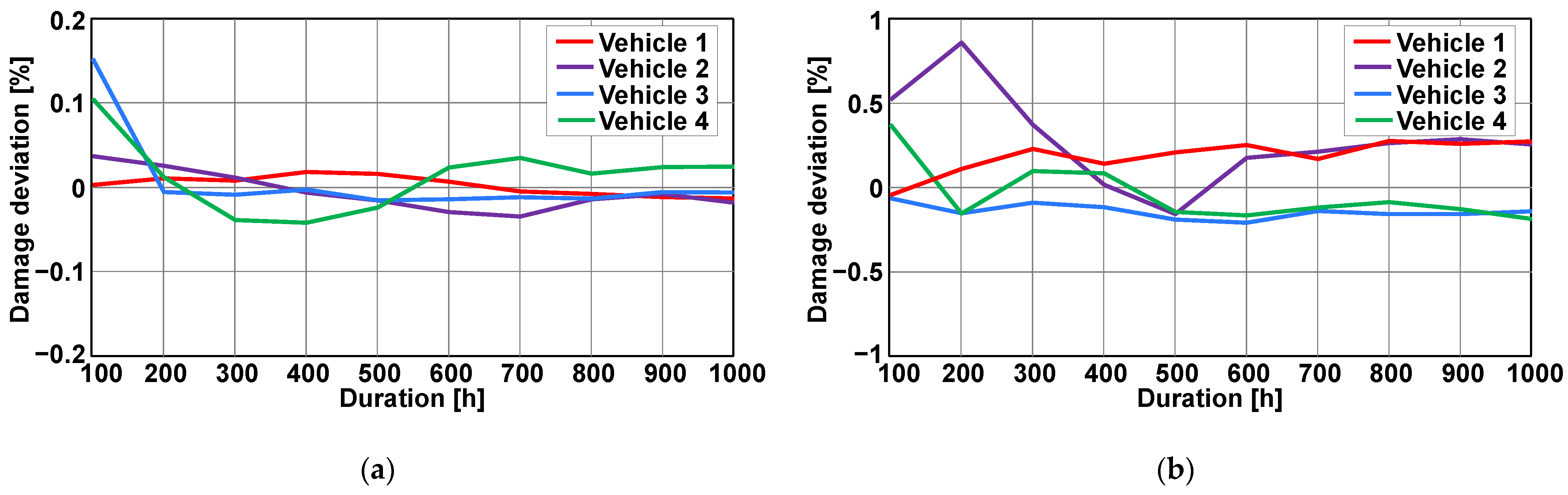
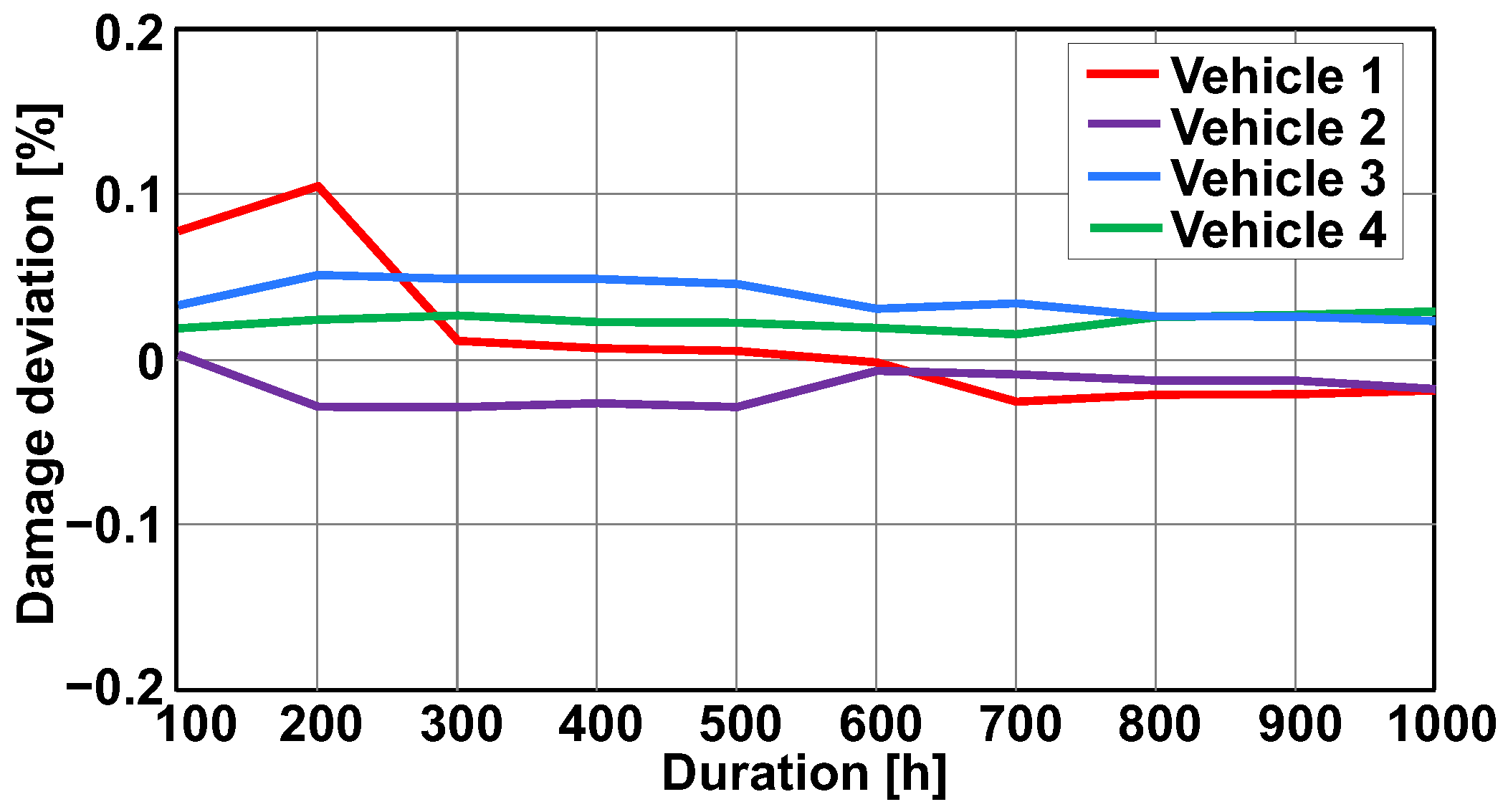
3.3. Significance of Low-Frequency Data for the Time at Level Classification

The investigation of the significance of low-frequency data for the time at level classification involves scaling the collectives to a duration of 8000 h. In this section, we evaluate the electromagnetic power with the original frequency of 100 Hz and the pulse inverter temperature originally at 2 Hz to obtain the collectives. The damage is calculated using fictitious Wöhler parameters. Figure 12 displays the damage deviations of the time at level classification. The data can be used for this analysis with a reduced frequency. The damage deviation curve follows a similar trend to the rollover classification. The deviations of the 10 Hz data are presented with solid lines and remain consistently smaller than 0.2% after 100 operating hours in Figure 12a. Figure 12b represents the deviations in damage of 1 Hz data, which are higher but still at an acceptable level, smaller than 1%.

Referring to Figure 12, the level of significance is higher for this non-dynamic signal, as demonstrated in Figure 13. The low-frequency data can support the same conclusion as the original data. In general, low-frequency data can be used directly in the analysis with the time at level classification, contributing to efficient design.

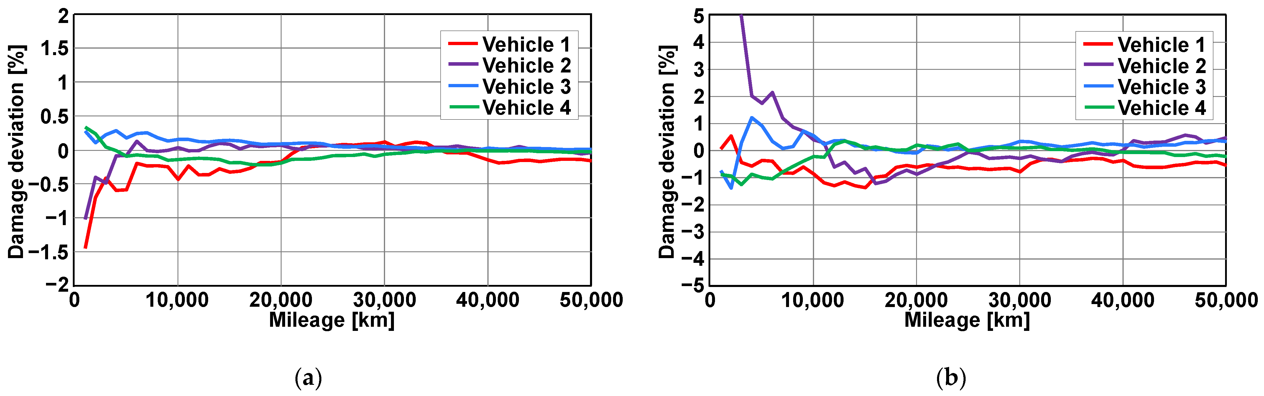
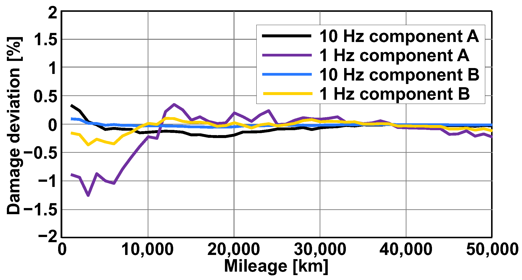
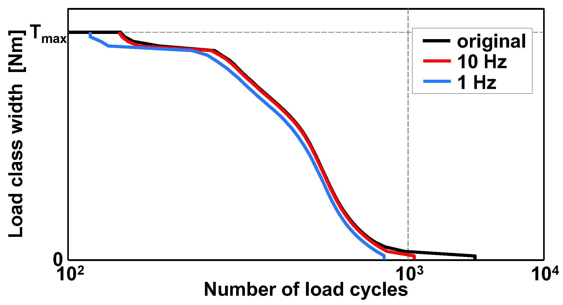
3.4. Significance of Low-Frequency Data for the Rainflow Classification

The rainflow classification is highly sensitive to information loss caused by downsampling, especially with the loss of load extremes. Figure 14 shows the collective from 10,000 km data, where the damage with 10 Hz is already approximately 5% lower than with 100 Hz. It is important to note that signal preprocessing can also miss the extremes.

Figure 15 displays the results for damage deviation with torque as the load in low frequency. The loss of the load hysteresis leads to significant damage deviations even with more data, particularly when the vehicle is driven by different people and in different driving environments with less repeatability. Therefore, reducing the frequency can result in a higher loss of information and deviation. The statement is no longer accurate. The torque data with low frequency cannot be used directly for rainflow classification.

Mildly reducing the frequency can result in smaller deviations. For example, in Figure 16, the damage caused by the rainflow classification for temperature at 1 Hz is approximately 2% lower than the damage caused by the original frequency of 2 Hz. However, deviations of over 6% can also occur, even when the data size is not small. The temperature readings are also influenced by the season and location, which impact the driving conditions. Driving in different regions leads to greater deviations due to varying environmental temperatures. Therefore, the use of low-frequency non-dynamic data in the rainflow analysis is restricted. The rainflow classification can be conducted using the online classification function in a vehicle, as explained in [15,40]. However, this method does not offer time series data to replicate the driving situation.

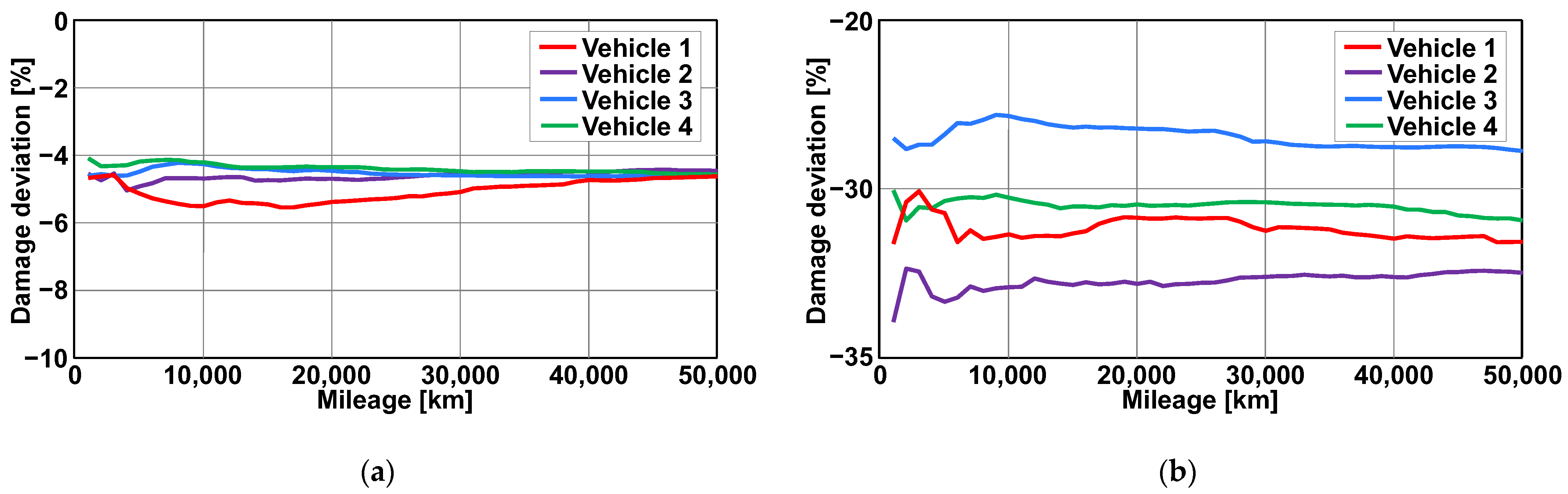
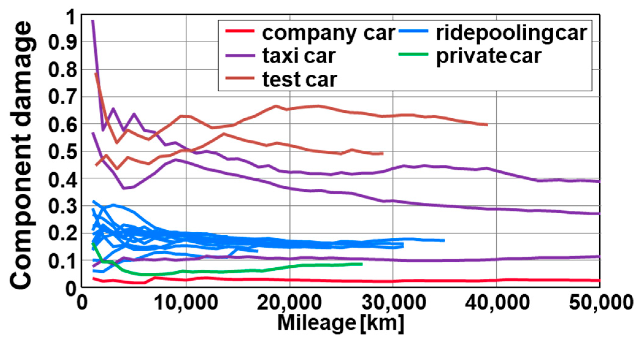
4. Statistical Stability of Data for Representative Damage

Another topic for discussion is the necessary data size for making statistically stable statements about component damage when important information, such as the number of drivers operating the vehicle in different driving environments, is unavailable. Generally, a larger amount of driving data, which provides more information about actual usage, leads to a more precise estimate of the component’s lifetime damage. Figure 17 shows the variability of relative component damage in relation to the damage incurred after 50,000 km of data with different data sizes. The data were divided into segments ranging from 1000 km to 25,000 km, and the damage was calculated for each segment to determine the dispersion. The box chart displays the interquartile range, which represents the middle 50% of the data. Vehicle 1 was driven by multiple drivers, resulting in a wider range of driving behaviors and environments, leading to more outliers. Each single result of vehicle 1 is shown with one square. However, with more data, the variance is reduced, which in turn reduces the influences of the driver and driving environment. Vehicles 2, 3, and 4 were driven by fewer drivers and in a more constrained environment, resulting in less variance compared to vehicle 1.

Figure 18 shows the normalized damages of seventeen vehicles, including one company car, three taxi cars, ten ridepooling cars, one private car, and two test cars. With the exception of ridepooling cars, all other vehicles are of the same type. This analysis focuses on these vehicles due to the variations in driver behavior and driven areas, which have significant impacts on the resulting damage. The influence of these factors can be observed by the position of the damage lines of the same type in Figure 17. Company cars are used by a diverse group of drivers in various areas, while taxi cars are driven by multiple drivers in different areas, but with a tendency towards sporty driving. The test cars are exclusively used on the testing ground by various drivers with different sporty driving styles. The 10 ridepooling cars are very similar to normal customer cars used for private family use, as they are driven by several drivers with limitations on driving style and areas. The private car was measured with a datalogger in the customer vehicle. This figure also illustrates the relationship between the data size and damage trend by displaying the calculated damages with different data sizes. The 10 ridepooling cars were evaluated directly with 10 Hz data on the cloud, while the other cars were driven by drivers with varying driving behaviors. As the data volume increases, the component’s variation exhibits a lower rate of change, indicating reduced volatility. Typically, a valid damage prediction can be achieved with 20,000 km of driving data for ridepooling cars, due to varying driver behaviors and driving environments, reaching a stable level. In contrast, taxi cars and the company car require more data to achieve a reasonable lifetime estimation. The dataset for the private passenger car displays the most significant regression. Data for vehicles with a driven distance of less than 5000 km may contain more contingencies due to drivers getting accustomed to the vehicle. However, other factors, such as the season and driver changes, can still influence the damage caused by usage. Therefore, data stability is also dependent on the scenarios. Durability research typically considers the stability of damage statements as a supplementary precondition.

The results of the paper indicate that low-frequency data can still provide reasonable statements when combined with signal classification to describe a certain repeatable component state, particularly when the data size is large enough. However, due to information loss, low-frequency data are generally unsuitable for describing state changes. The required data size to achieve a relatively stable level is significantly affected by the amount of repetition, which is influenced by the diver style and drive situations.

Table 2. The analysis results of the significance of low-frequency data and the minimum amount of data required for acceptable significance.

Classification	Signal	10 Hz	1 Hz
Rollover	EM Torque and Speed	5000 km	5000 km
Time at level	EM Power	100 h	100 h
Time at level	Pulse Inverter Temperature	-	100 h
Rainflow	EM Torque	Not possible	Not possible
Rainflow	Pulse Inverter Temperature	-	Limited

shows the general results of the significance analyses of the low-frequency data and the minimum number of data required to achieve acceptable significance in the present study, as analyzed in Section 3 and Section 4.

5. Conclusions

This paper examines the importance of low-frequency data in the development of durability. The study uses a database from four vehicles, each with over 50,000 km of real driving measurement data. Load collectives with different signal classifications were derived for the damage calculation, along with the corresponding Wöhler lines. To determine the significance of the deviation between the original high-frequency data and the downsampled data, a comparison was conducted. To be considered significant, the deviation must be less than 2%. The study also took into account the influence of preprocessing and the Wöhler line. The results suggest that reducing the data frequency to 1 Hz is sufficient for the rollover classification in the durability analysis. Preprocessing does not seem to have a significant impact on the results. The inclination of the Wöhler line has a notable effect on the significance. The statements for the time at level classification are similar. When using the rainflow classification, reducing the frequency results in a decrease in the level of significance. Therefore, it cannot provide a plausible conclusion for the durability analysis. To record the load extremes, an online classification function is required for rainflow classification, such as the onboard classification [15] or Porsche driving reflection module [40]. The statistical stability of representative damage prediction was analyzed using rollover results as an example. The size of the data has a direct impact on the accuracy of the damage prediction. The amount of data required is dependent on the usage of the vehicle.

Additional investigations are required for further development in durability regarding data significance and customer load collectives. For example, the database can be extended with more customer cars in different markets. To obtain clearer statements regarding the representative driver, it is recommended to increase the sample size. Additionally, low-frequency cloud data can be used to derive the typical testing circle directly. To enhance the depth of information, artificial intelligence methods such as deep learning can be considered, which are increasingly utilized in powertrain development [41]. Additionally, data quality can be improved through data fusion. By combining driving data with aided simulation, the driving situation can be reconstructed, resulting in higher quality data.

References

1. Sanguesa, J.A.; Torres-Sanz, V.; Garrido, P.; Martinez, F.J.; Marquez-Barja, J.M. A review on electric vehicles: Technologies and challenges. Smart Cities 2021, 4, 372–404. [Google Scholar] [CrossRef]
2. Wahid, M.R.; Budiman, B.A.; Joelianto, E.; Aziz, M. A review on drive train technologies for passenger electric vehicles. Energies 2021, 14, 6742. [Google Scholar] [CrossRef]
3. Shu, X.; Yang, W.; Guo, Y.; Wei, K.; Qin, B.; Zhu, G. A reliability study of electric vehicle battery from the perspective of power supply system. J. Power Sources 2020, 451, 227805. [Google Scholar] [CrossRef]
4. Liu, Z.; Tan, C.; Leng, F. A reliability-based design concept for lithium-ion battery pack in electric vehicles. Reliab. Eng. Syst. Saf. 2015, 134, 169–177. [Google Scholar] [CrossRef]
5. Shu, X.; Guo, Y.; Yang, W.; Wei, K.; Zhu, Y.; Zou, H. A detailed reliability study of the motor System in pure electric vans by the approach of fault tree analysis. IEEE Access 2019, 8, 5295–5307. [Google Scholar] [CrossRef]
6. Tang, Q.; Shu, X.; Zhu, G.; Wang, J.; Yang, H. Reliability study of BEV powertrain system and its components—A case study. Processes 2021, 9, 762. [Google Scholar] [CrossRef]
7. Tischmacher, H. Systematische Systemanalysen zur Elektrischen Belastung von Wältlagern bei Umrichtergespeisten Elektromotoren. Ph.D. Thesis, Universität Hannover, Hannover, Germany, 2017. [Google Scholar]
8. Horst, M.; Schäfer, U.; Schmidt, R. Ermittlung von statistisch abgesicherten Kunden-Lastkollektiven für Personenkraftwagen. In DVM-Bericht Nr. 129; Fahrwerke und Betriebsfestigkeit: Osnabrück, Germany, 2002. [Google Scholar]
9. Schimanski, S.; Barta, M.; Schröder, T.-F. Entwicklung eines autonomen Datenloggers zur Erfassung von Bewegungsdaten bei Elektro-Pkws für die Ableitung von nutzungszentrierten Dienstleistungsinnovationen. In Innovative Produkte und Dienstleistungen in der Mobilität; Springer Gabler: Wiesbaden, Germany, 2017. [Google Scholar]
10. Wagner, M. Dataloggerbasierte Kundenkollektivermittlung für die Fahrzeugerprobung. Ph.D. Thesis, Technische Universität Braunschweig, Braunschweig, Germany, 2017. [Google Scholar]
11. Pötter, K.; Till, R.; Horst, M. Kundenrelevante Betriebslasten—Neue Werkzeuge zur Ermittlung von Fahrzeuglasten im Kundenbetrieb. In DVM-Bericht Nr. 137; Auslegungs-und Absicherungskonzepte der Betriebsfestigkeit—Potenziale und Risiken: München, Germany, 2010. [Google Scholar]
12. Grünitz, K.; Manz, H.; Meyer, S. Ermittlung der Betriebsbelastungen elektromechanischer Lenkgetriebe mittels belastungserfassender Software. In DVM-Bericht Nr. 134; Lastannahmen und Betriebsfestigkeit: Wolfsburg, Germany, 2007. [Google Scholar]
13. Karspeck, T.; Klaiss, T.; Zellbeck, H. Reconstruction of Customer-Oriented Driving States by Efficient Data Storage on the Control Unit. In 9. Internationales Stuttgarter Symposium; Automobil-und Motorentechnik: Stuttgart, Germany, 2009. [Google Scholar]
14. Grober, F.; Janssen, A.; Küçükay, F. Bedarfsgerechte Lastannahme für Fahrzeugbauteile auf Basis von Kunden-Felddaten. In DVM-Bericht Nr. 146; Lastannahmen und Anforderungsmanagement in der Betriebsfestigkeit—neue Trends: Wolfsburg, Germany, 2019. [Google Scholar]
15. Grober, F. Optimierte Fahrzeugerprobung auf Basis von Kunden-Felddaten. Ph.D. Thesis, Technische Universität Braunschweig, Braunschweig, Germany, 2022. [Google Scholar]
16. Ehrich, F. Big Data as Enabler for Customer-Oriented Automotive Development. Master’s Thesis, Technische Universität Wien, Vienna, Austria, 2018. [Google Scholar]
17. Wöhler, A. Über Versuche zur Ermittlung der Festigkeit von Achsen. In Zeitschrift für Bauwesen; 1863; Volume 13, pp. 583–616. [Google Scholar]
18. Haibach, E. Betriebsfestigkeit: Verfahren und Daten zur Bauteilberechnung; VDI Verlag: Düsseldorf, Germany, 1989. [Google Scholar]
19. Miner, M.A.A. Cumulative damage in fatigue. Trans. J. Appl. Mech. 1945, 12, A159–A164. [Google Scholar] [CrossRef]
20. Palmgren, A. Die Lebensdauer von Kugellagern. In VDI-Zeitschrift, Nr. 68; 1924. [Google Scholar]
21. Hanisch, L.; Henke, M. Lifetime modelling of electrical machines using the methodology of design of experiments. Simul. Notes Eur. 2021, 31, 95–100. [Google Scholar] [CrossRef]
22. Köhler, M.; Jenne, S.; Pötter, K.; Zenner, H. Load Assumption for Fatigue Design of Structures and Components; Springer-Verlag GmbH: Berlin/Heidelberg, Germany, 2017. [Google Scholar]
23. Matsuishi, M.; Endo, T. Fatigue of metals subjected to varying stress. Jap. Soc. Mech. Engin. Fukuoka/Jpn. 1968, 68, 37–40. [Google Scholar]
24. Forschungsvereinigung Antriebstechnik, e.V. Zählverfahren zur Bildung von Kollektiven und Matrizen aus Zeitfunktionen; FVA-Richtlinie: Frankfurt, Germany, 2018. [Google Scholar]
25. Wang, Y.; Han, X.; Xu, X.; Pan, Y.; Dai, F.; Zou, D.; Lu, L.; Ouyang, M. A comprehensive data-driven assessment scheme for power battery of large-scale electric vehicles in cloud platform. J. Energy Storage 2023, 64, 107210. [Google Scholar] [CrossRef]
26. Song, L.; Zhang, K.; Liang, T.; Han, X.; Zhang, Y. Intelligent state of health estimation for lithium-ion battery pack based on big data analysis. J. Energy Storage 2020, 32, 101836. [Google Scholar] [CrossRef]
27. Zhang, J.; Wang, Z.; Liu, P.; Zhang, Z. Energy consumption analysis and prediction of electric vehicles based on real-world driving data. Appl. Energy 2020, 275, 115408. [Google Scholar] [CrossRef]
28. Corti, A.; Manzoni, V.; Savaresi, S.M. Vehicle’s energy estimation using low frequency speed signal. In Proceedings of the 15th International IEEE Conference on Intelligent Transportation Systems, Anchorage, AK, USA, 16–19 September 2012; pp. 626–631. [Google Scholar]
29. Shi, S.; Zhang, M.; Lin, N.; Yue, B. Low-cost reconstruction of typical driving cycles based on empirical information and low-frequency speed data. IEEE Trans. Veh. Technol. 2020, 69, 8221–8231. [Google Scholar] [CrossRef]
30. Zhang, J.; Wang, Z.; Liu, P.; Zhang, Z.; Li, X.; Qu, C. Driving cycles construction for electric vehicles considering road environment: A case study in Beijing. Appl. Energy 2019, 253, 113514. [Google Scholar] [CrossRef]
31. Noering, F. Unsupervised Pattern Discovery in Automotive Time Series. Ph.D. Thesis, Technische Universität Braunschweig, Braunschweig, Germany, 2021. [Google Scholar]
32. Heidenreich, N.; Opalinski, A.; Poll, G. Methode zur Analyse von Kundenkollektivmessungen mittels Einzelfahrtsegmentierung und Clusteralgorithmen. In Commercial Vehicle Technology 2020/2021; Springer Fachmedien Wiesbaden: Wiesbaden, Germany, 2021. [Google Scholar]
33. Sree Dhevi, A.T. Imputing missing values using Inverse Distance Weighted Interpolation for time series data. In Proceedings of the 2014 Sixth International Conference on Advanced Computing (ICoAC), Chennai, India, 17–19 December 2014; pp. 255–259. [Google Scholar]
34. Sidi, Y.; Harel, O. The treatment of incomplete data: Reporting, analysis, reproducibility, and replicability. Soc. Sci. Med. 2018, 209, 169–173. [Google Scholar] [CrossRef] [PubMed]
35. Ma, Q.; Gu, Y.; Lee, W.-C.; Yu, G. Order-sensitive imputation for clustered missing values. IEEE Trans. Knowl. Data Eng. 2019, 31, 166–180. [Google Scholar] [CrossRef]
36. Zhao, M.; Li, Y.; Chen, S.; Li, B. Missing value recovery for encoder signals using improved low-rank approximation. Mech. Syst. Signal Process. 2020, 139, 106595. [Google Scholar] [CrossRef]
37. Lepot, M.; Aubin, J.-B.; Clemens, F.H.L.R. Interpolation in Time Series: An Introductive Overview of Existing Methods, Their Performance Criteria and Uncertainty Assessment. Water 2017, 9, 796. [Google Scholar] [CrossRef]
38. Wegener, J.; van Putten, S.; Neubeck, J.; Wagner, A. Data Mining as an Enabler for Customer Data Driven Vehicle Development. In Proceedings of the Shanghai-Stuttgart-Symposium, Automotive and Powertrain Technology, Shanghai, China, 21–22 October 2021. [Google Scholar]
39. Anagnostopoulos, G.; Stavropoulos, G.; Violos, J.; Leivadeas, A.; Varlamis, I. Enhancing Virtual Sensors to deal with Missing Values and Low Sampling Rates. In Proceedings of the 2023 11th IEEE International Conference on Mobile Cloud Computing, Services, and Engineering (MobileCloud), Athens, Greece, 17–20 July 2023; pp. 39–44. [Google Scholar]
40. Porsche: Digitalisation of Vehicle Development. Available online: https://newsroom.porsche.com/en/2019/digital/porsche-digitalisation-vehicle-development-examples-16982.html (accessed on 21 January 2024).
41. Mirfendreski, A. Powertrain Development with Artificial Intelligence; Springer: Berlin/Heidelberg, Germany, 2022. [Google Scholar]
Figure 1. Wöhler line for the lifetime calculation with torque as the load.
Wevj 15 00088 g001
Figure 2. Rollover classification with defined torque classes from 1 to 6 and the time interval Δ t .
Wevj 15 00088 g002
Figure 3. Time at level classification with defined load classes from 1 to 6 and the time interval Δ t .
Wevj 15 00088 g003
Figure 4. Rainflow classification with defined torque classes from 1 to 7 and load extremes from A to L.
Wevj 15 00088 g004
Figure 5. Online data collection in a vehicle.
Wevj 15 00088 g005
Figure 6. EM torque for 3 s from the selected data. (a) The original torque and the torque after downsampling; (b) classified EM torques at different frequencies with 10 Nm as the class width.
Wevj 15 00088 g006
Figure 7. EM speed for 3 s from the selected data.
Wevj 15 00088 g007
Figure 8. Exemplary results of the rollover classification. (a) Rollover classification for the data of 10,000 km; (b) rollover classification for the data of 50,000 km.
Wevj 15 00088 g008
Figure 9. Damage deviation of the rollover classification. (a) Damage deviation of the rollover classification with 10 Hz data; (b) damage deviation of the rollover classification with 1 Hz data.
Wevj 15 00088 g009
Figure 10. Damage deviation of the rollover classification after signal preprocessing. (a) Vehicle 1; (b) vehicle 2; (c) vehicle 3; (d) vehicle 4.
Wevj 15 00088 g010
Figure 11. Impact of the Wöhler line on the damage deviation of the rollover classification.
Wevj 15 00088 g011
Figure 12. Damage deviation of the time at level classification for EM power. (a) Damage deviation of the time at level classification for EM power with 10 Hz data; (b) damage deviation of the time at level classification for EM power with 1 Hz data.
Wevj 15 00088 g012
Figure 13. Damage deviation of the time at level classification data significance for pulse inverter temperature.
Wevj 15 00088 g013
Figure 14. Rainflow classification for torque with 10,000 km data in the range pair format.
Wevj 15 00088 g014
Figure 15. Damage deviation of the EM torque rainflow classification. (a) Damage deviation of the EM torque rainflow classification with 10 Hz data; (b) damage deviation of the EM torque rainflow classification with 1 Hz data.
Wevj 15 00088 g015
Figure 16. Damage deviation of the temperature rainflow classification.
Wevj 15 00088 g016
Figure 17. Damage variability of the data with different data sizes.
Wevj 15 00088 g017
Figure 18. Component damages in relation to the data size.
Wevj 15 00088 g018