Article

Research on Longitudinal Control Algorithm of Adaptive Cruise Control System for Pure Electric Vehicles

College of Automotive Engineering, Jilin University, Changchun 130022, China
*
Author to whom correspondence should be addressed.
World Electr. Veh. J. 2023, 14(2), 32; https://doi.org/10.3390/wevj14020032
Submission received: 30 November 2022 / Revised: 25 January 2023 / Accepted: 26 January 2023 / Published: 28 January 2023

Abstract

:
The vehicle longitudinal control algorithm is the core function of the adaptive cruise control system, whose main task is to convert vehicle acceleration and deceleration requirements into vehicle driving and braking commands so that the vehicle can quickly and accurately track the desired acceleration. Traditional longitudinal control algorithms rely on accurate vehicle dynamic modeling or complex controller parameter calibrations. To overcome those difficulties, a longitudinal control algorithm based on RBF-PID is proposed in this paper. The algorithm uses the RBFNN (radial basis function neural network), which can simply and quickly approximate any complex nonlinear system, to identify the Jacobian information of the vehicle and perform parameter tuning for PID control and achieve vehicle longitudinal control with self-tuning capability. Finally, the algorithm of this paper is verified by the joint simulation of Matlab/Simulink and Carsim. The results show that this algorithm has a better response rate and anti-jamming capability than the traditional PID control and can achieve accurate and rapid tracking of the desired acceleration.

1. Introduction

With the rapid growth of production and ownership of automobiles, problems such as environmental pollution, resource shortage [1], and traffic congestion that constrain economic development are becoming more and more serious [2]. A large amount of greenhouse gas emissions from automobiles is one of the major contributors to global climate change and is considered one of the most serious challenges facing sustainable development [3]. Meanwhile, advanced driver assistance systems (ADAS) are treated as an effective way to solve the above problems ADAS can better protect us from some of the human factors, and human error is the cause of most traffic accidents [4]. ADAS develops to understand human behavior as well as to monitor health status [5] and potentially improve fuel consumption and safety along with awareness of external driving conditions [6]. Besides, ADAS can also be applied to pure electric vehicles to optimize the driving experience [7].
Adaptive cruise control (ACC), one of the core functions of ADAS equipment, can monitor road conditions in real-time and control vehicle speed and acceleration on its own, which helps to save resources and ensure vehicle safety [8,9]. ACC systems are often designed to be hierarchical, including three layers of perception, decision, and execution. The decision algorithm uses environmental information obtained from the perception layer and the state information of the vehicle itself to calculate the target acceleration. The vehicle longitudinal control algorithm is in the execution layer and is responsible for converting the target acceleration into demand driving and braking torque [10]. Due to the strong coupling and nonlinear characteristics of the vehicle longitudinal dynamic systems, how to quickly and accurately obtain the mapping relationship is a critical and technical difficulty that needs to be solved for the vehicle longitudinal control algorithm. Current researchers’ analysis of the mapping relationship is divided into the following two main categories: model control and non-model control.
In model-based control, some scholars built vehicle models to perform dynamics control. Fritz used state-space equations to model the vehicle system and used a nonlinear controller to control the vehicle model [11,12]. The 14 degrees of freedom (DOF) longitudinal dynamics model of the Toyota Rav4EV 2012 was developed in the MapleSim by Batra. M et al. software using the estimated parameters. The accuracy of the identified parameters and the model was validated by comparing the model output against the experimental data [13]. While in terms of non-model control, the main algorithms include classical PID control, data look-up table, intelligent control, etc. Some scholars use PID control methods. P. Shakouri et al. linearized the nonlinear dynamic models of the vehicle at the selected operating point and used a PI controller to complete the control of the throttle position [14]. Considering the nonlinear characteristics of the electronic throttle, Feng Daoning et al. used various PID algorithms such as incremental, integral separation, deadband, and feedforward compensation to improve the system response speed while reducing the static difference. Those algorithms have been verified through experimental bench and practical vehicle tests [15]. Some scholars use data lookup tables to follow the desired acceleration while avoiding the recognition accuracy of vehicle dynamic parameters affecting the control effect. Pei et al. established a three-dimensional look-up diagram of throttle opening-vehicle speed-acceleration in the driving process and cooperating with the control structure of feedforward plus proportional feedback to realize the control of the acceleration process. Then they established a three-dimensional look-up diagram of brake pressure-vehicle speed-deceleration in the braking process, cooperated with the control structure of feedforward plus integral feedback to realize the control of the braking process [16]. For intelligent control, Abdelkader El Kamel et al. used graded processing for longitudinal control and fuzzy control for throttle/brake control. Acceleration error and speed error as control inputs, while throttle opening variation and brake torque variation as control outputs. Finally, the speed/vehicle distance following effect and the robustness under the external environmental disturbance were verified for the control method [17]. A fuzzy longitudinal control system was proposed by Ching-Chih Tsai et al. The input of the fuzzy longitudinal controller included the safety distance, actual vehicle distance, and relative vehicle speed, and the output PWM signal controlled the output force of the vacuum booster. The control algorithm has been tested in the Simulink simulation platform at low-speed and high-speed conditions [18]. A robust control strategy based on nonlinear model predictive control and Takagi-Sugeno (TS) fuzzy model was proposed by Khooban et al., which was evaluated for various operating conditions of electric vehicles [19]. To perform adaptive speed control for highly nonlinear hybrid electric vehicles (HEVs) equipped with the electronic throttle control system, Kumar et al. proposed fractional-order fuzzy PD (FOFPD) controller and fractional-order fuzzy PI (FOFPI) controller as the primary and secondary controllers of the cascade control loop, respectively [20].
It should be noted that the above control algorithms have limitations in their application. Although the algorithm based on model control can reduce the number of comparisons, it requires high modeling accuracy and accuracy of model parameters. In terms of non-model control, the algorithm of classical PID control is stable, easy to adjust, and does not depend on an accurate vehicle model. However, for nonlinear time-varying systems, conventional PID control with three fixed parameters is difficult to meet the requirements [21]. The look-up tables require extensive calibration experiments and long development cycles, with bad portability. Intelligent control algorithms are complex and have a great deal of calculation, so they are currently seldom used in practical applications. Most of the longitudinal dynamics control methods are based on the vehicle body characteristics to adjust the PID parameters or other control rules. If the external environment (slope, wind speed, etc.) changes, it will have a great impact on the vehicle acceleration control accuracy. At present, the longitudinal dynamics control algorithm for conventional engine vehicles with adaptive cruise has been studied more. The longitudinal dynamics control algorithm for pure electric vehicles is less researched. For the pure electric vehicle adaptive cruise control system, the drive control mechanism is a motor. If considering the braking energy recovery characteristics, the pure electric vehicle braking control mechanism includes the motor and hydraulic braking system. Compared with conventional vehicles, braking control is more complex [22]. Because the vehicle traction and brake system are very complex, with strong nonlinearity and coupling, it is difficult to establish a mathematical model to describe them accurately [23]. The current longitudinal dynamic systems control is developing toward model-free and self-learning [24]. Neural network (NN), as an intelligent algorithm with strong self-learning, self-adaptive and self-organizing capabilities, is outstanding in the control of nonlinear systems [25]. The prediction model built by RBFNN can approximate any nonlinear function with arbitrary accuracy and has the advantages of simple structure and fast convergence [26]. It provides a new idea for vehicle longitudinal control.
A longitudinal control algorithm applied to the ACC system for the pure electric vehicle is proposed in this paper. The control method in this paper is a control algorithm with adaptive capability. It optimizes the current control input based on past inputs and the effect of the error following. The control method does not require an exact model of the system itself and is highly adaptable to nonlinear and time-varying systems. The outputs of the algorithm are the motor torque and total brake torque demands for driving and braking, which are sent to the vehicle model so that the host vehicle can accurately track the desired acceleration. If considering the braking energy recovery characteristics, the pure electric vehicle braking control mechanism includes the motor and hydraulic braking system. The total braking force demanded by the algorithm output can be used for regenerative braking system design for the next step of braking force distribution, including front and rear axle braking force distribution and hydraulic braking force, and motor regenerative braking force distribution. It expands the application range of adaptive cruise control systems and improves the performance index of the adaptive cruise control system. Compared with the current work, the main contributions of this paper are as follows. The RBFNN is introduced into the traditional PID control to realize the longitudinal control with self-adjustment capability. The learning ability of RBFNN is applied to identify the vehicle longitudinal dynamic systems and fine-tune the PID control parameters according to the control effect. The control method in this paper can accurately and quickly convert the target acceleration into the demand driving and braking torque, achieving accurate tracking of the target acceleration with high robustness and portability. The rest of this paper is organized as follows. Section 2 describes the vehicle platform and the control framework and explains the longitudinal control algorithm based on RBFNN tuning PID control. Simulation results and discussion are discussed in Section 3. Lastly, conclusions are drawn in Section 4.

2. Materials and Methods

2.1. Vehicle Platform and Control Framework

2.1.1. Vehicle Platform

As shown in Figure 1, the adaptive cruise longitudinal control algorithm proposed in this paper is deployed on a front-wheel-drive electric vehicle. In addition to being equipped with radars to detect the moving obstacles ahead, the vehicle’s traction system contains a permanent magnet synchronous motor with a motor control unit (MCU), transmission, and differential. The vehicle is also equipped with a high-voltage battery pack and battery management system (BMS) to provide energy for the motor. The traction system model, which accepts the desired motor torque and outputs the actual motor torque, is established by Matlab/Simulink. The hydraulic brake system is established by Matlab/Simulink, which contains the master cylinder, hydraulic regulation unit, disc brakes equipped on each wheel, and brake control unit (BCU). BCU controls the solenoid valves in the hydraulic regulation unit according to the desired pressure and outputs the hydraulic braking torque. The vehicle dynamic model established by Carsim contains the wheel, suspension, and spring-loaded mass models, which accept the actual motor torque and hydraulic braking torque. At the same time, the vehicle dynamic model feeds the vehicle status back to the ACC controller. When the ACC system works, the ACC controller continuously calculates the vehicle’s accelerating and braking demands based on the environmental information from the radars. The MCU and BCU receive the corresponding commands from the ACC system and control the actuators to execute. The specific vehicle model development process will not be discussed here.

2.1.2. Control Framework

The fundamental function of the ACC system is to automatically regulate the host vehicle’s speed to maintain safe vehicle spacing from the lead vehicle. As shown in Figure 2, the control framework of the pure electric vehicle ACC system is designed to be hierarchical. In the control framework, the perception layer algorithm analyzes the relative state of the host vehicle to the lead vehicle based on the radar signal and the vehicle signal; the decision algorithm identifies the sliding acceleration and calculates the target acceleration to determine whether the car is in driving or braking state according to the mode switching logic [27]. The above algorithms are not introduced in this paper. The inputs of the pure electric vehicle adaptive cruise longitudinal control algorithm designed in this paper are the target acceleration a t a r g e t and the actual acceleration of the vehicle a v e h . Then, RBFNN is used to identify the vehicle system and calculate the adjustment quantity of the PID parameters to obtain the PID parameters that are continuously optimized. The outputs of the algorithm are the motor torque T m o t o r _ d r i v e _ r e q and total brake torque T b r a k e _ a l l _ r e q demands for driving and braking, which are sent to the vehicle model so that the host vehicle can accurately track the desired acceleration. The vehicle platform has been described in detail in Section 2.1.1.

2.2. RBFNN-PID-Based Longitudinal Control Algorithm

Along with the problem of difficulty in building accurate mathematical models, it is difficult to achieve accurate control of nonlinear time-varying systems. Classical PID control usually fails to implement the ideal control effect.
In the parameter self-tuning method of PID, the early rule-based and model-based PID parameter self-tuning has gradually become unsuitable for complex control conditions. With the development of intelligent control technology and advanced algorithm research, intelligent PID controller has attracted a lot of attention [28]. Among them, the expert adjusts the PID parameters by storing the real-time acquired measurement data and historical experience data in the database, and then selects the optimal parameters based on the heuristic reasoning mechanism [29]. The shortcomings of expert PID control are a large amount of calculation and the difficulty of obtaining empirical data. The fuzzy PID control method also relies on the adjustment experience and technical knowledge of the operator or expert and summarizes them into a fuzzy rule model. Self-adjustment of PID parameters is realized by using fuzzy reasoning [30]. The use of genetic algorithm can optimize the PID control parameters according to the output of the controlled object without knowing all the information of the controlled object, and the global optimal solution can be found by using the population optimization mechanism, but there is a disadvantage of slow convergence [31]. In the control method based on neural network tuning PID, the widely used ones are mainly BP neural network and RBF neural network. Both BP and RBF are structurally divided into input, output, and hidden layers. The difference is that the BP neural network may have multiple hidden layers, while the RBF has a single hidden layer. In the case of the same number of nodes in the hidden layer, the approximation effect of RBF is better than that of BP, and the structure of BP neural network is more complex than that of RBF with the same number of samples and accuracy requirements. Considering the slow convergence speed of BP neural network and the problem of local optimal solution, the RBF neural network with higher approximation accuracy and faster convergence speed is used to adjust the PID controller parameters online in real time [32].
Neural networks can be trained to approximate arbitrary complex nonlinear systems. In this section, RBFNN is used to identify the Jacobian information of the controlled object, and the gradient descent algorithm is used to calculate the adjustment quantity of the PID parameters to obtain the continuously optimized PID parameters. The parameter-tuned PID controller can adapt to environmental changes, making it have strong robustness and high control accuracy for nonlinear systems. Finally, a pure electric vehicle adaptive cruise longitudinal control algorithm is designed based on RBFNN tuning PID control.

2.2.1. Parameter Tuning of RBFNN-Based PID

PID control can realize the control of the error of the controlled system, with the characteristics of simple algorithm structure and better robustness. The current commonly used PID control method is digital PID control, which is divided into positional PID control and incremental PID control, both of which use the deviation values of different sampling points as control inputs.
The equation of the positional PID control is shown in Equation (1), which has a great deal of calculation due to the need for the accumulation process of e ( k ) .
u ( k ) = K p { e ( k ) + T T I j = 0 k e ( j ) + T D T [ e ( k ) e ( k 1 ) ] } ,
As shown in Equation (2), the essence of incremental PID control is not the control quantity for the target, but the increment of the control quantity. Therefore, the incremental PID control that facilitates quick results of requirements is less affected by system error disturbances and has little calculation.
{ Δ u ( k ) = K p Δ e ( k ) + K I e ( k ) + K D [ Δ e ( k ) Δ e ( k 1 ) ] Δ e ( k ) = e ( k ) e ( k 1 ) u ( k ) = u ( k 1 ) + Δ u ( k ) ,
Classical PID controllers are usually used to calibrate time-invariant systems, resulting in fixed proportional-integral-differential coefficients. For nonlinear time-invariant systems, the parameter calibration process using classical PID control methods is more complex and requires extensive experience of the operators, whose control effect that can be achieved is far from the ideal effect with the problem of control overshoot. The neural network algorithm is outstanding in nonlinear system control, so it can be used to identify the nonlinear system and continuously optimize the PID parameters. Thus, this paper proposes PID control based on RBFNN tuning for the design of a longitudinal control algorithm.
In this paper, the PID control based on RBFNN tuning is shown in Figure 3. By processing the input and output information of the controlled object, the PID proportional-integral-differential coefficients are continuously optimized to make the actual output of the controlled object as fast and smooth as possible to approach the control target output.
The incremental PID control algorithm was selected to facilitate the optimal design of the PID coefficients by RBFNN. The control error can be expressed as follows:
e r r o r ( k ) = r i n ( k ) y o u t ( k ) ,
The rectification index of the neural network is selected, as shown in Equation (4).
E ( k ) = 1 2 e r r o r ( k ) 2 ,
The adjustment quantity of the PID parameters are calculated using the gradient descent algorithm as follows:
Δ k p = η k E k p = η k E y y Δ u Δ u k p = η k e r r o r ( k ) y Δ u x c ( 1 ) ,
Δ k i = η i E k i = η i E y y Δ u Δ u k i = η i e r r o r ( k ) y Δ u x c ( 2 ) ,
Δ k d = η d E k d = η d E y y Δ u Δ u k d = η d e r r o r ( k ) y Δ u x c ( 3 ) ,
where y Δ u is the Jacobian information of the controlled object, η p , η i , η d is the learning rate of PID parameters, x c ( 1 ) = e r r o r ( k ) e r r o r ( k 1 ) , x c ( 2 ) = e r r o r ( k ) , x c ( 3 ) = e r r o r ( k ) 2 e r r o r ( k 1 ) + e r r o r ( k 2 ) .
Based on the above work, the coefficients correction results were obtained as follows:
{ k p ( k ) = Δ k p + k p ( k 1 ) k i ( k ) = Δ k i + k i ( k 1 ) k d ( k ) = Δ k d + k d ( k 1 ) ,

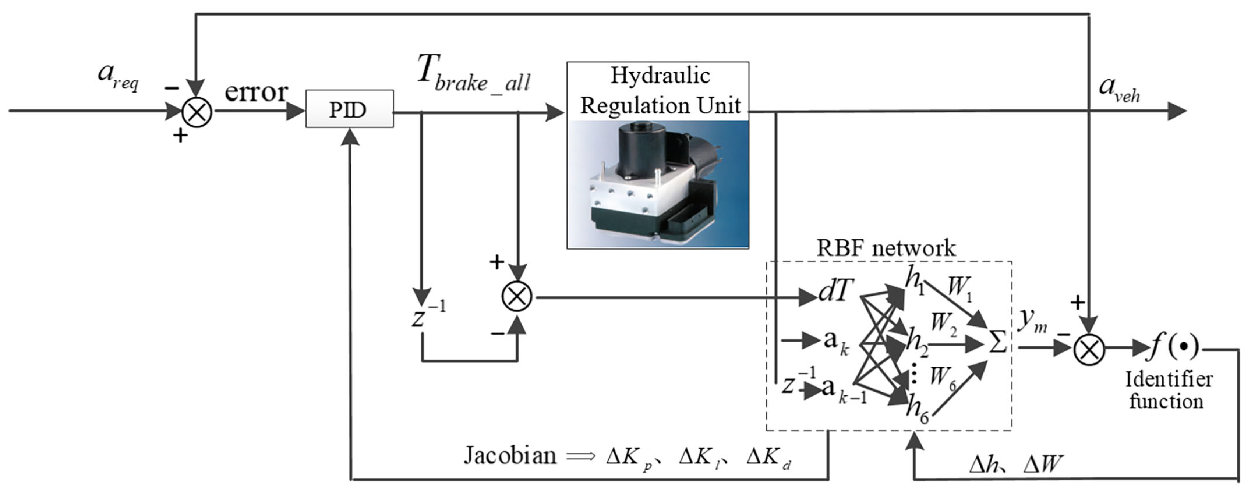
2.2.2. Jacobian Information Recognition Based on RBFNN

Based on the research content of the previous section, it is known that if we obtain the real-time optimized feature parameters, then the Jacobian information of the controlled object needs to be obtained. Next, this paper will achieve the recognition of Jacobian information of the controlled object based on RBFNN.
The RBF network is a three-layer feedforward network, including an input layer, a hidden layer, and an output layer, in which the transformation from the input layer to the hidden layer is nonlinear. The commonly used activation function of the hidden layer is the Gaussian function, as shown in Equation (10), and the hidden layer to the output layer of the RBF neural network is a linear transformation, as shown in Equation (13). The RBFNN structure is shown in Figure 4. RBF learning methods mainly include the k-means method, OLS (orthogonal least squares), and gradient descent method [33], etc. In the current RBF neural network application, the number of neurons in the hidden layer can be selected empirically. In addition, there are three other parameters that need to be learned in the network, namely, the center vector of the radial basis function, the width of the basis function, and the weight of each connection from the hidden layer to the output layer. In this paper, all three parameters are trained using supervised learning methods, and all parameters undergo an error correction learning process, and the data taken for training is also the error between the target value and the actual value output by the system. In this paper, the gradient descent method is used. Then the iterative algorithm for the output weight, node center, and node base width parameters is calculated as shown in Equations (15)–(19).
In Figure 4, where X = [ x 1 , x 2 , , x n ] T is the input vector of the network, in this paper the input vector is chosen as follows:
X = [ d u , y k , y k 1 ] T ,
where d u is the input value difference between the current and previous cycle of the controlled object, y k is the output value of the current cycle, and y k 1 is the output value of the previous cycle.
The Radial basis vector of the RBF network is H = [ h 1 , h 2 , , h j , , h m ] T , where h j is the Gaussian basis function.
h j = exp ( X C j 2 2 b j 2 ) ( j = 1 , 2 , , m ) ,
The center vector of the j th node of the network is C j = [ c j 1 , c j 2 , , c j i , , c j n ] T , where i = 1 , 2 , , n .
Let the base width vector of the network be shown as follows:
B = [ b 1 , b 2 , , b m ] T ,
where b j is the base width parameter of node j.
The weight vector of the network is as follows:
W = [ w 1 , w 2 , w j , , w m ] T ,
The output of the identification network is as follows:
y m ( k ) = w 1 h 1 + w 2 h 2 + + w m h m ,
The performance function of the identifier is as follows:
J 1 = 1 2 ( y o u t ( k ) y m ( k ) ) 2 ,
According to the gradient descent algorithm, the iterative algorithm for the output weight, node center, and node base width parameters is calculated as follows:
w j ( k ) = w j ( k 1 ) + η ( y o u t ( k ) y m ( k ) ) h j + α ( w j ( k 1 ) w j ( k 2 ) ) ,
Δ b j = ( y o u t ( k ) y m ( k ) ) w j h j X C j 2 b j 3 ,
b j ( k ) = b j ( k 1 ) + η Δ b j + α ( b j ( k 1 ) b j ( k 2 ) ) ,
Δ c j i = ( y o u t ( k ) y m ( k ) ) w j x j c j i b j 2 ,
c j i ( k ) = c j i ( k 1 ) + η Δ c j i + α ( c j i ( k 1 ) c j i ( k 2 ) ) ,
where α is the momentum factor, η is the learning rate.
The Jacobian array is obtained as follows:
y ( k ) Δ u ( k ) y m ( k ) Δ u ( k ) = j = 1 m w j h j c j i x 1 b j 2 ,
where x 1 = Δ u ( k ) .

2.2.3. Longitudinal Control Algorithm

In the control framework, the perception layer algorithm analyzes the relative state of the host vehicle to the lead vehicle based on the radar signal and the vehicle signal; the decision algorithm identifies the sliding acceleration and calculates the target acceleration to determine whether the car is in driving or braking state according to the mode switching logic. The inputs of the pure electric vehicle adaptive cruise longitudinal control algorithm designed in this paper are the target acceleration and the actual acceleration of the vehicle. Then, RBFNN is used to identify the vehicle system and calculate the adjustment quantity of the PID parameters to obtain the PID parameters that are continuously optimized. The outputs of the algorithm are the motor torque and total brake torque demands for driving and braking, which are sent to the vehicle model so that the host vehicle can accurately track the desired acceleration. The pure electric vehicle in the driving process only needs to achieve the target acceleration tracking by controlling the motor drive torque. Thus according to the demand of the PID control algorithm based on RBFNN, as shown in Figure 5, the difference between the selected target acceleration a r e q and the current actual acceleration a v e h is selected as the control algorithm input, with the motor demand drive torque T m o t o r _ d r i v e _ r e q as the output of the driving process control algorithm.
When the braking system performs the braking response to track the target acceleration, it is necessary to first confirm the magnitude of the total demand braking torque T b r a k e _ a l l . Thus, the difference between the target acceleration a r e q and the actual acceleration a v e h can be selected as the control algorithm input and the total demand braking torque T b r a k e _ a l l as the control algorithm output, as shown in Figure 6, according to the demand of the RBFNN-tuned PID control algorithm.

3. Results and Discussion

In the driving and braking process control, to verify the effectiveness, fast response, and anti-jamming of the control algorithm, based on the research in Section 2, this paper uses Matlab/Simulink and Carsim platform to build the longitudinal control model based on RBFNN-PID, and verify the drive and brake control effect. The control method of this paper and the traditional PID control are used to simulate the braking system and drive system models by responding to step signals and fighting against external disturbances, and the control effects of both are compared to prove that the control method of this paper has better control effects.
To verify the effectiveness of the longitudinal control algorithm, several experiments are conducted utilizing Matlab/Simulink (v.9.5, MathWorks, Natick, MA, USA) and Carsim (v.2016, MSC, The Ann Arbor, MI, USA). The main parameters used in the simulations are set in Table 1.

3.1. Results and Discussion of the Driving Process

3.1.1. Step Response of the Driving Process

As shown in Figure 7, it can be seen that the initial vehicle speed is 10 km/h, and the vehicle speed increases continuously with a certain slope to respond to the target acceleration. The specific acceleration response effect is shown in Figure 8, and the control effect is evaluated in terms of system response rapidity and smoothness. The settling time, i.e., the time required to reach the allowable error range, is used to evaluate the rapidity of the system response. The settling time of the traditional PID control algorithm is 1.41 s, while the algorithm of this paper is 0.459 s. It can be seen that the response rate of this paper is significantly faster than the effect of traditional PID control. The maximum overshoot, which is the ratio of the difference between the maximum peak value and the steady-state value to the steady-state value, is used to evaluate the smoothness of the system response. The maximum overshoot of the conventional PID control algorithm is 39.9%, while the method in this paper is 6%. It can be seen that the response process of this algorithm is smoother. Because the vehicle traction and brake system are very complex, with strong nonlinearity and coupling, it is difficult to establish a mathematical model to describe them accurately. As for acceleration fluctuations after 5 s in Figure 8, due to the inevitable errors in the established motor and battery model system in Matlab/Simulink, the acceleration simulation results inevitably fluctuate, and it is hard to get close to the target value without error. The acceleration error variation is shown in Figure 8, and it can be seen that both control methods have almost no static difference under steady-state conditions. The control effect of the PID control based on RBFNN can meet the control requirements and has an excellent control effect in the driving process. In a contrast, the conventional PID controller parameters are set to similar values to the last stable value of the RBFPID controller parameters. The change in the coefficients of the RBFPID controller is shown in Figure 9, whose initial values are 0.2, 0, and 0. The parameter Ki was adjusted the fastest, reaching a stable value for the first time in 0.362 s, with a final stable value of 0.7094. Additionally, the parameter Kp and parameter Kd finally stabilized at 0.4213 and 0.0024, respectively.

3.1.2. Response under Perturbation of the Driving Process

As shown in Figure 10, an external disturbance of amplitude 0.5 m/s2 is added to the target acceleration at 10 s during the response of the drive system to the step signal. The vehicle speed rises essentially at a constant slope and is largely unaffected by disturbances. It can be seen from Figure 11 that the conventional PID takes 1.56 s to reach the steady state after the external disturbance, while the control method in this paper is shortened to 1.13 s, which shows a better anti-jamming performance.

3.2. Results and Discussion of the Braking Process

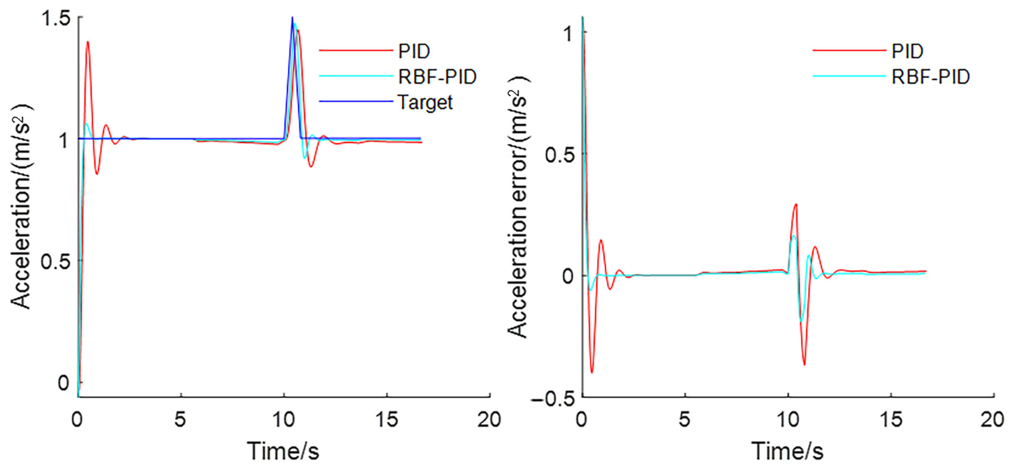
3.2.1. Step Response of the Braking Process

From Figure 12, it can be seen that the initial vehicle speed is 100 km/h, and the vehicle speed decreases continuously with a certain slope to respond to the target acceleration. The specific deceleration response effect is shown in Figure 13, and the system shows an overdamping state. Similarly, the settling time is used to evaluate the system response rapidity. The simulation results show that the settling time of the traditional PID is 1.051 s and the method of this paper is 0.521 s. Obviously, the response rate of the proposed algorithm in this paper is faster during the braking process. By observing the variation of acceleration error in Figure 13, it can be clearly seen that under steady-state conditions, both control algorithms have almost no static difference. The control effect of the PID control based on RBFNN can meet the control requirements and also has an excellent control effect for the braking process.

3.2.2. Response under Perturbation of the Braking Process

As shown in Figure 14, an external disturbance of amplitude 0.5 m/s2 is added to the target acceleration at 5 s during the response of the brake system to the step signal. As shown in Figure 14, the vehicle speed decreases essentially at a constant slope and is largely unaffected by disturbances. It can be seen from Figure 15 that the conventional PID takes 0.67 s to reach the steady state after the external disturbance, while the control method in this paper is shortened to 0.5 s, which also shows a better anti-jamming performance in the braking process.

4. Conclusions

The main performances in the simulations are shown in Table 2.
This paper proposes an adaptive cruise longitudinal control algorithm, specifically including the design of adaptive cruise driving and braking control algorithm based on RBFNN tuning PID control. Finally, a joint simulation using Matlab/Simulink and Carsim platforms is conducted to verify the target acceleration tracking effect in drive and brake control. The control algorithm of this paper and the traditional PID control were simulated separately to compare the control effects of both, whose conclusions were drawn as follows:
(1)
In response to the step signal in the driving case, the control method in this paper reaches the steady state with no static difference faster than the traditional PID control in the steady state condition, and the time required is reduced by about two-thirds. In addition, the maximum overshoot of this control algorithm is smaller, only about one-seventh of the traditional PID control, so the system response process is smoother. When adding disturbances, the control method used in this paper takes about three-tenths of the time to restore the steady state than the traditional PID control, showing a better anti-jamming ability;
(2)
In response to the step signal during the braking process, the response speed of this control algorithm is doubled compared with the traditional PID control. Similarly, when adding disturbances, this control algorithm takes less time to restore the steady state, which is about three-tenths less than the traditional PID control. The control algorithm has a better anti-jamming ability.
The control method in this paper is a control algorithm with adaptive capability. It optimizes the current control input based on past inputs and the effect of the error following. The control method does not require an exact model of the system itself and is highly adaptable to nonlinear and time-varying systems. The outputs of the algorithm are the motor torque and total brake torque demands for driving and braking, which are sent to the vehicle model so that the host vehicle can accurately track the desired acceleration. If considering the braking energy recovery characteristics, the pure electric vehicle braking control mechanism includes the motor and hydraulic braking system. The total braking force demanded by the algorithm output can be used for regenerative braking system design for the next step of braking force distribution, including front and rear axle braking force distribution and hydraulic braking force, and motor regenerative braking force distribution. By responding to step signals and fighting against external disturbances, the control algorithm in this paper exhibits higher robustness, better control accuracy, and stronger anti-jamming capability in driving and braking situations. It has proved that the adaptive cruise longitudinal control algorithm for pure electric vehicles proposed in this paper has a good control effect. It also expands the application range of adaptive cruise control systems and improves the performance index of the adaptive cruise control system.

Author Contributions

Conceptualization, L.C. and D.Z.; methodology, software, validation, H.L., Y.X., D.Z. and C.S.; investigation, resources, writing—original draft preparation, writing—review and editing, visualization; supervision; project administration, L.C., H.L., Y.X., D.Z. and C.S. All authors have read and agreed to the published version of the manuscript.

Funding

This research received no external funding.

Data Availability Statement

Not applicable.

Conflicts of Interest

The authors declare no conflict of interest.

References

  1. Gao, J.; Chen, H.; Li, Y.; Chen, J.; Zhang, Y.; Dave, K.; Huang, Y. Fuel consumption and exhaust emissions of diesel vehicles in worldwide harmonized light vehicles test cycles and their sensitivities to eco-driving factors. Energy Convers. Manag. 2019, 196, 605–613. [Google Scholar] [CrossRef]
  2. Li, Q.; Tian, S.; Wang, W. Environmental and Social Problems and Countermeasures in Transportation System under Resource Constraints. Complexity 2020, 2020, 6629119. [Google Scholar] [CrossRef]
  3. Liu, Z.; Feng, K.; Davis, S.J.; Guan, D.; Chen, B.; Hubacek, K.; Yan, J. Understanding the energy consumption and greenhouse gas emissions and the implication for achieving climate change mitigation targets. Appl. Energy 2016, 184, 737–741. [Google Scholar] [CrossRef] [Green Version]
  4. Ziebinski, A.; Cupek, R.; Grzechca, D.; Chruszczyk, L. Review of advanced driver assistance systems (ADAS). AIP Conf. Proc. 2017, 1906, 120002. [Google Scholar]
  5. Izquierdo-Reyes, J.; Ramirez-Mendoza, R.A.; Bustamante-Bello, M.R. A study of the effects of advanced driver assistance systems alerts on driver performance. Int. J. Interact. Des. Manuf. IJIDeM 2017, 12, 263–272. [Google Scholar] [CrossRef]
  6. Marina Martinez, C.; Heucke, M.; Wang, F.-Y.; Gao, B.; Cao, D. Driving Style Recognition for Intelligent Vehicle Control and Advanced Driver Assistance: A Survey. IEEE Trans. Intell. Transp. Syst. 2018, 19, 666–676. [Google Scholar] [CrossRef] [Green Version]
  7. Divakarla, K.P.; Emadi, A.; Razavi, S. A Cognitive Advanced Driver Assistance Systems Architecture for Autonomous-Capable Electrified Vehicles. IEEE Trans. Transp. Electrif. 2019, 5, 48–58. [Google Scholar] [CrossRef] [Green Version]
  8. Arnaout, G.M.; Arnaout, J.-P. Exploring the effects of cooperative adaptive cruise control on highway traffic flow using microscopic traffic simulation. Transp. Plan. Technol. 2014, 37, 186–199. [Google Scholar] [CrossRef]
  9. Akhegaonkar, S.; Nouveliere, L.; Glaser, S.; Holzmann, F. Smart and Green ACC: Energy and Safety Optimization Strategies for EVs. IEEE Trans. Syst. Man Cybern. Syst. 2018, 48, 142–153. [Google Scholar] [CrossRef] [Green Version]
  10. Li, S.; Li, K.; Rajamani, R.; Wang, J. Model Predictive Multi-Objective Vehicular Adaptive Cruise Control. IEEE Trans. Control Syst. Technol. 2011, 19, 556–566. [Google Scholar] [CrossRef]
  11. Fritz, A.; Schiehlen, W. Automatic Cruise Control of a Mechatronically Steered Vehicle Convoy. Veh. Syst. Dyn. 1999, 32, 331–344. [Google Scholar] [CrossRef]
  12. Schiehlen, W.; Fritz, A. Nonlinear Cruise Control Concepts for Vehicles in Convoy. Veh. Syst. Dyn. 2019, 33, 256–269. [Google Scholar] [CrossRef]
  13. Batra, M.; McPhee, J.; Azad, N.L. Parameter identification for a longitudinal dynamics model based on road tests of an electric vehicle. In Proceedings of the ASME 2016 International Design Engineering Technical Conferences and Computers and Information in Engineering Conference, Charlotte, NC, USA, 21–24 August 2016; p. V003T001A026. [Google Scholar]
  14. Shakouri, P.; Ordys, A.; Laila, D.S.; Askari, M. Adaptive Cruise Control System: Comparing Gain-Scheduling PI and LQ Controllers. IFAC Proc. Vol. 2011, 44, 12964–12969. [Google Scholar] [CrossRef]
  15. Feng, D.N.; Liu, Z.D.; Pei, X. Precise electric throttle openness control for vehicle adaptive cruise control system. Trans. Beijing Inst. Technol. 2011, 31, 528–532. [Google Scholar]
  16. Pei, X.F.; Liu, Z.D.; Ma, G.C.; Qi, Z.Q. An adaptive cruise control system based on throttle/brakes combined control. Automot. Eng. 2013, 35, 375–380. [Google Scholar]
  17. Zhao, J.; El Kamel, A. Coordinated throttle and brake fuzzy controller design for vehicle following. In Proceedings of the 13th International IEEE Conference on Intelligent Transportation Systems, ITSC 2010, Funchal, Portugal, 19–22 September 2010; pp. 659–664. [Google Scholar]
  18. Tsai, C.-C.; Hsieh, S.-M.; Chen, C.-T. Fuzzy Longitudinal Controller Design and Experimentation for Adaptive Cruise Control and Stop&Go. J. Intell. Robot. Syst. 2010, 59, 167–189. [Google Scholar] [CrossRef]
  19. Khooban, M.H.; Vafamand, N.; Niknam, T. T-S fuzzy model predictive speed control of electrical vehicles. ISA Trans. 2016, 64, 231–240. [Google Scholar] [CrossRef]
  20. Kumar, V.; Rana, K.P.S.; Mishra, P. Robust speed control of hybrid electric vehicle using fractional order fuzzy PD and PI controllers in cascade control loop. J. Frankl. Inst. 2016, 353, 1713–1741. [Google Scholar] [CrossRef]
  21. Zhan, J.; Zhang, T.; Shi, J.; Guan, X.; Nan, Z.; Zheng, N. A Dual Closed-loop Longitudinal Speed Controller Using Smooth Feedforward and Fuzzy Logic for Autonomous Driving Vehicles. In Proceedings of the 2021 IEEE International Intelligent Transportation Systems Conference (ITSC), Indianapolis, IN, USA, 19–22 September 2021; pp. 545–552. [Google Scholar]
  22. Sun, C.; Chu, L.; Guo, J.; Shi, D.; Li, T.; Jiang, Y. Research on adaptive cruise control strategy of pure electric vehicle with braking energy recovery. Adv. Mech. Eng. 2017, 9, 1687814017734994. [Google Scholar] [CrossRef]
  23. Chu, L.; Li, T.; Sun, C. A Research on Adaptive Cruise Longitudinal Control Scheme for Battery Electric Vehicles. Qiche Gongcheng/Automot. Eng. 2018, 40, 277–282 and 296. [Google Scholar]
  24. Gheisarnejad, M.; Mirzavand, G.; Ardeshiri, R.R.; Andresen, B.; Khooban, M.H. Adaptive Speed Control of Electric Vehicles Based on Multi-Agent Fuzzy Q-Learning. IEEE Trans. Emerg. Top. Comput. Intell. 2022, in press. [Google Scholar] [CrossRef]
  25. Li, Y.; Wu, G.; Wu, L.; Chen, S. Electric power steering nonlinear problem based on proportional–integral–derivative parameter self-tuning of back propagation neural network. Proc. Inst. Mech. Eng. Part C J. Mech. Eng. Sci. 2020, 234, 4725–4736. [Google Scholar] [CrossRef]
  26. Fan, X.; Meng, F.; Fu, C.; Luo, Z.; Wu, S. Research of Brushless DC Motor Simulation System Based on RBF-PID Algorithm. In Proceedings of the 2009 Second International Symposium on Knowledge Acquisition and Modeling, Wuhan, China, 30 November–1 December 2009; pp. 277–280. [Google Scholar]
  27. Xu, Y.; Chu, L.; Zhao, D.; Chang, C. A Novel Adaptive Cruise Control Strategy for Electric Vehicles Based on a Hierarchical Framework. Machines 2021, 9, 263. [Google Scholar] [CrossRef]
  28. Chopra, V.; Singla, S.K.; Dewan, L. Comparative Analysis of Tuning a PID Controller using Intelligent Methods. Acta Polytech. Hung. 2014, 11, 235–249. [Google Scholar]
  29. Luo, Z.; Wei, L. Tracking of Mobile Robot Expert PID Controller Design and Simulation. In Proceedings of the International Symposium on Computer, Consumer and Control, Taichung, Taiwan, 10–12 June 2014. [Google Scholar]
  30. Liu, B.; Yao, G.; Xiao, X.; Yin, X. The Research on Self-adaptive Fuzzy PID Controller. In Proceedings of the 2013 International Conference on Mechatronics, Robotics and Automation (ICMRA 2013), Guangzhou, China, 13–14 June 2013; pp. 1462–1465. [Google Scholar]
  31. Niu, X.-j. The optimization for PID controller parameters based on Genetic Algorithm. In Proceedings of the 2014 International Conference on Advances in Materials Science and Information Technologies in Industry, Xi’an, China, 11–12 January 2014; pp. 4102–4105. [Google Scholar]
  32. Xiong, J.J.; Liu, J.Y. Neural Network PID Controller Auto-tuning Design and Application. In Proceedings of the 2013 25th Chinese Control and Decision Conference (CCDC), Guiyang, China, 25–27 May 2013; pp. 1370–1375. [Google Scholar]
  33. Chng, E.S.; Yang, H.H.; Bos, S. Orthogonal least-squares learning algorithm with local adaptation process for the radial basis function networks. IEEE Signal Process. Lett. 1996, 3, 253–255. [Google Scholar] [CrossRef]
Figure 1. Structure of the electric vehicle.
Wevj 14 00032 g001
Figure 2. Control framework of the ACC system with longitudinal control algorithm.
Wevj 14 00032 g002
Figure 3. RBFNN-PID structure.
Wevj 14 00032 g003
Figure 4. RBFNN structure.
Wevj 14 00032 g004
Figure 5. Structure of RBFNN-PID controller for driving process.
Wevj 14 00032 g005
Figure 6. Structure of RBFNN-PID controller for braking process.
Wevj 14 00032 g006
Figure 7. Target acceleration and vehicle speed.
Wevj 14 00032 g007
Figure 8. Acceleration variation and acceleration error variation.
Wevj 14 00032 g008
Figure 9. Kp, Ki, and Kd variation.
Wevj 14 00032 g009
Figure 10. Target acceleration and vehicle speed.
Wevj 14 00032 g010
Figure 11. Acceleration variation and acceleration error variation.
Wevj 14 00032 g011
Figure 12. Target acceleration and vehicle speed.
Wevj 14 00032 g012
Figure 13. Acceleration variation and acceleration error variation.
Wevj 14 00032 g013
Figure 14. Target acceleration and vehicle speed.
Wevj 14 00032 g014
Figure 15. Acceleration variation and acceleration error variation.
Wevj 14 00032 g015
Table 1. Main parameters used in the simulations.
Para.ValueUnits
Vehicle weight1450kg
Rolling resistance coefficient0.015
Gravity acceleration9.8m/s2
Aerodynamic drag coefficient0.3
Mass density of air1.29kg/m3
Vehicle frontal area1.2258m2
Vehicle transmission ratio8.28
Transmission efficiency0.9
Wheel radius.0.334m
Height of mass center530mm
Wheelbase2800mm
Tread1500mm
η p , η i , η d 0.2, 0.0005, 0
n 3
m 6
η 0.25
α 0.05
k p , k i , k d in driving process0.4, 0.7, 0
k p , k i , k d in braking process2.2, 1.5, 0
Sampling time0.001s
Table 2. Main parameters used in the simulations.
Para.ValueUnits
Settling time of PID in driving process1.14s
Settling time of RBF-PID in driving process0.459s
Maximum overshoot of PID in driving process39.9%
Maximum overshoot of RBF-PID in driving process6%
Time to steady of PID under disturbance in driving process1.56s
Time to steady of RBF-PID under disturbance in driving process1.13s
Settling time of the PID in braking process1.051s
Settling time of the RBF-PID in braking process0.521s
Maximum overshoot of the PID in braking process0%
Maximum overshoot of the RBF-PID in braking process0%
Time to steady of PID under disturbance in braking process0.67s
Time to steady of RBF-PID under disturbance in braking process0.5s
Disclaimer/Publisher’s Note: The statements, opinions and data contained in all publications are solely those of the individual author(s) and contributor(s) and not of MDPI and/or the editor(s). MDPI and/or the editor(s) disclaim responsibility for any injury to people or property resulting from any ideas, methods, instructions or products referred to in the content.

