1. Introduction
In recent years, autonomous driving technology has developed rapidly due to its significant economic potential and advantages in improving traffic efficiency and driving safety. Various methods have been proposed to solve the decision-making problem of autonomous vehicles in highway driving tasks. Most studies have considered decision making as a control problem. As an unavoidable part of the autonomous driving system, trajectory planning is of great significance to the study of the autonomous vehicle. Avoiding the surrounding obstacles accurately and driving safely and efficiently based on the upper perception and prediction results are the basic requirements for automobile driving. Therefore, most autonomous driving researchers are now focusing on more intelligent, safe and efficient trajectory-planning methods.
The existing trajectory-planning methods are generally divided into four categories: potential field methods [
1], sample-based methods [
2], search-based methods [
3], and optimization-based methods [
4]. A potential field method simulates the movement of a controlled object in space into a forced movement of a particle in a virtual force field and plans the future trajectory of a vehicle by calculating the combined force field to which the vehicle is subjected. However, this method relies on accurate modeling of the environment, which will put the training into the dilemma of the local optimal solution and increase the computational cost. The sampling-based methods are mainly divided into fast random search tree (RRT) and probability path map (PRM) methods. The probability map path method is based on the graph structure, converts the continuous space into a discrete space, and uses the search algorithms such as A* to find paths on the route map to improve search efficiency. However, this method needs to solve the boundary value problem and does not focus on generating paths in the process of building the graph. The search-based planning algorithms mainly refer to map search methods, including A*, D*, and the corresponding variants. This kind of algorithm is widely used in the field of robot motion planning, but its planned path does not consider the geometric constraints of the road and has poor smoothness. Qi Xuanxuan et al. [
5] introduced simulated annealing to optimize the expansion of nodes and heuristic functions, and guided the algorithm to search for the target point, which improved the inefficiency of the traditional A* algorithm but still fell into the dilemma of a suboptimal solution. To improve sampling efficiency and avoid suboptimal dilemmas for agents, Claussmann et al. [
6] classified the spatial configuration for route planning into three main categories: sampling [
7], connection unit [
8], and raster representation (Lattice) [
9]. The raster representation can be used to predict and plan based on the moving obstacles around the vehicle while considering the kinematic constraints. However, the raster method is difficult to sample completely and can only sample better driving tracks. It is also difficult for the complete search method to consider the dynamic constraints of the automobile. The trajectory planning based on the optimization method has higher computational power requirements for the vehicle computer, and the optimization delay between each frame is large. In summary, most of the existing traditional trajectory-planning methods have relatively stable security performance and excellent computational efficiency. However, they focus only on the generation of the optimal path and can fall into the suboptimal dilemma.
In recent years, deep reinforcement learning (DRL) has shown satisfactory performance in both trajectory planning and trajectory tracking control. Feher et al. [
10] trained deep deterministic policy gradient (DDPG) agents to generate waypoints for vehicle tracking and achieved good results. However, the algorithm only focused on the lateral trajectory and provided a suboptimal solution. Several studies have used original sensor measurements to generate turn angles and throttle values [
11,
12,
13,
14,
15,
16] in an end-to-end manner. The deep deterministic actor-critic (DDAC) algorithm [
11,
12] can keep the vehicle as far as possible on the center line of the lane and has achieved satisfactory results. However, this algorithm only considers the lateral control, not the longitudinal vehicle following. Lingli Yu et al. [
15,
16] proposed to use the DDPG algorithm to reduce the dependence on sample data. Their method had more continuous corner control and less lateral error when a vehicle was traveling. Although better results have been shown in the simulation environment, the agent is still affected by turn and throttle fluctuations and does not consider safety issues when interacting with other vehicles in highway conditions resulting in poor stability and safety.
To solve the above-mentioned problems, a vehicle safety planning and control method based on the variable Gauss safety field is designed in this paper. A planning model is constructed using a time series bird’s-eye view as a state quantity and policy gradient algorithm. The timeliness and security of the planning model are verified by experiments. The reinforcement learning method of multi-task partitioning is used to partition and train the whole automatic driving trajectory tracking control task. Compared with the general end-to-end reinforcement learning auto-driving method, the multi-task partitioned training method reduces the training duration by dividing the entire auto-driving tracking control task into several sub-tasks and improves the noise input method in the longitudinal control module to further improve the training efficiency and provide a smoother driving experience. Meanwhile, protecting traffic participants is the most important topic in driving theory. Wang et al. [
17,
18] proposed the driving safety field theory modeling method and developed a collision warning algorithm, field experiments were conducted to verify the proposed algorithm. However, the whole framework contains several factors of driver, vehicle, and road, which bring great difficulties to practical application. To improve the practicability of safety field theory, a variable Gaussian safety field model is proposed to reveal the dynamic field characteristics of vertices. We use the variable Gaussian safety field model as the reward function of the planning module and combined with the constraint and evaluation index of the control module. The model combines a Gaussian field in both directions to form an envelope and varies with the vehicle speed angle. While ensuring reasonable trajectory generation, the interaction of the ego vehicle with the surrounding vehicles is utilized to actively avoid the surrounding vehicles when they enter the Gaussian field, which improves the safety performance of the vehicle in high-speed scenarios such as highways. The simulation results in CARLA show that the vehicle safety planning control method based on the variable Gauss safety field has good planning efficiency and better safety compared with the traditional algorithms.
The main contributions of this paper are as follows:
- (1)
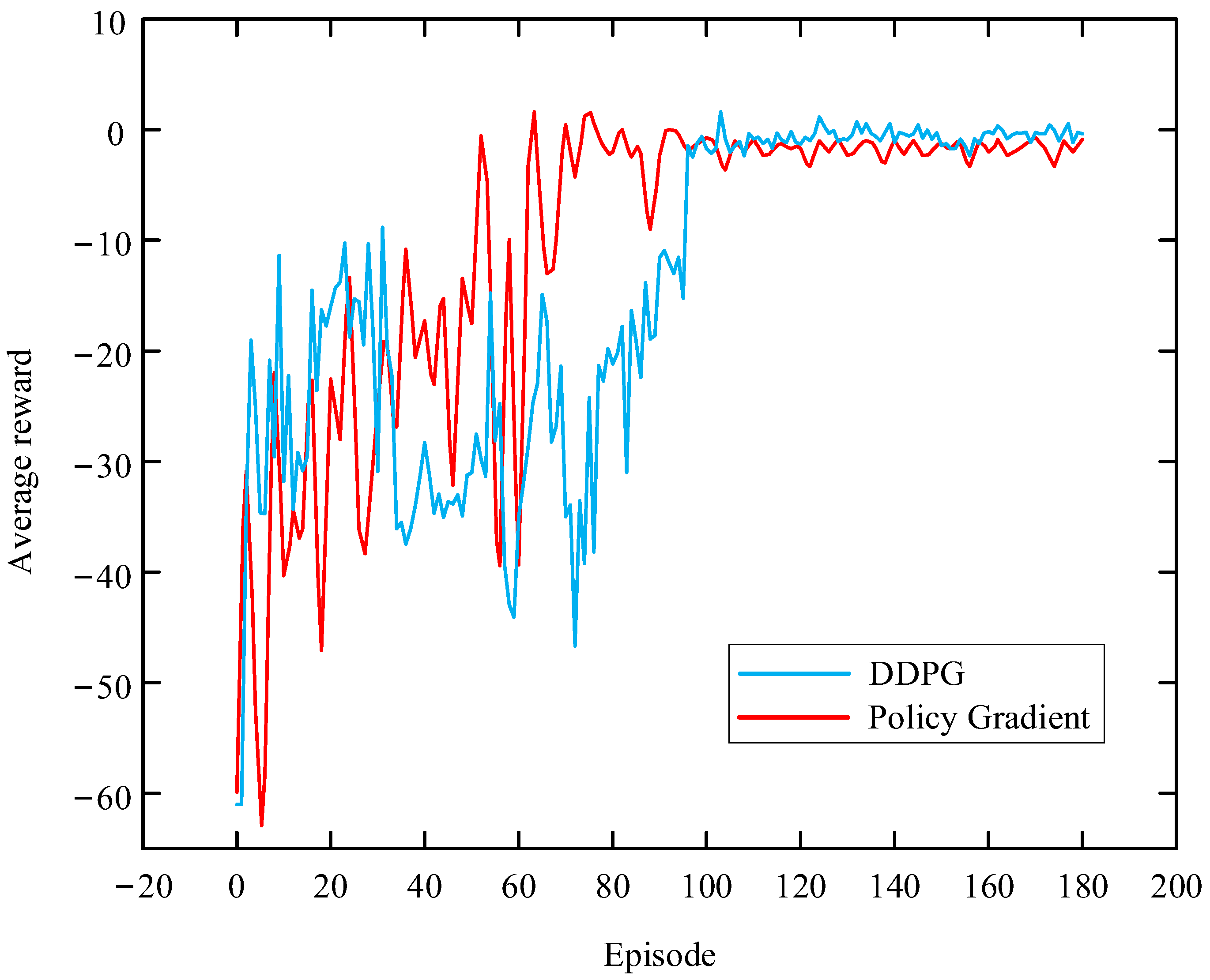
An automatic driving trajectory-planning method based on time series bird’s-eye view and policy gradient algorithm is designed. The policy gradient algorithm is used to improve the ability of automatic driving vehicle trajectory planning and the efficiency of Lattice sampling method for trajectory planning. The time series bird’s-eye view combined with the policy gradient algorithm can enhance the ability of feature extraction of the policy network, make the network convergence easier, and improve the feasibility of the method.
- (2)
The variable Gauss security field is added as the evaluation index of the reward function and control part to improve the security of trajectory and control effect.
2. Route Planning Algorithm
The goal of trajectory planning for autonomous driving is to find the optimal trajectory in advance for a vehicle. On the one hand, it is necessary to ensure the safety of the vehicle; On the other hand, getting to the destination through obstacles as soon as possible, reducing traffic pressure and improving driving efficiency are also important criteria to measure the effectiveness of the planned trajectory.
Figure 1 shows that the trajectory planning module plays a key role in the overall auto-driving system.
2.1. Time Series Bird’s-Eye View and Strategic Network
The agents of reinforcement learning obtain the state input through interaction with the surrounding complex traffic environment to conduct effective learning training. One of the difficulties of the existing reinforcement learning algorithm is obtaining effective state features from complex environments. Overly redundant states will increase the learning difficulty of the agent. It is particularly important to make it easier for an agent to extract valid features. Therefore, this paper designs a policy network and corresponding time series bird’s-eye view as the state quantity of the reinforcement learning, enabling the network to extract better environmental features.
2.1.1. Policy Network State Quantity
For an effective policy network for reinforcement learning, it is essential to obtain the perceptual information including lane lines, pedestrians, vehicles, and obstacles from the surrounding environment as well as the predictive tracks for the next few moments including dynamic obstacles.
The sequential bird’s-eye view significantly improves the learning efficiency of the policy network.
Figure 2 shows the time series bird’s-eye view matrix diagram.
The bird’s-eye view is a three-dimensional matrix composed of lateral displacement, vertical displacement and time. The specific elements in the matrix diagram shown in
Figure 2 include (a) the current position status of the ego vehicle, (b) the ego vehicle, (c) obstacles, (d) the non-driving area and (e) the exercisable area, (f) the reference line, (g) the planned trajectory.
The generation of the time series bird’s-eye view includes the following two steps: (1) According to the perception module of the autonomous vehicle, obtain the surrounding environmental information, including dynamic and static obstacles and lane lines. The prediction module is used to obtain the position information of dynamic obstacles in the future time of . (2) The information obtained from the perception module and the information is used to generate a bird’s-eye view of features in three dimensions: horizontal, vertical and time.
The size of the three-dimensional the time series bird’s-eye view matrix is (40, 400, 80). The first dimension 40 represents the horizontal range of 10 m on the left and right of the reference line, with the horizontal displacement interval of 0.5 m; The second dimension 400 represents the longitudinal 200 m forward range with the ego vehicle as the origin, the longitudinal displacement interval is 0.5 m, and the third dimension 80 represents the time range within the next 8 s, the time interval is 1 s. The (c) obstacles and (d) the non-driving area are represented by −1 in the time series bird’s-eye view matrix; (e) the exercisable area is represented by 0 in the time series bird’s-eye view matrix; (f) the reference line is represented by 1 in the time series bird’s-eye view. In the matrix, the reference line represents higher priority than (c) obstacles, (d) the non-driving area and (e) the exercisable area. At the same time, (a) the current position status of the ego vehicle, (b) the ego vehicle, and (g) the planned trajectory are not specifically represented in the time series bird’s-eye view matrix.
Figure 3 shows the vertical view of a time series bird’s-eye view with a green rectangle representing the vehicles on the highway and a dashed grey line representing the driveway sidelines.
The generation of a time series bird’s-eye view includes the following two steps: (1) Obtain the surrounding environment information, including dynamic and static obstacles, and lane lines, according to the perception module of the automobile. Obtain dynamic obstacles using prediction module in the future location information within the end. (2) Generate cross-sectional, vertical, and temporal feature bird’s-eye views using the information obtained from the perception and prediction modules. Then, train using the bird’s-eye view as the state input.
2.1.2. Strategic Network Structure
Figure 4 shows the structure of the policy network
. The network includes a convolution feature extraction network consisting of one convolution layer and a fully connected network consisting of three fully connected layers. Where
is the input state quantity of the policy network, including the time series bird’s-eye view matrix and the history track of the vehicle,
denote the weights and offset parameters for the network and
is the output of the policy network, that is, the final state of the planning trajectory
, where
,
and
are the final longitudinal position, the end-of-longitudinal speed, and the acceleration of the longitudinal end state of the vehicle, respectively, while
,
and
are the lateral end state position, the lateral end-state speed and the acceleration of the lateral end state of the vehicle, respectively. The input of the convolution feature extraction network is the time series aerial view matrix and the output is the final extracted environmental feature information. The input of the fully connected network is the convolution feature. The environmental feature information and the historical track information of the vehicle are extracted from the network output.
2.2. Variable Gauss Safety Field Theory
Since reinforcement learning explores policies and rewards by making agents constantly try and error, the security of reinforcement learning is lower than the other methods. Improving the security of reinforcement learning remains the focus of research. The variable Gauss security field model based on risk center transfer further improves the security of trajectory planning and control methods and serves as the reward function of the trajectory planning part and the constraint boundary of the control part.
Figure 5 shows that a static vehicle is abstracted as a rectangle with a length of
, a width of
, and the risk center
is its geometric center. The static security field of the vehicle is described by a two-dimensional Gaussian function as:
where
is the field strength factor,
and
represent the function of vehicle shape. The main control parameter for the shape of a static safety field is anisotropy:
Parameter equivalently expressed in aspect ratio .
The direction of the safety field is a vector from the risk center whose isoelectric line is projected upward into a series of ellipses. In
Figure 5, the red rectangle represents the vehicle, the area in the solid red rectangle is called the core domain, the area between the red and the yellow ellipses is called the restriction domain, the area between the yellow and the blue ellipses is called the expansion domain, and each area represents a different risk state. The sizes of these different domains are related to the shape and motion of the vehicle and can be determined based on the parameters
,
of the Gaussian function (1). The Gauss security field is variable. The aspect ratio of the virtual vehicle will change with the change of the vehicle motion state and will significantly change the core, restriction and extension domains of the Gauss security field.
Figure 6 shows the overhead projection of the dynamic safety field. It can be seen that when the vehicle is in motion, the risk center will transfer following the vector
, the new risk center becomes
and there are:
where
is the velocity vector of the vehicle motion,
is the regulator and
or
, the sign corresponds to the front and back directions of the movement.
is the transferred angle between the vector and the x-axis.
A virtual vehicle is formed with a length of
and width of
under the transfer of the risk center, whose geometric center is
, which establishes its dynamic security field as:
where
and
are parameters related to vehicle shape and motion state. The new aspect ratio is expressed as
.
2.3. Improved Lattice Programming Algorithm Based on Strategic Gradient Algorithm
The traditional Lattice programming algorithm achieves trajectory planning by sampling the target vertically and horizontally. This method will lead to the dilemma of a suboptimal solution for the sample-fitting trajectory, and it would be difficult to obtain the optimal trajectory. However, too many sampling points will lead to complex and inefficient calculations.
The Lattice algorithm is improved by using the policy gradient algorithm to directly obtain the optimal final state sample points as shown in
Figure 7. This improved method abandons sampling with high time complexity and cost function evaluation for each alternate trajectory, which considerably improves the timeliness of the algorithm. Although the training process of reinforcement learning has better universality than the general rule-based planning algorithm, the design of the reward function based on the final control effect will make it more suitable for complex traffic scenes and complex vehicle dynamic features.
2.3.1. Track Planning Agent Design
The trajectory output by general dynamic programming, Monte Carlo sampling and time series difference methods will have a complete state action sequence
and a trajectory consists of several state–action pairs as shown in
Figure 8. Different actions
in each step will inevitably lead to changes in the overall trajectory. This will necessarily result in an exponential increase in the complexity of the solution as the length of the trajectory will increase. The simplified trajectory
is composed of the start state
, action
and end state
. In the start state
, executing action
produces a unique trajectory
, reaching the end state
.
In practice, the policy gradient algorithm is used instead of the last state sampling process in the Lattice algorithm. The end state of the track is used as the action space
:
Policy network
maximizes the expected return of the output trajectory as an optimization objective:
where
denotes the state features of the surrounding traffic environment, a is the network output action,
is a network parameter,
is the probability of executing action a and outputting track
under parameter
and state
, and
is the reward function of trajectory
.
The gradient rise method is used to optimize
from Equation (6):
To calculate the derivative of the optimization objective with respect to network parameter
, the strategy gradient is derived as:
To improve the efficiency of training, during the training process, the agent continuously stores the experience data
from the interaction with the environment in real-time into the experience pool (Memory). The Monte Carlo method is also used to randomly extract the mini-batch-sized empirical data from the experience pool for training:
From Formula (9), the update direction of the final policy parameters
is:
To enhance the agent’s exploring ability in unfamiliar state space and avoid the agent falling into local optimal space during training, the output of the policy network
will conform to normal distribution. It consists of two parts: mean
and variance
:
During the learning process of the policy network , the mean and the variance of the output keep approaching and 0, respectively, and the probability of the agent taking random behavior exploration keeps decreasing. During training, the agent selects action from this normal distribution as the training output and executes it.
2.3.2. Reward Function Design
Reinforcement learning obtains the amount of state by interacting with the environment and evaluates the training agent by a reward function. The agents obtain higher returns by continuously optimizing their network of policies. Therefore, the design of the reward function is critical to the convergence of the agent, which affects the final decision-making results of the overall model. Moreover, a reasonable reward function design can also make the agent obtain more incentives from the environment and accelerate the convergence speed of the agent.
The reward function design for the trajectory planning section includes the following sections:
In the formula,
is the speed reward, its goal is to keep the speed at the target speed;
and
are the longitudinal and lateral comfort rewards, respectively, their goals are to maintain low longitudinal acceleration and low lateral acceleration, respectively;
is the lateral deviation reward, its goal is to maintain a small lateral deviation from the reference line;
is the additional coupling reward, the objective is to maintain the coupling force between the planned trajectory and the controller and vehicle dynamics, and to maintain a better horizontal and vertical tracking accuracy of the vehicle during actual tracking; and
is the safety reward.
is the proportion weight of each reward function. Where,
,
,
,
,
, and
. The value of
is obtained through debugging, and the specific value comparison is shown in
Figure 9 below.
The design of is constrained by the variable Gaussian safety field, as shown below:
When the vehicle is stationary:
When the vehicle is moving:
where
,
and
are the length and the width of the agent, respectively,
is the speed vector of vehicle motion,
is the adjustment factor, and
is the angle between the transfer vector and the x-axis. After the actual vehicle test,
= 0.35.
3. Controller Design
The traditional trajectory planning module and the control module are simple upper and lower-level relationships. The trajectory planning module outputs the optimal trajectory and the controller tracks the control. Although this mode is simple and easy to operate, it cannot meet the real-time requirements in complex traffic environments.
Figure 10 shows the relationship diagram of the proposed feedback design model. It can be seen from the figure that the trajectory planning agent based on the policy gradient algorithm, the trajectory tracking controller and the environment form a planning control environment closed loop. The proposed loop feedback design model will enable the agents to continuously learn to adapt to the environment and adapt to the trajectory tracking controller. This method effectively links the traffic environment, the planner and the controller, so that the output trajectory of the planner can effectively adapt to the dynamic features of the vehicle and the controller. To enable the agent to stably, efficiently and safely track the optimal trajectory output by the planner, and improve the efficiency, the training of the control part is divided into horizontal control and vertical control.
3.1. Horizontal Trajectory Tracking Control Model Training
The goal of the traditional horizontal trajectory tracking task [
19,
20] is to enable vehicles to drive stably on the lane line without deviating, regardless of the state relationship with other vehicles. However, when the vehicle tracks and controls the track, the first consideration is the safety of the track, that is, it will not collide with other vehicles. Therefore, the variable Gaussian safety field is introduced as the evaluation index, and the state quantity and reward function are adjusted. The variables including the distance
from other vehicles, the lateral relative coordinate
, the coordinate
of the navigation point in the current vehicle coordinate system, the heading deviation
and the speed
and acceleration
of the control vehicle are added as the state variables:
The output action is only the steering wheel angle
. For the design of the reward function for lane keeping, the lateral error
between the current vehicle coordinate and the lane centerline, the deviation
of the heading angle and the relative distance
from other vehicles are considered as the evaluation index reward functions:
where
,
and
are the length and the width of the agent, respectively,
is the speed vector of vehicle motion,
is the adjustment factor, and
is the angle between the transfer vector and the x-axis. After the actual vehicle test,
= 0.35.
If the lateral deviation of the current position of the autonomous vehicle is greater than the set maximum lateral deviation threshold value during the training, the current round of iterative training will be ended for the next round of training. Through the cumulative reward mechanism, agents that enhance learning continuously obtain higher reward reports. Hence, they can take more potential threats into account. However, the dynamic features of the vehicle will be hidden in the state quantity of the past few moments. Thus, it would be difficult to fully understand the current state of the intelligent vehicle only through the current state quantity. To enable the agent to better understand the dynamic features of the intelligent vehicle at the current time and output more reasonable trajectory tracking actions, the state quantities at the current time and at the past four times are stacked together as network inputs.
3.2. Training of Longitudinal Trajectory Tracking Control Model
To maintain an ideal distance between the ego vehicle and the vehicle in front without any collision with the vehicle in front, the ego vehicle is expected to cruise at a constant speed when there is no vehicle in front. When there are other vehicles in front of the ego vehicle, the road information is not considered, instead only the information of the current vehicle and the vehicle ahead is considered as the state quantity.
Figure 11 describes the cruise mission status. The longitudinal trajectory tracking control task considers the speed
and acceleration
of the current vehicle, speed
and acceleration
of the vehicle in front, the distance
from the vehicle in front and the expected speed
of the current vehicle as the state variables:
Output action
of the agent, including accelerator action
and brake action
:
For vertical control tasks, the reward function is designed as:
where
and
are the expected and safe distances from the vehicle in front, respectively. When the distance between the intelligent vehicle and the vehicle in front is less than the safe distance, the reward is −100 and the current interaction is stopped to start the next round of interaction. During longitudinal training, the speed
of the vehicle in front and the expected speed
of the current vehicle are randomly given each round, so that the training model can be generalized to more complex situations.
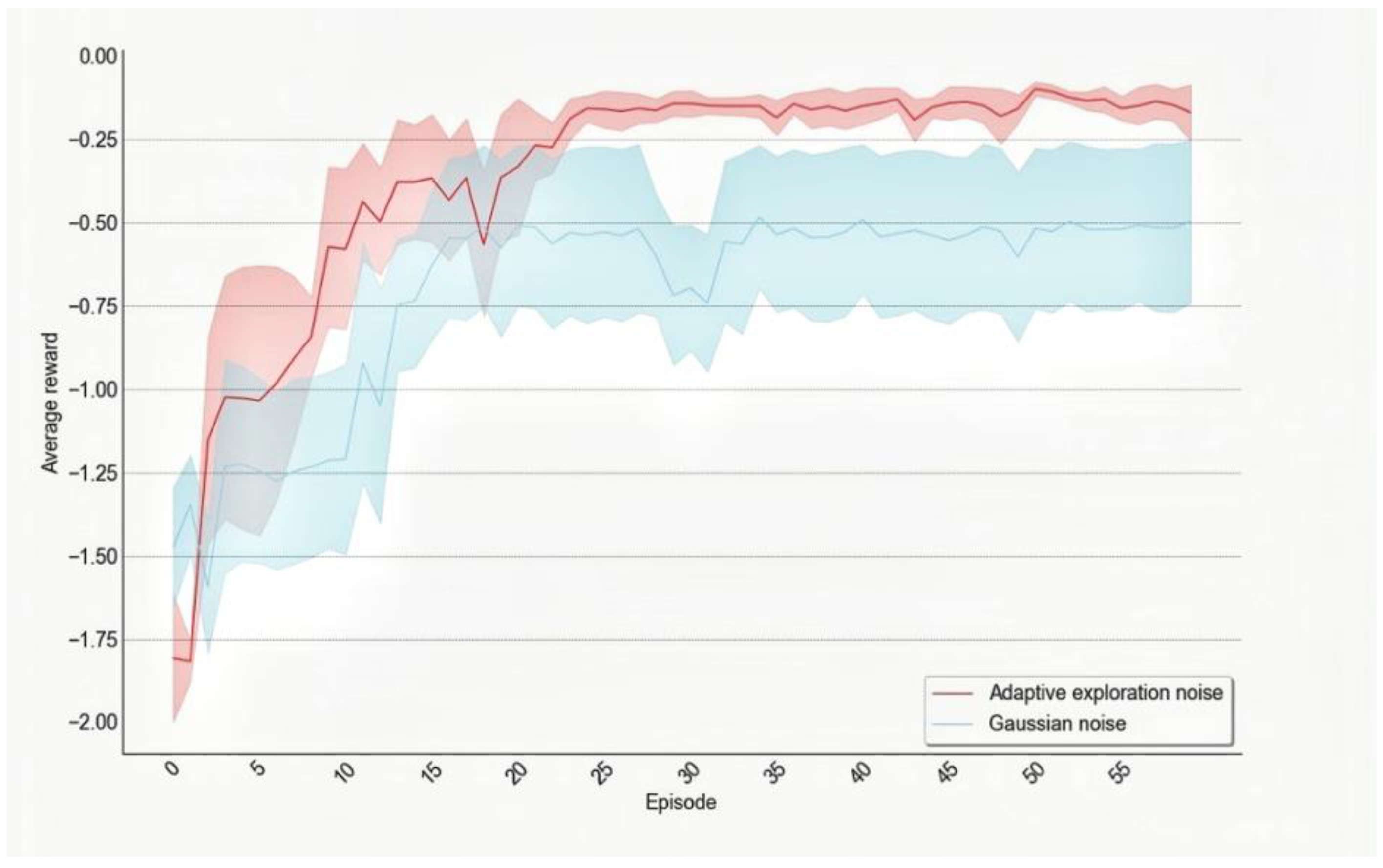
The traditional training mostly uses Gaussian noise or Ornstein Uhlenbeck (OU) noise to promote agents to actively explore the environment at the beginning of training. However, unnecessary exploration will prolong the training time of agents. Therefore, in this paper, a Multi-Head Actor network structure is designed for the tasks with convex solution space in longitudinal control tasks. The main function of the proposed structure is to make the output action noisy. Action noise reflects the uncertainty measure of the optimal solution of the current policy. The Multi-head Actor network structure is used to construct this uncertainty measurement method.
The output of the Online Actor network is connected to multiple Head networks. To reflect the difference of each Head network, the initialization and training sampling experience pool of each Head network are independent and the way to converge to the optimal solution space is also different. Therefore, the variance of the Head network output action is used to estimate the uncertainty measure of the output action of the Actor network as:
where
and
are the real-time action noise and the threshold noise, respectively,
is the adopted policy,
is the deterministic action of the network output, and
is the weight parameter.
Similar to the horizontal control part, the vertical control part also selects the current state quantity of the agent and the state quantity of the past four times as the network input, making the network easier to converge and having high training efficiency.
5. Conclusions
In this paper, a vehicle safety planning control method based on the variable Gaussian safety field is designed. The policy gradient algorithm is used to improve the driving safety of autonomous vehicles and make the driving trajectory of autonomous vehicles more intelligent. The spatiotemporal bird’s-eye view proposed in combination with the policy gradient algorithm as a state variable can enhance the ability of feature extraction of the policy network and make the network convergence easier. The variable Gaussian safety field is added as the reward function of the trajectory planning module and the evaluation index of the control module to improve the safety and rationality of the output trajectory and tracking control, respectively. In the longitudinal control module, Gaussian noise input is improved to avoid repeated invalid exploration of agents and enhance training efficiency. Compared with the traditional planning control algorithm, the proposed method has the following advantages: (1) the spatiotemporal bird’s-eye view is used as the input state of the policy network enabling the trajectory planning policy network to effectively extract the features of the surrounding traffic environment. The planning trajectory of autonomous vehicles is generated through reinforcement learning, which improves the trajectory planning ability of autonomous vehicles in complex scenes. The efficiency of the lattice sampling method for trajectory planning algorithm avoids invalid sampling in complex traffic scenes; (2) the variable Gaussian safety field is added as a reward function to improve the safety of trajectory and control effect; (3) the traditional noise input is improved and the multi-head actor network structure is designed to add noise in the output action and improve the training efficiency. The experimental results demonstrate and validate that the proposed framework is superior to the traditional methods.
At the same time, this paper does not consider the scenarios other than an expressway, and how to change lanes in an emergency. In the future, we will test and improve the algorithm in more complex environments, such as ramps and urban roads. From another point of view, the single vehicle will be extended to the fleet, and the driving efficiency and safety of the fleet on the expressway will be considered.


