VSI Nonlinearity Compensation of a PMSM Drive System Using Deadbeat Prediction Based Current Zero-Crossing Detection

Abstract

Due to the nonlinearities of the voltage-source inverter (VSI) in a permanent magnet synchronous machine (PMSM) drive system, there is always an error between the reference voltage and the actual output voltage. To compensate the voltage error, many schemes have been proposed based on the phase current polarity. However, due to factors such as current clamping, measurement noises, and control system delay, the accuracy of the detected current polarity is relatively low, especially when the current is around zero, which would therefore affect the compensation performance. To solve this issue, a deadbeat prediction-based current zero-crossing detection method (DP-CZD) is proposed in this paper. With the proposed method, the measured three-phase currents are replaced by the predicted three-phase currents in terms of the polarity determination, when the absolute value of the phase current is within the threshold range. Compared with the conventional phase current polarity detecting methods, the proposed method can greatly improve the accuracy of detected current polarity due to its smooth transient waveform, and consequently, contributes to the much higher accuracy and lower total harmonic distortion (THD) in the compensation of VSI nonlinearity, which is verified through a prototype surface-mounted PMSM.

1. Introduction

Due to its simple structure, high efficiency and high energy density, the permanent magnet synchronous machine (PMSM) drive system, which is usually fed by voltage-source inverters (VSIs), is widely applied in electric vehicles, wind turbines and industrial servo drives [1]. However, due to the VSI nonlinearities caused by the dead time, turn on/off delay and voltage drops of power devices, the output voltage of the inverter would be distorted, which would further cause the increase in current harmonics and deteriorate the control performance. In addition, the accuracies of some conventional control methods, such as parameter identification [2,3,4] and sensorless control [5,6,7,8,9,10,11], in which the reference voltage is utilized to replace the actual voltage, would be affected by the distorted voltage due to VSI nonlinearity [12].

To solve the problems caused by the voltage error, many methods have been proposed. In Refs. [13,14], the hardware-based method is proposed to eliminate the dead time, by decomposing the universal phase leg into two basic switching units and designing a complex programmable logic device, which can realize the inverter operation without dead time. However, additional hardware circuits are required to detect the direction of the phase current, and the turn-on/off delays of the switches are still not considered in [13,14]. Comparatively, compensating the VSI nonlinearity from the perspective of the control algorithm is more attractive, considering its practicality. According to the existing literature, the compensating methods for VSI nonlinearity can be mainly divided into the following four groups:

(1)

Harmonic analysis methods. A low pass filter is used to separate high-frequency harmonic components of the control system. Then, the distortion voltage is estimated by minimizing the harmonics. Finally, the disturbance voltage due to the VSI nonlinearity is suppressed by performing feedback compensation [4,15,16,17,18,19];

(2)

State variable estimation. Additional feedback is constructed by selected state variables, nominal parameters of machines and VSI. Then, the distortion voltage using state variables is estimated and compensated for to make the trajectory of the voltage vector more circular [12,20,21,22,23,24].

(3)

Model predictive control. The relationship between the voltage sector and current polarity are modeled and the error of the voltage vector can be obtained by the polarity of the current and real-time switching state. Finally, the synthesized voltage vectors can be applied to PWM-VSI to enhance the system’s performance [25,26,27].

(4)

Repetitive controller. It is assumed in Refs. [28,29] that the disturbance signal of the previous fundamental period is repeated at the same instant of the next period. On this basis, the controller generates an appropriate output according to the difference between the given and feedback signals, which can reduce the voltage distortion and improve the robustness of the system.

Compared with other methods, the harmonic analysis method is more attractive for its convenient and easy application in the digital controller. However, due to factors such as current clamping, current measurement noise and control system delay, the accuracy of the detected current polarity around the zero-crossing is seriously affected, which would deteriorate the performance of compensation.

To solve this issue, a VSI nonlinearity compensation method using deadbeat prediction-based current zero-crossing detection (DP-CZD) is proposed in this paper. First, the time delay caused by the updating mechanism of the microprocessor is analyzed, in terms of the space vector pulse width modulation (SVPWM) implementation [30]. Then, the predicted currents in the dq–axis are predicted according to the current predictive model and further used to calculate the predictive voltages, thus mitigating the time delay through the compensation of one-step delay. Furthermore, the predicted three-phase currents, which can be obtained from the predicted currents in the dq-axis through Park transformations, are constantly compared with the actual phase currents. Once the actual phase currents are within the pre-defined threshold value during the zero-crossing process, the polarity of the predicted currents, instead of the conventional actual phase currents, is applied for the determination of output voltage. This innovation would greatly improve the compensation accuracy of the VSI nonlinearity, as the predicted three-phase currents have no clamping phenomenon and can smoothly cross the zero point. Finally, the proposed method is tested in a prototype surface-mounted PMSM system.

With the proposed method, the voltage error between the reference and the actual output can be minimized, which can be applied to improve the technique through which the reference voltage is directly used to replace the actual output voltage, such as the conventional sensorless method and parameter identification.

The organization of this paper is as follows. In Section 2, the voltage model considering the VSI’s nonlinearity is established. In Section 3, the VSI nonlinearity compensation method using direct measurement-based current zero-crossing detection (DM-CZD) is developed. In Section 4, the proposed VSI nonlinearity compensation method based on DP-CZD is given and the effects of parameter mismatches on DP-CZD are analyzed. The performance of the proposed VSI nonlinearity compensation method is experimentally tested in Section 5. Finally, conclusions are drawn in Section 6.

2. Mathematical Model of PMSM System Considering the VSI Nonlinearity

Assuming that the copper loss, iron loss, and back electromotive force (EMF) harmonics of PMSM can be neglected, the steady-state of the dq-axis voltages Equations in SPMSM [2] can be expressed as

$$\left[\begin{array}{c}{u}_d\left(k\right)\\ u_q\left(k\right)\end{array}\right]=\left[\begin{array}{cc}R& -L_s{\omega }_e\left(k\right)\\ L_s{\omega }_e\left(k\right)& R\end{array}\right]\left[\begin{array}{c}{i}_d\left(k\right)\\ i_q\left(k\right)\end{array}\right]+\left[\begin{array}{c}0\\ {\psi }_f{\omega }_e\left(k\right)\end{array}\right]$$

(1)

where k represents the index of the sampling moment in the discrete state, and $u_d$ and $u_q$ are actual voltages. The model of dq-axis voltage Equations considering the VSI nonlinearity [3] can be expressed as:

$$\left[\begin{array}{c}{u}_{{}_d}^{*}\left(k\right)\\ u_{{}_q}^{*}\left(k\right)\end{array}\right]+\left[\begin{array}{c}\mathit{Dd}\left(k\right)V_{\mathit{dead}}\\ \mathit{Dq}\left(k\right)V_{\mathit{dead}}\end{array}\right]=\left[\begin{array}{cc}R& -L_s{\omega }_e\left(k\right)\\ L_s{\omega }_e\left(k\right)& R\end{array}\right]\left[\begin{array}{c}{i}_d\left(k\right)\\ i_q\left(k\right)\end{array}\right]+\left[\begin{array}{c}0\\ {\psi }_f{\omega }_e\left(k\right)\end{array}\right]$$

(2)

where $u_d^{*}$ and $u_q^{*}$ are the reference dq-axis voltages, Dd(k)V_dead and Dq(k)V_dead are distorted voltages caused by VSI nonlinearity, and V_dead can be seen as constant under the steady state and can be expressed as [9]:

$$V_{\mathit{dead}}=\frac{T_{\mathit{dead}}+T_{\mathit{on}}-T_{\mathit{off}}}{3T_s}\left(V_{\mathit{dc}}-V_{\mathit{sat}}+V_d\right)+\frac{V_{\mathit{sat}}+V_d}{6}$$

(3)

In Equation (3), V_dead is the distorted voltage due to inverter nonlinearity, T_s and T_dead represent the sampling interval and dead time, respectively, T_on and T_off are the turn-on/off delay of IGBT, and V_dc, V_sat and V_d represent DC bus voltage, the forward voltage drops of the switching tube and the freewheeling diode, respectively.

The three-phase voltage distortions $V_{\mathit{as}}^{\mathit{err}}$, $V_{\mathit{bs}}^{\mathit{err}}$ and $V_{\mathit{cs}}^{\mathit{err}}$ due to VSI nonlinearity can be expressed as follows [15]:

$$V_{as}^{err}=\left(2\mathrm{sign}\left(i_a\right)-\mathrm{sign}\left(i_b\right)-\mathrm{sign}\left(i_c\right)\right)V_{\mathit{dead}}+\frac{r_{ce}+r_d}{2}{i}_a$$

$$V_{bs}^{err}=\left(2\mathrm{sign}\left(i_b\right)-\mathrm{sign}\left(i_a\right)-\mathrm{sign}\left(i_c\right)\right)V_{\mathit{dead}}+\frac{r_{ce}+r_d}{2}{i}_b$$

$$V_{cs}^{err}=\left(2\mathrm{sign}\left(i_c\right)-\mathrm{sign}\left(i_a\right)-\mathrm{sign}\left(i_b\right)\right)V_{\mathit{dead}}+\frac{r_{ce}+r_d}{2}{i}_c$$

$$\mathrm{sign}\left(i\right)=\left\{\begin{array}{l}1,i\ge 0\\ -1,i<0\end{array}\right.$$

(4)

where r_ce and r_d are the on-resistance of the switching tube and freewheeling diode; after the Park transformation, the distorted voltages $V_d^{\mathit{err}}$ and $V_q^{\mathit{err}}$ in the dq-axis reference frame could be written as [15]:

$$\left[\begin{array}{c}{V}_d^{err}\\ V_q^{err}\end{array}\right]=\left[\begin{array}{c}Dd{V}_{dead}\\ Dq{V}_{dead}\end{array}\right]=\frac{2}{3}\left[\begin{array}{ccc}\cos \left(\theta \right)\hfill & \cos \left(\theta -\frac{2\pi }{3}\right)& \hfill \cos \left(\theta +\frac{2\pi }{3}\right)\\ -\sin \left(\theta \right)\hfill & -\sin \left(\theta -\frac{2\pi }{3}\right)& \hfill \sin \left(\theta -\frac{\pi }{3}\right)\end{array}\right]\left[\begin{array}{c}{V}_{as}^{err}\\ V_{bs}^{err}\\ V_{cs}^{err}\end{array}\right]$$

Thus, Dd and Dq can be expressed as:

$$\left[\begin{array}{c}\mathit{Dd}\\ \mathit{Dq}\end{array}\right]=2\left[\begin{array}{ccc}\cos \left(\theta \right)\hfill & \cos \left(\theta -\frac{2\pi }{3}\right)& \hfill \cos \left(\theta +\frac{2\pi }{3}\right)\\ -\sin \left(\theta \right)\hfill & -\sin \left(\theta -\frac{2\pi }{3}\right)& \hfill \sin \left(\theta -\frac{\pi }{3}\right)\end{array}\right]\left[\begin{array}{c}\mathrm{sign}\left(i_a\right)\\ \mathrm{sign}\left(i_b\right)\\ \mathrm{sign}\left(i_c\right)\end{array}\right]$$

(5)

As detailed in Refs. [15,21], if γ represents the angle between current vector and q-axis, and θ_e = θ + π/2, the distorted voltages caused by VSI nonlinearity vary in different cases and are be shown in

Table 1. Relationship of phase current polarities and dq-axis distorted voltage.

Case	θe	Sign(i)			VdeadDd	VdeadDq
		ia	ib	ic
1	−π/6 – λ ~ π/6 − λ	1	−1	−1	4Vdeadsin(θe)	4Vdeadcos(θe)
2	π/6 − λ ~ π/2 − λ	1	1	−1	4Vdeadsin(θe − π/3)	4Vdeadcos(θe − π/3)
3	π/2 – λ ~ 5π/6 − λ	−1	1	−1	4Vdeadsin(θe − 2π/3)	4Vdeadcos(θe − 2π/3)
4	5π/6 − λ ~ 7π/6 − λ	−1	1	1	4Vdeadsin(θe − π)	4Vdeadcos(θe − π)
5	7π/6 – λ ~ 3π/2 − λ	−1	−1	1	4Vdeadsin(θe − 4π/3)	4Vdeadcos(θe − 4π/3)
6	3π/2 − λ ~ 11π/6 − λ	1	−1	1	4Vdeadsin(θe − 5π/3)	4Vdeadcos(θe − 5π/3)

.

In Figure 1a, the simulated waveforms of Dd and Dq obtained by Equations (4) and (5) are shown, under the electrical period of 0.1 s, from which it can be seen that distorted voltage in the d-axis is a zero-mean 6th harmonic component, and the q-axis voltage is composed of a DC and a 6th harmonic component. Consequently, the dq-axis currents also have a 6th harmonic component, as shown in Figure 1b.

3. Conventional Compensation Scheme of VSI Nonlinearity Using DM-CZD

The structure of the VSI nonlinearity compensation process using conventional DM-CZD can be shown in Figure 2, from which it can be seen that the compensation process can be divided into three parts, i.e., (1) V_dead estimation, (2) process of V_dead minimization, and (3) voltage feedback compensation.

From Equation (2) and Figure 2, the reference voltage of the d-axis $u_d^{*}$ can be obtained under the control of $i_d=0$ as:

$$u_d^{*}\left(k\right)=-\mathit{Dd}\left(k\right)V_{\mathit{dead}}-L_s{\omega }_e\left(k\right)i_q\left(k\right)$$

(6)

The 6th harmonic component Dd(k)V_dead accounts for the dominant component compared with other high-frequency harmonics in the d-axis voltage equation, and a method in Ref. [17] has been proposed to extract Dd(k)V_dead, which is shown in Figure 2b. The low-frequency and DC components of the voltage in the d-axis can be filtered through a low-pass filter to obtain the d-axis high-frequency voltage $u_{\mathit{dh}}^{*}\approx -\mathit{Dd}\left(k\right)V_{\mathit{dead}}$.

The Adaline neural network algorithm (Adaline NN) is simple and needs little CPU calculation. For example, it can be applied as an adaptive filter [31], which can smooth the estimated terms. Similarly, it can also be used to design the estimator of $V_{\mathit{dead}}$, as shown in Equation (7):

$${\hat{V}}_{\mathit{dead}}\left(k+1\right)={\hat{V}}_{\mathit{dead}}\left(k\right)+2\eta \mathit{Dd}\left(k\right)e\left(k\right)$$

(7)

where ${\hat{V}}_{\mathit{dead}}$ is the estimated distorted voltage, η is the convergence factor of the least mean square algorithm (LMS), Dd(k) is calculated from Equation (5), X_i = −Dd(k), W_i = ${\hat{V}}_{\mathit{dead}}$, $O=-\mathit{Dd}\left(k\right){\hat{V}}_{\mathit{dead}}$, $d\left(k\right)=u_{\mathit{dh}}^{*}\left(k\right)$, and $e\left(k\right)=u_{\mathit{dh}}^{*}\left(k\right)-O$.

The principles of the Adaline NN are detailed in Appendix A.

It can be seen from Figure 2 that the polarities of three-phase currents are required in the calculation of Dd and Dq in Equation (5). The phase A current fluctuates within ±0.1A during its zero-crossing in Figure 3a. The results of the VSI nonlinearity compensation utilizing DM-CZD are shown in Figure 3b,c, from which it can be seen that the distortion would occur when the phase current is near zero. Meanwhile, spikes are observed obviously in the dq-axis currents. When the three-phase currents are near zero, the calculated Dd and Dq values in Figure 3c tempestuously fluctuate, due to the influence of current clamping, current measurement noise and control system delay. Consequently, the VSI nonlinearity compensation is of low accuracy during the zero-crossing of three-phase currents, just as indicated in Figure 3b.

4. The Proposed Compensation Scheme of VSI Nonlinearity Using DP-CZD

4.1. DP-CZD and Compensation of VSI Nonlinearity

Considering the small sampling interval T_s, the angular velocity of the rotor can be seen as constant [30,32,33,34,35]. Consequently, the discrete model of the PMSM system can be given as Equation (9).

$$\left[\begin{array}{c}{u}_d\left(k\right)\\ u_q\left(k\right)\end{array}\right]=\left[\begin{array}{cc}R-\frac{L_s}{T_s}& -L_s{\omega }_e\left(k\right)\\ L_s{\omega }_e\left(k\right)& R-\frac{L_s}{T_s}\end{array}\right]\left[\begin{array}{c}{i}_d\left(k\right)\\ i_q\left(k\right)\end{array}\right]+\frac{L_s}{T_s}\left[\begin{array}{c}{i}_d\left(k+1\right)\\ i_q\left(k+1\right)\end{array}\right]+\left[\begin{array}{c}0\\ {\psi }_f{\omega }_e\left(k\right)\end{array}\right]$$

(8)

Due to the updating mechanism, there is always a time delay in the SVPWM implementation, as is shown in Figure 4 [30]. The relationship between the actual and reference voltages in dq-axis can be expressed as $u_{\mathit{dq}}\left(k\right)=u_{{}_{\mathit{dq}}}^{*}\left(k-1\right)$. When the reference voltages of the dq-axis $u_{{}_{\mathit{dq}}}^{*}\left(k\right)$ update, the actual dq-axis currents become $i_d\left(k+1\right)$ and $i_q\left(k+1\right)$, which would lead to inaccurate reference voltages. As such, the prediction of currents at the (k + 1) th instant is necessary to compensate this delay.

The predicted currents can be obtained from Equation (8) as:

$$\left\{\begin{array}{l}{\hat{i}}_d\left(k+1\right)=\left(1-R{T}_s/L_s\right)i_d\left(k\right)+T_s{\omega }_e{i}_q\left(k\right)+u_d\left(k\right)T_s/L_s\\ {\hat{i}}_q\left(k+1\right)=\left(1-R{T}_s/L_s\right)i_q\left(k\right)-T_s{\omega }_e{i}_d\left(k\right)+u_q\left(k\right)T_s/L_s-T_s{\omega }_e{\psi }_f/L_s\end{array}\right.$$

(9)

Electrical angular speed ω_e and electrical parameters are employed in Equation (8) for substituting the reference currents $i_d^{*}\left(k\right)$ and $i_q^{*}\left(k\right)$ into (8) at the k + 1th instant. Considering the time delay compensation, the estimated voltages can be consequently derived as:

$$\left[\begin{array}{c}{\hat{u}}_d\left(k\right)\\ {\hat{u}}_q\left(k\right)\end{array}\right]=\left[\begin{array}{cc}R-\frac{L_s}{T_s}& -L_s{\omega }_e\left(k\right)\\ L_s{\omega }_e\left(k\right)& R-\frac{L_s}{T_s}\end{array}\right]\left[\begin{array}{c}{\hat{i}}_d\left(k+1\right)\\ {\hat{i}}_q\left(k+1\right)\end{array}\right]+\frac{L_s}{T_s}\left[\begin{array}{c}{i}_d^{*}\left(k\right)\\ i_q^{*}\left(k\right)\end{array}\right]+\left[\begin{array}{c}0\\ {\psi }_f{\omega }_e\left(k\right)\end{array}\right]$$

(10)

From Equation (9), the predicted phase current can be obtained, which is shown in Figure 5. Compared with the measured phase current, the predicted current in Figure 5 can effectively track the measured one with no phase delay. In the partial zoomed-in part, the predicted phase current has no clamping phenomenon and smoothly crosses the zero point, while the measured phase current crosses the zero point repeatedly when it is near zero. Thus, the polarity of the measured three-phase currents can be replaced by the predicted three-phase currents to improve the accuracy of VSI nonlinearity compensation.

Conclusively, the main steps of the VSI nonlinearity compensation with the proposed DP−CZD method are as follows:

Step 1: Sampling the SPMSM rotor position, speed and phase currents;

Step 2: Calculating the predicted dq-axis currents with Equation (9), and obtaining the predicted three-phase currents i_pa, i_pb and i_pc by inverse Clark and Park transformations.

Step 3: Monitoring the measured three-phase currents. When the absolute values of the measured three-phase currents are less than the threshold i_thr, the polarity of the measured three-phase currents can be replaced by the predicted three-phase currents, which can finally be used to compensate VSI nonlinearity. The maximum fluctuation of the three-phase currents at the zero-crossing are considered in the current threshold i_thr, which are determined by specific working conditions.

The schematic diagram of VSI nonlinearity compensation with the proposed DP-CZD is shown in Figure 6 and Figure 7. In Figure 6, $u_d^{*}$ and $u_q^{*}$ are obtained by the proportional integral (PI) current loop regulator, while $u_d^{*}$ and $u_q^{*}$ in Figure 7 are calculated by the current predictive model. ${\hat{i}}_d\left(k\right)$ and ${\hat{i}}_q\left(k\right)$ are the predicted d-axis and q-axis currents, respectively. i_pa, i_pb and i_pc are the predicted three-phase currents. Furthermore, the distortion voltage V_dead, which is affected by rotor position, is estimated by Equation (7). Considering that the response of the control system is nonlinear, an online regulator is employed in this paper to adjust compensation voltages.

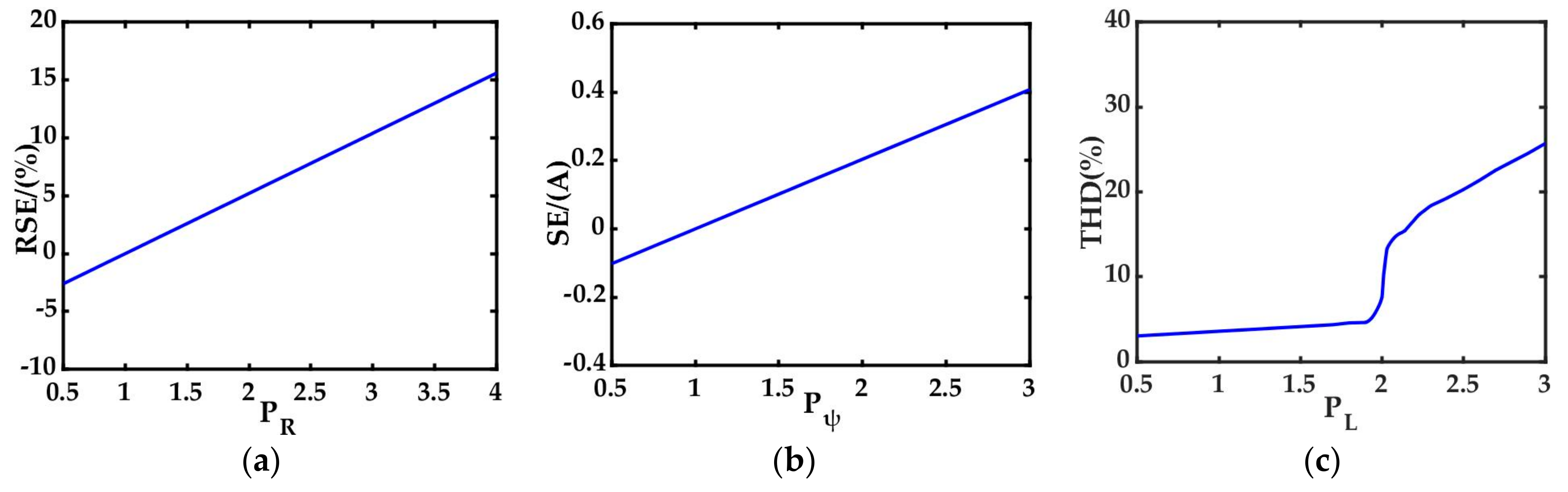
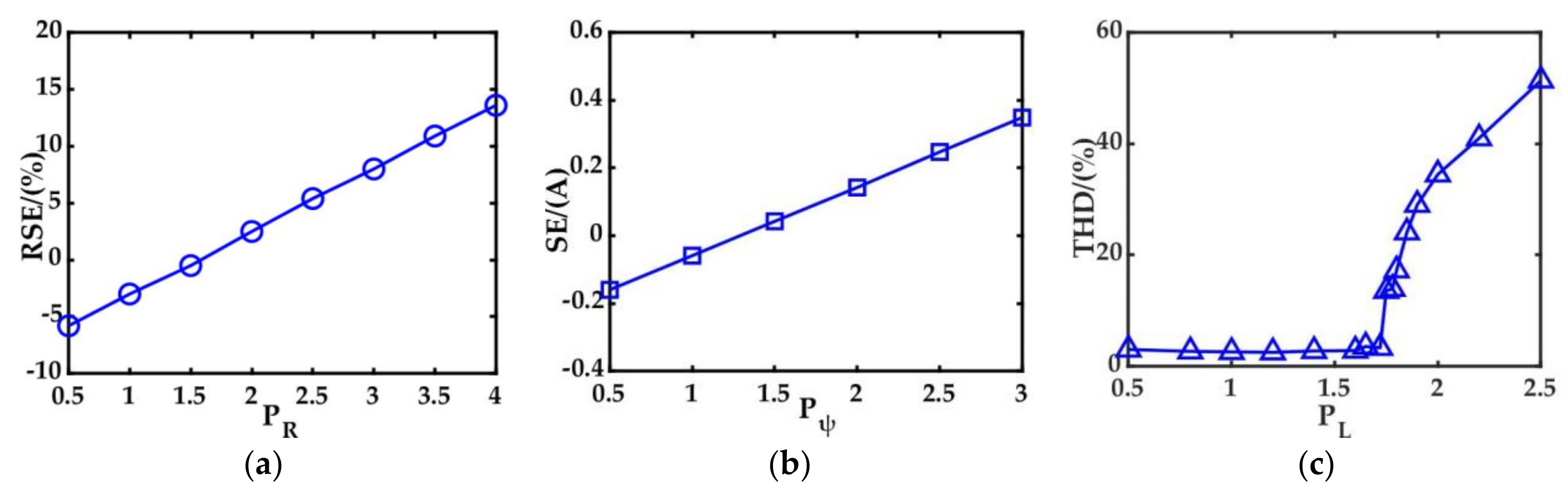
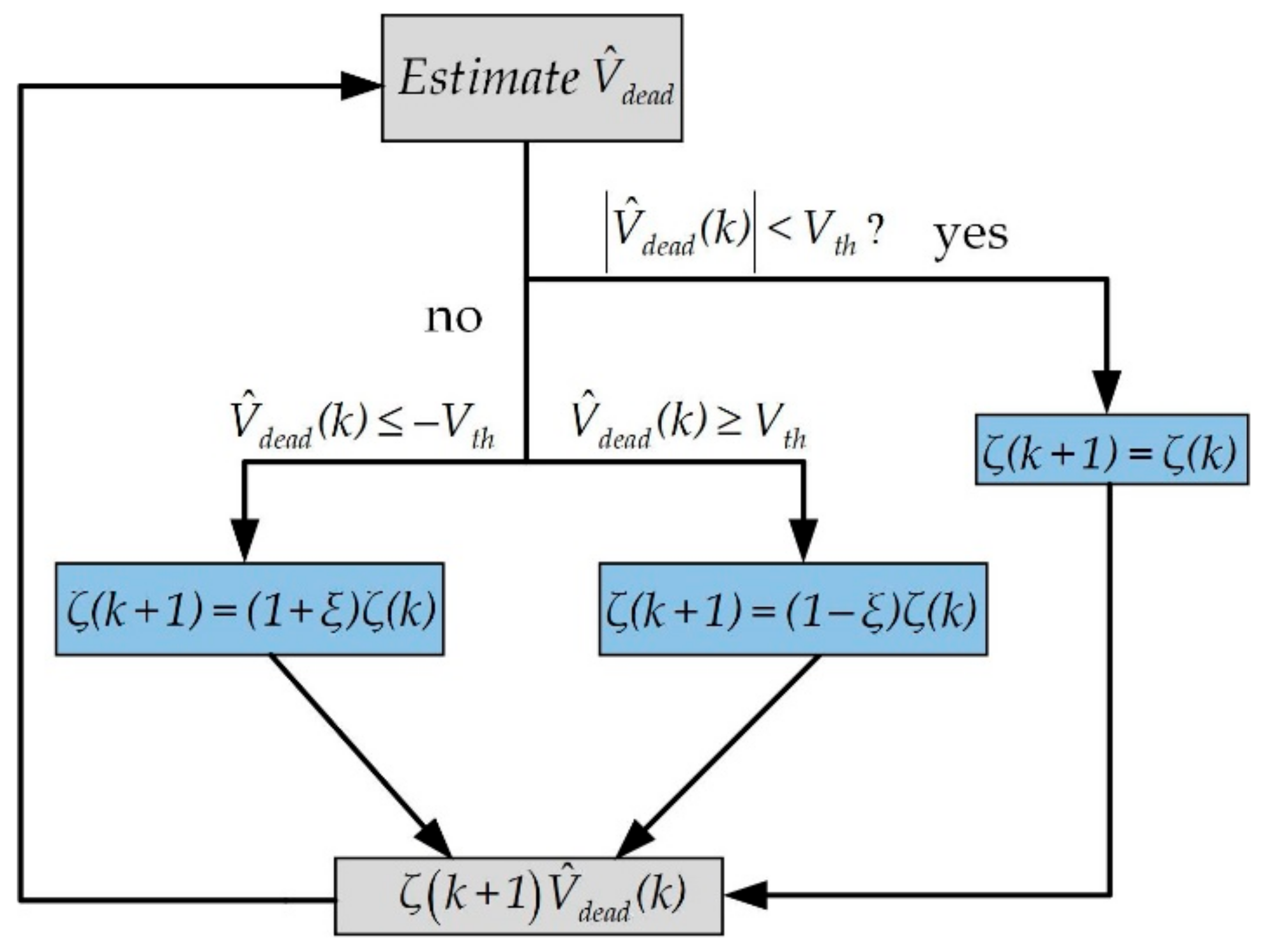
4.2. DP-CZD with Parameter Uncertainty

It can be seen from Equation (9) that current prediction is based on the parameters of the drive system, including sampling interval, electrical speed, stator winding resistance, stator inductance and permanent magnetic flux linkage [33,34,35]. Obviously, the mismatch of the above parameters would lead to the error in the current prediction. In this paper, the effects of parameters’ deviations involving stator winding resistance, stator inductance and permanent magnet flux linkage are analyzed. While the electrical speed ω_e and sampling interval T_s are kept the same in Equations (8–12, 15–17), the real currents at the k + 1 instant can be expressed as:

$$\left\{\begin{array}{c}{i}_d\left(k+1\right)=\left(1-R_r{T}_s/L_r\right)i_d\left(k\right)+T_s{\omega }_e{i}_q\left(k\right)+u_d\left(k\right)T_s/L_r\hfill \\ i_q\left(k+1\right)=\left(1-R_r{T}_s/L_r\right)i_q\left(k\right)-T_s{\omega }_e{i}_d\left(k\right)+u_q\left(k\right)T_s/L_r-T_s{\omega }_e{\psi }_r/L_r\hfill \end{array}\right.$$

(11)

Further, the relationship between feedback and predicted currents can be obtained by substituting Equation (9) into (11):

$$\left\{\begin{array}{c}{i}_d\left(k+1\right)=\frac{L_s}{L_r}{\hat{i}}_d\left(k+1\right)+\frac{T_s}{L_r}\left(R-R_r\right)i_d\left(k\right)+\left(1-\frac{L_s}{L_r}\right)i_d\left(k\right)+\left(1-\frac{L_s}{L_r}\right)T_s{\omega }_e{i}_q\left(k\right)\hfill \\ i_q\left(k+1\right)=\frac{L_s}{L_r}{\hat{i}}_q\left(k+1\right)+\frac{T_s}{L_r}\left(R-R_r\right)i_q\left(k\right)+\left(1-\frac{L_s}{L_r}\right)i_q\left(k\right)+\left(1-\frac{L_s}{L_r}\right)T_s{\omega }_e{i}_d\left(k\right)+\frac{T_s{\omega }_e}{L_r}\left({\psi }_f-{\psi }_r\right)\hfill \end{array}\right.$$

(12)

From the above Equations, it can be seen that the effects of mismatched permanent magnet flux linkage, stator winding resistance and stator inductance on current prediction are coupled. For better analysis, the influence of the above mismatched parameters is discussed in this section, respectively.

If only the mismatched stator winding resistance is considered, then Equation (12) can be simplified as:

$$\left\{\begin{array}{c}{i}_d\left(k+1\right)={\hat{i}}_d\left(k+1\right)+\frac{T_s}{L_r}\left(R-R_r\right)i_d\left(k\right)\hfill \\ i_q\left(k+1\right)={\hat{i}}_q\left(k+1\right)+\frac{T_s}{L_r}\left(R-R_r\right)i_q\left(k\right)\hfill \end{array}\right.$$

(13)

The ratio of R and R_r is defined as P_R, and then the relationship between feedback and predicted currents can be expressed as:

$$i\left(k+1\right)=\hat{i}\left(k+1\right)+\frac{T_s{R}_r}{L_r}\left(P_R-1\right)i\left(k\right)$$

(14)

Applying the z-transform to Equation (14), the scope of P_R can be defined as:

$$1-\frac{L_r}{T_s{R}_r}<P_R<1+\frac{L_r}{T_s{R}_r}$$

Usually, T_SR_r is much smaller than L_r. So, the effect of R on stability is almost negligible. However, mismatched stator winding resistance would cause a steady state error between predicted and actual currents. The relative steady error (RSE) can be defined as $\left(i-\hat{i}\right)/i$.

Figure 8 shows the simulation results of the relationship between current prediction errors and parameter mismatches. If only permanent magnet flux linkage mismatch is taken into account, then the q-axis current in Equation (12) can be simplified as:

$$i_q\left(k+1\right)={\hat{i}}_q\left(k+1\right)+\frac{T_s{\omega }_e}{L_r}\left({\psi }_f-{\psi }_r\right)$$

(15)

The ratio of ψ_f and ψ_r is defined as P_ψ, and relationship between feedback and predicted q-axis currents in Equation (16) can be expressed as:

$$i_q\left(k+1\right)={\hat{i}}_q\left(k+1\right)+\frac{T_s{\omega }_e{\psi }_r}{L_r}\left(P_{\psi }-1\right)$$

(16)

As shown in Equation (16), mismatched permanent magnet flux linkage has no effect on the stability of the control system. However, the steady state error (SE) still exists, which is shown in Figure 8b.

If only stator inductance mismatch is considered, then Equation (12) can be expressed as:

$$\left\{\begin{array}{c}{i}_d\left(k+1\right)=\frac{L_s}{L_r}{\hat{i}}_d\left(k+1\right)+\left(1-\frac{L_s}{L_r}\right)i_d\left(k\right)+\left(1-\frac{L_s}{L_r}\right)T_s{\omega }_e{i}_q\left(k\right)\\ i_q\left(k+1\right)=\frac{L_s}{L_r}{\hat{i}}_q\left(k+1\right)+\left(1-\frac{L_s}{L_r}\right)i_q\left(k\right)+\left(1-\frac{L_s}{L_r}\right)T_s{\omega }_e{i}_d\left(k\right)\end{array}\right.$$

(17)

The ratio of L_s and L_r can be defined as P_L and (1 − L_s/L_r)T_sω_e can be neglected. Then the relationship between feedback and predicted currents in Equation (17) can be expressed as:

$$i\left(k+1\right)=P_L\hat{i}\left(k+1\right)+\left(1-P_L\right)i\left(k\right)$$

(18)

Similarly, P_L can also affect the stability of the deadbeat current prediction model, which is shown in Figure 8c. Furthermore, Equation (19) can be obtained by applying z-transform to Equation (18), and the scope of P_L can be defined as $0<P_{{}_L}<2$ to maintain system stability. It can be assumed that i(k + 1) is equal to i(k) under a steady state; then, the steady state current prediction error due to mismatched stator inductance will be zero. Thus, relative steady error (RSE) and the steady state error (SE) can be replaced with total harmonic distortion (THD) to evaluate system stability. It is shown in Figure 8c that THD increases when the P_L gets larger, which means the system is getting unstable.

$$\frac{i\left(z\right)}{\hat{i}\left(z\right)}=\frac{z{P}_L}{z-\left(1-P_L\right)}$$

(19)

The VSI nonlinearity compensation with the proposed DP-CZD only uses the current values within the current threshold i_thr (−i_thr, i_thr). As a result, it will not be affected by the steady state error caused by stator winding resistance and permanent magnet flux linkage, which will be verified in Section 5.3.

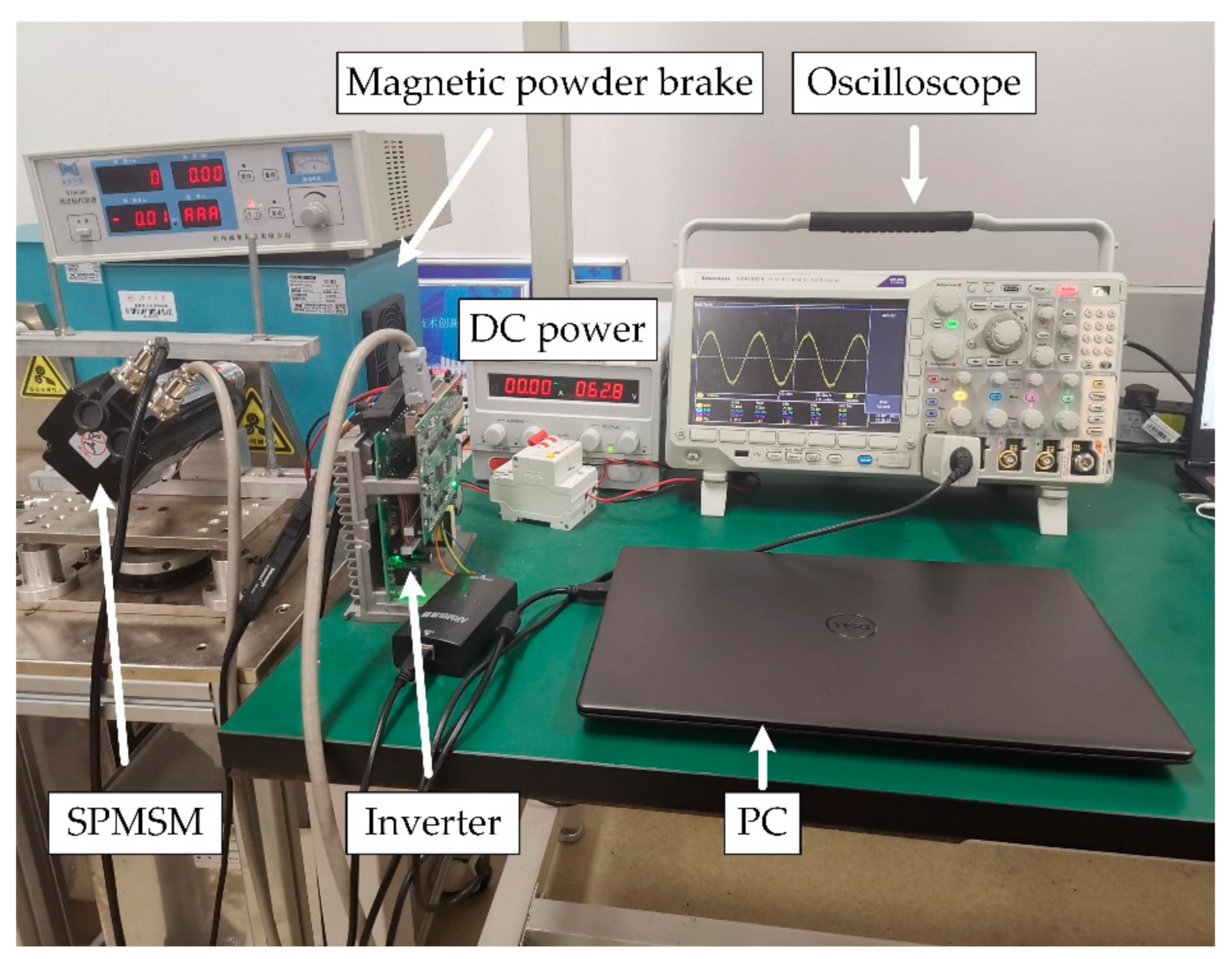
5. Experimental Results

The experimental platform is shown in Figure 9. The load is applied by a magnetic powder brake with high torque control accuracy. The power device of VSI is FSBB30CH60F. The switching frequency of the inverter is 12kHz. The experimental waveforms are observed by a Tektronix oscilloscope (Tektronix, (Oregon), Beaverton, U.S.). The main parameters of the prototype PMSM are shown in

Table 2. Design parameters of SPMSM.

Parameter	Value
DC-link voltage	60 V
Rated speed	600 rpm
Rated current	3 A
Number of pole pairs	4
Nominal d-axis inductance	2.8 mH
Nominal q-axis inductance	2.8 mH
Permanent magnet flux linkage	109.1 mWb
Stator winding resistance	1.86 Ω

and the electrical parameters of the inverter are shown in

Table 3. Characteristic parameters of voltage source inverter.

Parameter	Typical Value
Turn-on delay (Ton)	0.49 μs
Turn-off delay (Toff)	0.86 μs
Dead time (Tdead)	4 μs
Switching period (Ts)	83.3 μs
Voltage drop of the switching tube (Vsat)	2.75 V(max)
Voltage drop of the freewheeling diode (Vd)	2.4 V(max)

Note: Data from data sheet of FSBB30CH60F and T_I = 25 °C.

.

Comparative experimental tests of the proposed DP-CZD and the conventional DM-CZD under the field-oriented control and current predictive control for VSI nonlinearity compensation are given in this section.

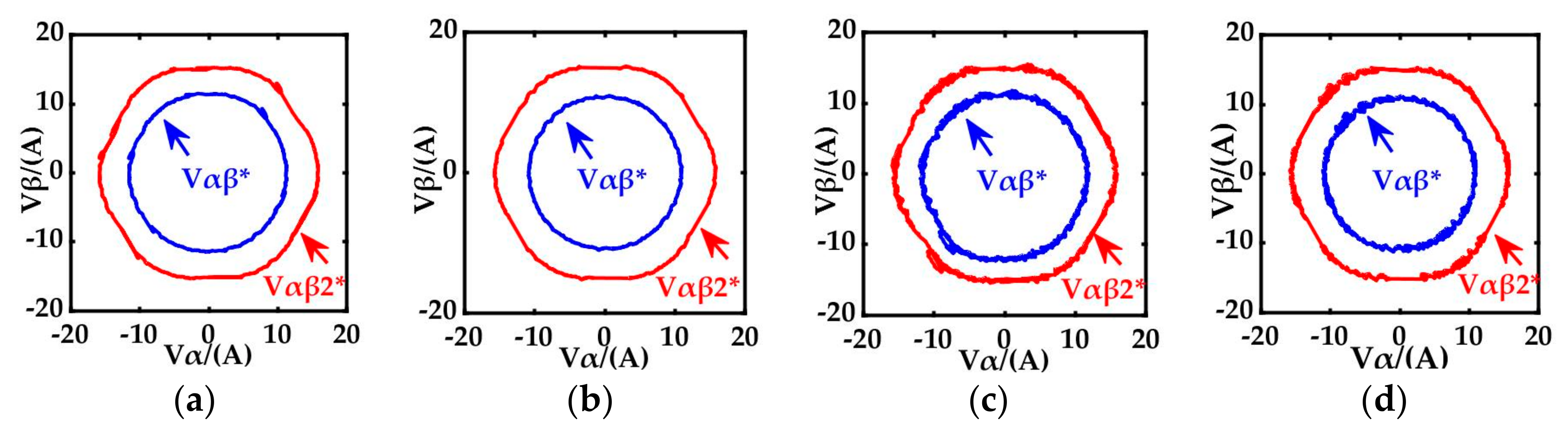
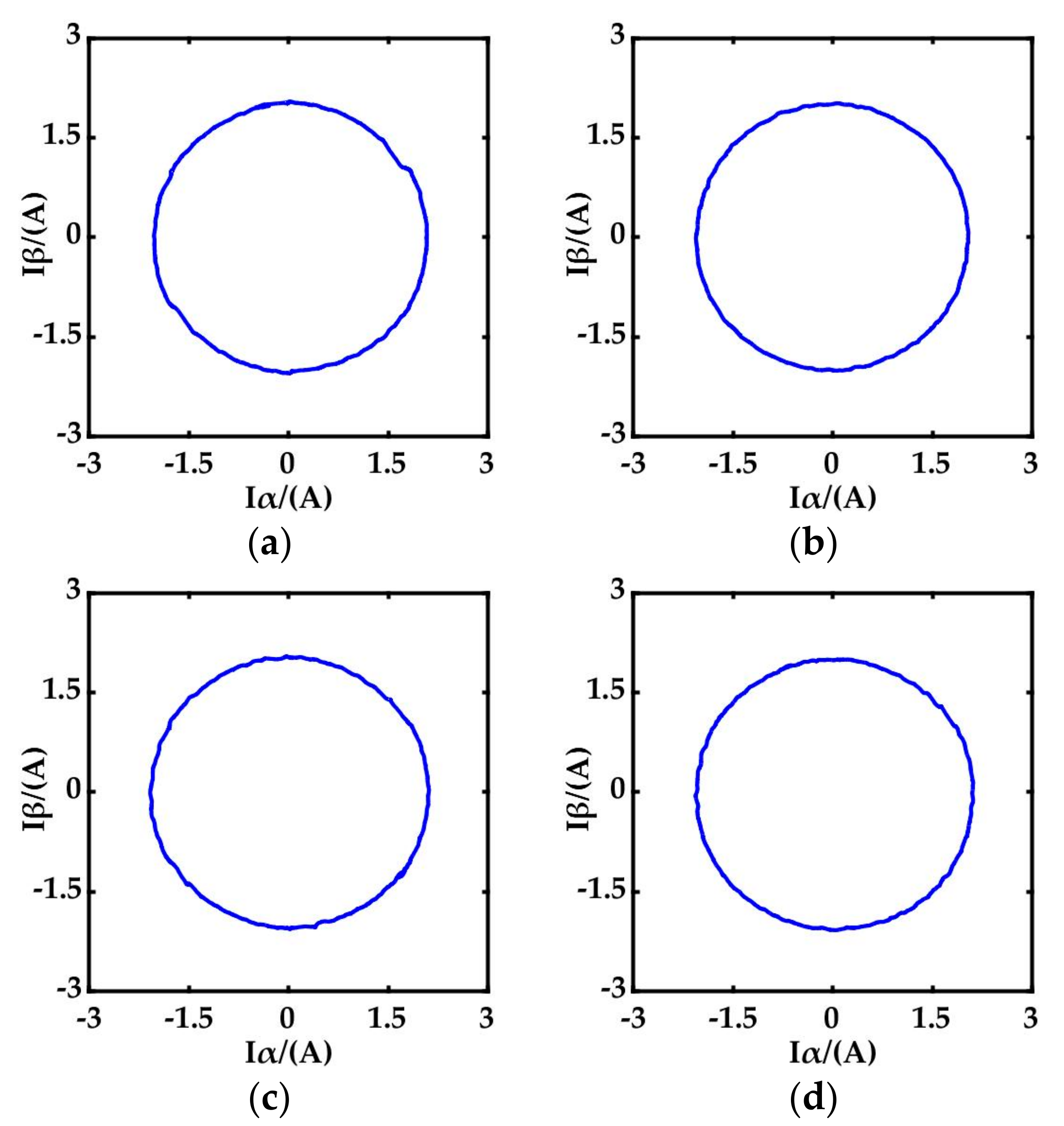
5.1. Evaluation of Steady State Performance

The results of VSI nonlinearity compensation under different frames are shown in Figure 10, Figure 11, Figure 12, Figure 13 and Figure 14. Figure 10 shows the αβ-axis reference voltages in different frames at 150 r/min. V_αβ* represents the αβ-axis voltages of $u_d^{*}$ and $u_q^{*}$, and V_αβ2* is the αβ-axis voltages of $u_{d2}^{*}$ and $u_{q2}^{*}$ in Figure 6 and Figure 7, respectively. Apparently, the V_αβ^* in Figure 10b,d is more orbicular than Figure 10a,c. Figure 10 shows that the voltage error is large and cannot be ignored. Consequently, the compensation of the VSI nonlinearity is necessary.

Figure 11 shows the phase A currents under different cases. From the fast Fourier transform (FFT) analysis results of the phase A currents shown in Figure 12, it can be seen that, with the VSI nonlinearity compensation through the proposed DP-CZD under the FOC system, the amplitude of the 5th harmonic and 7th harmonic reduce to 0.54% and 0.17% of the fundamental, respectively. For VSI nonlinearity compensation through DP-CZD under the current predictive control, the amplitude of the 5th and 7th harmonic reduce to 0.45% and 0.06% of the fundamental, respectively. Meanwhile, the total harmonic distortions in Figure 12b,d are smaller than Figure 12a,c.

Obviously, the circular of the αβ-axis currents in Figure 13b,d is also more orbicular than currents with VSI nonlinearity compensation using conventional DM-CZD in Figure 13a,c. Furthermore, the pulsation of currents in the dq-axis, $i_d\left(k\right)$ and $i_q\left(k\right)$, given in Figure 14b,d, have reduced from 0.28 A to 0.07 A, and 0.20 A to 0.08 A, respectively, compared with Figure 14a,c.

5.2. Evaluation of Dynamic Performance

Figure 15 shows the waveforms of dq-axis currents and rotor speed during ramp response and 1N∙m load. The slopes of ramp speed are −120 r/s and 360 r/s, respectively. It can be seen that the dq-axis currents in Figure 15a,c fluctuate sharply when the rotor speed changes. In Figure 15b,d, with the VSI nonlinearity compensation using proposed DP-CZD, the fluctuations of the dq-axis currents are reduced from 0.31 A to 0.08 A and 0.16 A to 0.06 A, respectively.

Figure 16 shows the waveforms of the dq–axis currents and rotor speed during step response and 1.5 N∙m load. The reference speed changes from 100 r/min to 350 r/min. It can be observed from Figure 16a,c that there is a large pulsation in dq-axis currents. In Figure 16b,d, the amplitudes of the dq-axis currents’ distortions have been reduced from 0.30 A to 0.09 A and 0.25 A to 0.12 A, respectively. Meanwhile, the fluctuation in rotor speed has been reduced from 4 r/min to 2 r/min, as compared in Figure 16a–c.

Figure 17 shows the waveforms of the dq–axis currents during load step response and 200 r/min. The q–axis current changes from 1.2 A to 2.9 A. It can be obviously seen form Figure 17a,c that the dq-axis currents have evident fluctuation. In Figure 17b,d, the pulsations of the dq–axis currents have been reduced from 0.30 A to 0.95 A and 0.21 A to 0.09 A, compared with Figure 17a,c. In general, according to the dynamic experimental results of Figure 15, Figure 16 and Figure 17, VSI nonlinearity compensation with proposed DP-CZD shows superior dynamic performance and improves compensation accuracy under a dynamic state.

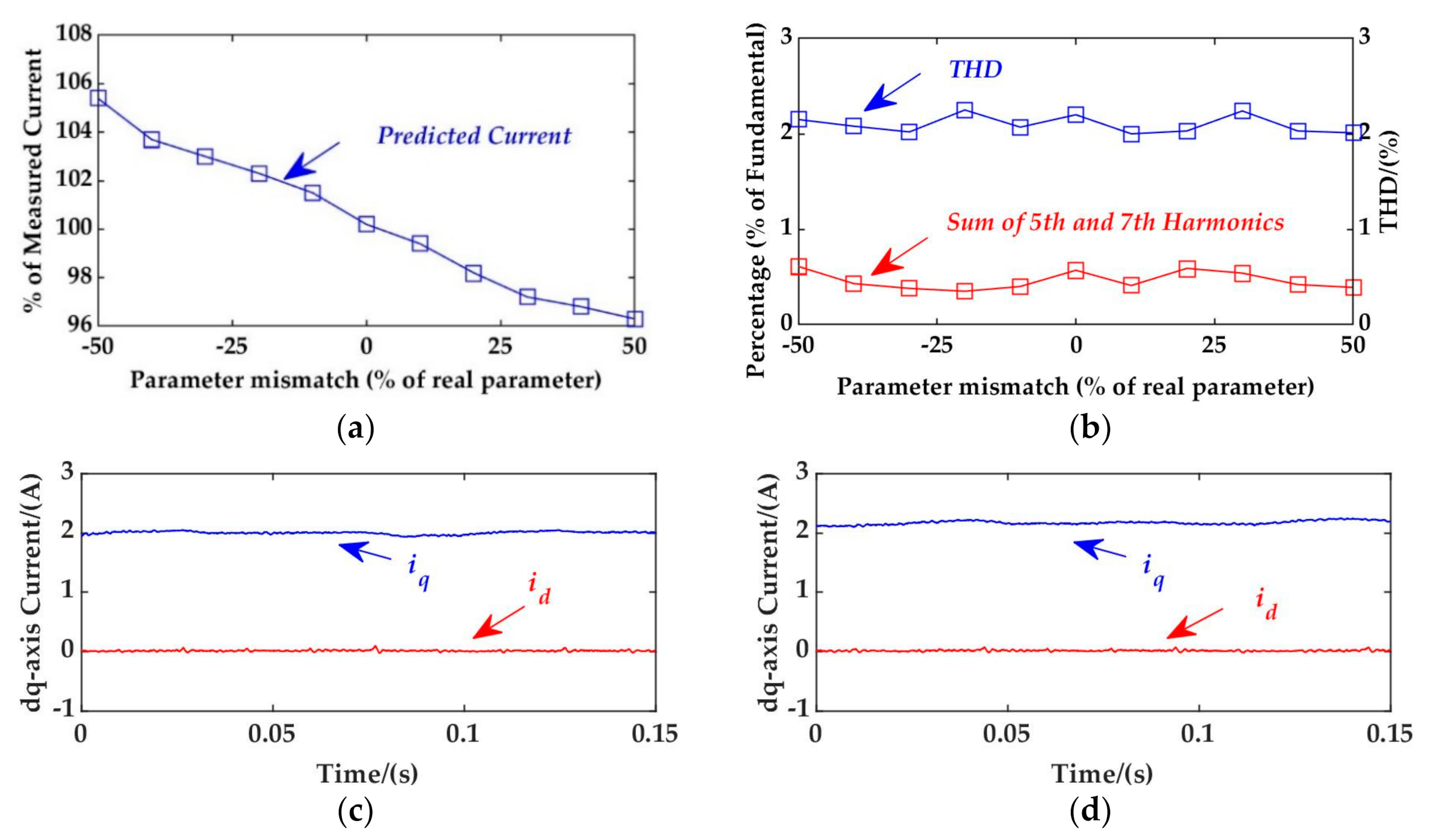
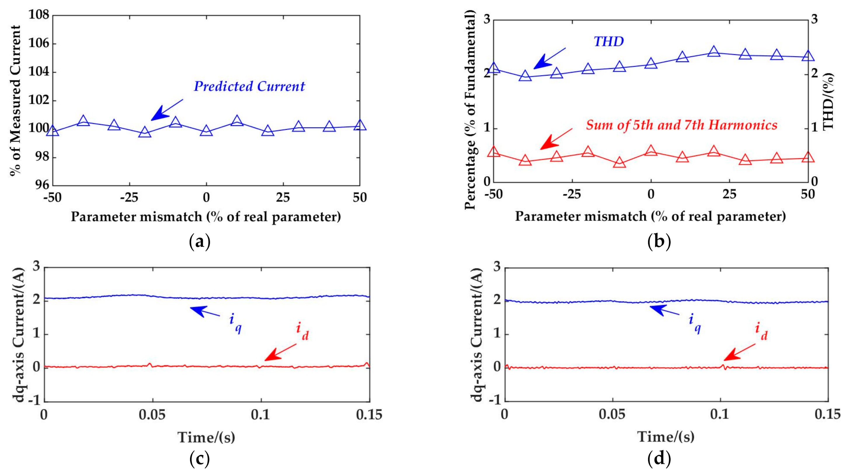
5.3. Evaluation of Robustness against Parameter Mismatches

Figure 18 shows the relationships between the current prediction errors and parameter mismatches. From Figure 18a, the RSE between predicted and real currents increases with P_R. With the increase in P_ψ, the values of the permanent magnet flux linkage ψ_f and the SE between the predicted and real currents increase in Figure 18b. Furthermore, the THD increases with P_L increase. The experiment results are consistent with simulation results in Figure 8. In order to prove that proposed DP–CZD has good robustness, experimental results for VSI nonlinearity compensation with proposed DP–CZD under parameters mismatch are shown in Figure 19, Figure 20 and Figure 21.

Figure 19, Figure 20 and Figure 21 show predicted and measured currents, THD, 5th and 7th harmonics in the case that the ratio of the percentage of mismatched parameters to real parameters varies from negative 50% to positive 50%.

From Figure 19, it can be seen that there is a steady state error between the measured and predicted phase currents due to mismatched stator winding resistance. The corresponding FFT results of the phase current under mismatched stator winding resistance are shown in Figure 19b, from which it can be found that the THD is around 2.1%, and the sum of the 5th and 7th harmonics is around 0.5% of the fundamental. The pulsations of dq–axis currents in Figure 19c,d are as small as in Figure 14b,d.

Figure 20a shows a steady state error between measured and predicted phase currents due to mismatched permanent magnet flux linkage, whose trend is consistent with Figure 8b. Furthermore, the THD is around 2%, while the sum of the 5th and 7th harmonics is around 0.5% of the fundamental in Figure 20b. It is clearly shown that the steady state error caused by mismatched stator winding resistance and permanent magnet flux linkage have no effect on VSI nonlinearity compensation using the proposed DP–CZD. The ripples of dq–axis currents in Figure 20c,d are as negligible as in Figure 14b,d.

Figure 21a shows that the steady state error between measured and predicted phase currents is near zero, which means mismatched stator inductance will not lead to a steady state error. In addition, the THD is around 2.1%, while the sum of the 5th and 7th harmonics is also around 0.5% of the fundamental in Figure 21b. The spikes of dq-axis currents in Figure 21c,d are as small as in Figure 14b,d. It can be seen from Figure 19, Figure 20 and Figure 21 that VSI nonlinearity compensation using the proposed DP–CZD shows a good robustness against parameter mismatches.

6. Conclusions

This paper proposes a VSI nonlinearity compensation method using DP-CZD for the suppression of disturbance voltage and current distortion in PMSM drive system, which can be employed in both field-oriented and current predictive controls. The proposed DP–CZD can effectively mitigate the influences of current clamping, current measurement noise, and control system delay in the polarity detection of the zero-crossing of phase current. Consequently, the accuracy of VSI nonlinearity compensation can be effectively improved. Besides this, the proposed DP–CZD does not need extra investment in hardware, and its effectiveness in compensating the VSI nonlinearity is verified on a prototype surface-mounted PMSM. It is found in experiments that under both the steady state and dynamic states, a much higher accuracy in the compensation of VSI nonlinearity is achieved with the proposed DP-CZD. In addition, it also shows a good robustness against parameter uncertainties, even if there is a 50% error in the electrical parameter values of PMSM. Since reference voltages can be well compensated by the proposed DP–CZD method, a further consideration is its application to torque ripple suppression, sensorless control and the parameter identification of PMSM drive systems, and relevant research will be reported in near future works.

The prototype SPMSM is fed and controlled by a servo drive board controlled by the MCU MKV31VF256VLL12, and all experimental verifications in this paper are carried out in this platform, which is shown in Figure 9. The design parameters of the tested SPMSM are shown in Table 2. In addition, the design parameters of the employed VSI are shown in Table 3. The DC-link voltage employed in the proposed method is obtained according to the measurement circuit in the servo board.

References

1. Li, L.; Xiao, J.; Zhao, Y.; Liu, K.; Peng, X.; Luan, H.; Li, K. Robust Position Anti-Interference Control for PMSM Servo System with Uncertain Disturbance. China Electrotech. Soc. Trans. Electr. Mach. Syst. 2020, 4, 151–160. [Google Scholar] [CrossRef]
2. Liu, K.; Zhu, Z.Q.; Zhang, Q.; Zhang, J. Influence of Nonideal Voltage Measurement on Parameter Estimation in Permanent-Magnet Synchronous Machines. IEEE Trans. Ind. Electron. 2011, 59, 2438–2447. [Google Scholar] [CrossRef]
3. Liu, K.; Zhu, Z.; Zhang, Q.; Zhang, J.; Shen, A. Influence of Inverter Nonlinearity on Parameter Estimation in Permanent Magnet Synchronous Machines. In Proceedings of the XIX International Conference on Electrical Machines—ICEM 2010, Rome, Italy, 6–8 September 2010. [Google Scholar] [CrossRef]
4. Feng, G.; Lai, C.; Mukherjee, K.; Kar, N.C. Current Injection-Based Online Parameter and VSI Nonlinearity Estimation for PMSM Drives Using Current and Voltage DC Components. IEEE Trans. Transp. Electrif. 2016, 2, 119–128. [Google Scholar] [CrossRef]
5. Shen, G.; Yao, W.; Chen, B.; Wang, K.; Lee, K.; Lu, Z. Automeasurement of the Inverter Output Voltage Delay Curve to Compensate for Inverter Nonlinearity in Sensorless Motor Drives. IEEE Trans. Power Electron. 2013, 29, 5542–5553. [Google Scholar] [CrossRef]
6. Martinez, D.I.; Rubio, J.D.J.; Vargas, T.M.; Garcia, V.; Ochoa, G.; Balcazar, R.; Cruz, D.R.; Aguilar, A.; Novoa, J.F.; Aguilar-Ibanez, C. Stabilization of Robots with a Regulator Containing the Sigmoid Mapping. IEEE Access 2020, 8, 89479–89488. [Google Scholar] [CrossRef]
7. Rubio, J.D.J.; Novoa, J.F.; Ochoa, G.; Mujica-Vargas, D.; Garcia, E.; Balcazar, R.; Elias, I.; Cruz, D.R.; Juarez, C.F.; Aguilar, A. Structure Regulator for the Perturbations Attenuation in a Quadrotor. IEEE Access 2019, 7, 138244–138252. [Google Scholar] [CrossRef]
8. Escobedo-Alva, J.O.; Garcia-Estrada, E.C.; Paramo-Carranza, L.A.; Meda-Campana, J.A.; Tapia-Herrera, R. Theoretical Application of a Hybrid Observer on Altitude Tracking of Quadrotor Losing GPS Signal. IEEE Access 2018, 6, 76900–76908. [Google Scholar] [CrossRef]
9. Rubio, J.D.J.; Martinez, D.I.; Garcia, V.; Gutierrez, G.J.; Vargas, T.M.; Ochoa, G.; Balcazar, R.; Pacheco, J.; Meda-Campana, J.A.; Mujica-Vargas, D. The Perturbations Estimation in Two Gas Plants. IEEE Access 2020, 8, 83081–83091. [Google Scholar] [CrossRef]
10. Aguilar-Ibanez, C.; Suarez-Castanon, M.S. A Trajectory Planning Based Controller to Regulate an Uncertain 3D Overhead Crane System. Int. J. Appl. Math. Comput. Sci. 2019, 29, 693–702. [Google Scholar] [CrossRef] [Green Version]
11. García-Sánchez, J.R.; Tavera-Mosqueda, S.; Silva-Ortigoza, R.; Hernández-Guzmán, V.M.; Gutiérrez, J.S.; Marcelino-Aranda, M.; Taud, H.; Marciano-Melchor, M. Robust Switched Tracking Control for Wheeled Mobile Robots Considering the Actuators and Drivers. Sensors 2018, 18, 4316. [Google Scholar] [CrossRef] [Green Version]
12. Urasaki, N.; Senjyu, T.; Kinjo, T.; Funabashi, T.; Sekine, H. Dead-Time Compensation Strategy for Permanent Magnet Synchronous Motor Drive Taking Zero-Current Clamp and Parasitic Capacitance Effects into Account. IEE Proc. Electr. Power Appl. 2005, 152, 845. [Google Scholar] [CrossRef]
13. Chen, L.; Peng, F.Z. Dead-Time Elimination for Voltage Source Inverters. IEEE Trans. Power Electron. 2008, 23, 574–580. [Google Scholar] [CrossRef]
14. Lin, Y.-K.; Lai, Y.-S. Dead-Time Elimination of PWM-Controlled Inverter/Converter without Separate Power Sources for Current Polarity Detection Circuit. IEEE Trans. Ind. Electron. 2009, 56, 2121–2127. [Google Scholar] [CrossRef]
15. Kim, H.-W.; Youn, M.-J.; Cho, K.-Y.; Kim, H.-S. Nonlinearity Estimation and Compensation of PWM VSI for PMSM under Resistance and Flux Linkage Uncertainty. IEEE Trans. Control. Syst. Technol. 2006, 14, 589–601. [Google Scholar] [CrossRef]
16. Liang, D.; Li, J.; Qu, R.; Kong, W. Adaptive Second-Order Sliding-Mode Observer for PMSM Sensorless Control Considering VSI Nonlinearity. IEEE Trans. Power Electron. 2018, 33, 8994–9004. [Google Scholar] [CrossRef]
17. Liu, K.; Zhu, Z.-Q. Online Estimation of the Rotor Flux Linkage and Voltage-Source Inverter Nonlinearity in Permanent Magnet Synchronous Machine Drives. IEEE Trans. Power Electron. 2014, 29, 418–427. [Google Scholar] [CrossRef] [Green Version]
18. Liu, T.; Li, Q.; Tong, Q.; Zhang, Q.; Liu, K. An Adaptive Strategy to Compensate Nonlinear Effects of Voltage Source Inverters Based on Artificial Neural Networks. IEEE Access 2020, 8, 129992–130002. [Google Scholar] [CrossRef]
19. Zhao, H.; Wu, Q.M.J.; Kawamura, A. An Accurate Approach of Nonlinearity Compensation for VSI Inverter Output Voltage. IEEE Trans. Power Electron. 2004, 19, 1029–1035. [Google Scholar] [CrossRef]
20. Bolognani, S.; Ceschia, M.; Mattavelli, P.; Paccagnella, A. Improved FPGA-Based Dead Time Compensation for SVM Inverters. In Proceedings of the Second International Conference on Power Electronics, Machines and Drives (PEMD), Edinburgh, UK, 31 March–2 April 2004. [Google Scholar] [CrossRef]
21. Kim, H.-S.; Kim, K.-H.; Youn, M.-J. On-Line Dead-Time Compensation Method Based on Time Delay Control. IEEE Trans. Control. Syst. Technol. 2003, 11, 279–285. [Google Scholar] [CrossRef]
22. Zhu, S.; Huang, W.; Yan, Y. A Simple Inverter Nonlinearity Compensation Method Using On-Line Voltage Error Observer. In Proceedings of the 2019 22nd International Conference on Electrical Machines and Systems (ICEMS), Harbin, China, 11–14 August 2019. [Google Scholar] [CrossRef]
23. Liu, G.; Wang, D.; Jin, Y.; Wang, M.; Zhang, P. Current-Detection-Independent Dead-Time Compensation Method Based on Terminal Voltage A/D Conversion for PWM VSI. IEEE Trans. Ind. Electron. 2017, 64, 7689–7699. [Google Scholar] [CrossRef]
24. Kim, S.-Y.; Lee, W.; Rho, M.-S.; Park, S.-Y. Effective Dead-Time Compensation Using a Simple Vectorial Disturbance Estimator in PMSM Drives. IEEE Trans. Ind. Electron. 2009, 57, 1609–1614. [Google Scholar] [CrossRef]
25. Attaianese, C.; Tomasso, G. Predictive Compensation of Dead-Time Effects in VSI Feeding Induction Motors. IEEE Trans. Ind. Appl. 2001, 37, 856–863. [Google Scholar] [CrossRef]
26. Abronzini, U.; Attaianese, C.; D’Arpino, M.; Di Monaco, M.; Tomasso, G. Steady-State Dead-Time Compensation in VSI. IEEE Trans. Ind. Electron. 2016, 63, 5858–5866. [Google Scholar] [CrossRef]
27. Li, Y.; Zhang, Z.; Li, K.; Zhang, P.; Gao, F. Predictive Current Control for Voltage Source Inverters Considering Dead-Time Effect. China Electrotech. Soc. Trans. Electr. Mach. Syst. 2020, 4, 35–42. [Google Scholar] [CrossRef]
28. Ben-Brahim, L. On the Compensation of Dead Time and Zero-Current Crossing for a PWM-Inverter-Controlled AC Servo Drive. IEEE Trans. Ind. Electron. 2004, 51, 1113–1117. [Google Scholar] [CrossRef]
29. Tang, Z.; Akin, B. Compensation of Dead-Time Effects Based on Revised Repetitive Controller for PMSM Drives. In Proceedings of the 2017 IEEE Applied Power Electronics Conference and Exposition (APEC), Tampa, FL, USA, 26–30 March 2017. [Google Scholar] [CrossRef]
30. Yao, Y.; Huang, Y.; Peng, F.; Dong, J.; Zhang, H. An Improved Deadbeat Predictive Current Control with Online Parameter Identification for Surface-Mounted PMSMs. IEEE Trans. Ind. Electron. 2019, 67, 10145–10155. [Google Scholar] [CrossRef] [Green Version]
31. Liu, K.; Zhang, J. Adaline Neural Network Based Online Parameter Estimation for Surface-Mounted Permanent Magnet Synchronous Machines. Proc. CSEE 2010, 30, 68–73. [Google Scholar] [CrossRef]
32. Wang, Z.; Yu, A.; Li, X.; Zhang, G.; Xia, C. A Novel Current Predictive Control Based on Fuzzy Algorithm for PMSM. IEEE J. Emerg. Sel. Top. Power Electron. 2019, 7, 990–1001. [Google Scholar] [CrossRef]
33. Zhang, X.; Hou, B.; Mei, Y. Deadbeat Predictive Current Control of Permanent-Magnet Synchronous Motors with Stator Current and Disturbance Observer. IEEE Trans. Power Electron. 2017, 32, 3818–3834. [Google Scholar] [CrossRef]
34. Li, Y.; Li, Y.; Wang, Q. Robust Predictive Current Control with Parallel Compensation Terms against Multi-Parameter Mismatches for PMSMs. IEEE Trans. Energy Convers. 2020, 1. [Google Scholar] [CrossRef]
35. Xu, C.; Zaikun, H.; Shuai, L. Deadbeat Predictive Current Control for Permanent Magnet Synchronous Machines with Closed-Form Error Compensation. IEEE Trans. Power Electron. 2020, 35, 5018–5030. [Google Scholar] [CrossRef]
36. Widrow, B.; Lehr, M. 30 Years of Adaptive Neural Networks: Perceptron, Madaline, and Backpropagation. Proc. IEEE 1990, 78, 1415–1442. [Google Scholar] [CrossRef]
Figure 1. Simulated waveforms of computed Dd and Dq, id and iq under id = 0 (γ = 0) control and 150 r/min. (a) Dd and Dq. (b) dq−axis currents.
Wevj 12 00017 g001
Figure 2. Voltage-source inverter (VSI) nonlinearity compensation with conventional DM-CZD. (a) Diagram of VSI nonlinearity compensation under FOC. (b) Diagram of extraction of d-axis high-frequency voltage.
Wevj 12 00017 g002
Figure 3. Waveforms of phase A current, Dd and Dq at 150 r/min. (a) Phase A current without compensation. (b) Phase A current and dq–axis currents after compensation with conventional DM–CZD. (c) Dd and Dq after compensation with conventional DM-CZD.
Wevj 12 00017 g003
Figure 4. Time delay in SVPWM implementation.
Wevj 12 00017 g004
Figure 5. Measured and predicted phase currents.
Wevj 12 00017 g005
Figure 6. VSI nonlinearity compensation for PMSM FOC system with proposed DP–CZD.
Wevj 12 00017 g006
Figure 7. VSI nonlinearity compensation for current predictive control of PMSM with proposed DP–CZD.
Wevj 12 00017 g007
Figure 8. Simulation results of relationship between current prediction errors and parameter mismatches. (a) Relative steady state error under mismatched stator winding resistance. (b) Steady state error under mismatched permanent magnet flux linkage. (c) THD under mismatched stator inductance.
Wevj 12 00017 g008
Figure 9. Test bench and electrical machines.
Wevj 12 00017 g009
Figure 10. αβ–axis reference voltages under i d = 0 , 150 r/min and 1N∙m load. (a) Compensation for PMSM FOC system with conventional DM–CZD. (b) Compensation for PMSM FOC system with proposed DP–CZD. (c) Compensation for current predictive control of PMSM with conventional DM–CZD. (d) Compensation for current predictive control of PMSM with proposed DP–CZD.
Wevj 12 00017 g010
Figure 11. Phase A currents under i d = 0 , 150 r/min and 1 N∙m load. (a) Compensation for PMSM FOC system with conventional DM–CZD. (b) Compensation for PMSM FOC system with proposed DP–CZD. (c) Compensation for current predictive control of PMSM with conventional DM–CZD. (d) Compensation for current predictive control of PMSM with proposed DP–CZD.
Wevj 12 00017 g011
Figure 12. Fast Fourier transform (FFT) results of phase A current at 150 r/min and 1 N∙m load. (a) Compensation for PMSM FOC system with conventional DM–CZD. (b) Compensation for PMSM FOC system with proposed DP–CZD. (c) Compensation for current predictive control of PMSM with conventional DM–CZD. (d) Compensation for current predictive control of PMSM with proposed DP–CZD.
Wevj 12 00017 g012
Figure 13. αβ–axis currents under i d = 0 , 150 r/min and 1 N∙m load. (a) Compensation for PMSM FOC system with conventional DM–CZD. (b) Compensation for PMSM FOC system with proposed DP–CZD. (c) Compensation for current predictive control of PMSM with conventional DM–CZD. (d) Compensation for current predictive control of PMSM with proposed DP–CZD.
Wevj 12 00017 g013
Figure 14. dq–axis currents under i d = 0 , 150 r/min and 1N∙m load. (a) Compensation for PMSM FOC system with conventional DM–CZD. (b) Compensation for PMSM FOC system with proposed DP–CZD. (c) Compensation for current predictive control of PMSM with conventional DM–CZD. (d) Compensation for current predictive control of PMSM with proposed DP–CZD.
Wevj 12 00017 g014
Figure 15. dq–axis currents and rotor speed during ramp response and 1 N∙m load. (a) Compensation for PMSM FOC system with conventional DM–CZD. (b) Compensation for PMSM FOC system with proposed DP–CZD. (c) Compensation for current predictive control of PMSM with conventional DM–CZD. (d) Compensation for current predictive control of PMSM with proposed DP–CZD.
Wevj 12 00017 g015
Figure 16. Currents and rotor speed during step response and 1.5 N∙m load. (a) Compensation for PMSM FOC system with conventional DM–CZD. (b) Compensation for PMSM FOC system with proposed DP–CZD. (c) Compensation for current predictive control of PMSM with conventional DM–CZD. (d) Compensation for current predictive control of PMSM with proposed DP–CZD.
Wevj 12 00017 g016
Figure 17. dq–axis currents during load step response and 200 r/min. (a) Compensation for PMSM FOC system with conventional DM–CZD. (b) Compensation for PMSM FOC system with proposed DP–CZD. (c) Compensation for current predictive control of PMSM with conventional DM–CZD. (d) Compensation for current predictive control of PMSM with proposed DP–CZD.
Wevj 12 00017 g017
Figure 18. Relationships between current prediction errors and parameters mismatches. (a) Relative steady state error under mismatched stator winding resistance. (b) Steady state error under mismatched permanent magnet flux linkage. (c) Total harmonic distortion (THD) under mismatched stator inductance.
Wevj 12 00017 g018
Figure 19. Test results under mismatched stator winding resistance. (a) Ratio of percentage of predicted current versus measured current. (b) THD, 5th and 7th harmonics of phase A current. (c) dq–axis currents under −50% stator winding resistance error. (d) dq–axis currents under 50% stator winding resistance error.
Wevj 12 00017 g019
Figure 20. Test results under mismatched permanent magnet flux linkage. (a) Ratio of percentage of predicted current versus measured current. (b) THD, 5th and 7th harmonics of phase A current. (c) dq–axis currents under −50% permanent magnet flux linkage error. (d) dq–axis currents under 50% permanent magnet flux linkage error.
Wevj 12 00017 g020
Figure 21. Test results under mismatched stator inductance. (a) Ratio of percentage of predicted current versus measured current. (b) THD, 5th and 7th harmonics of phase A current. (c) dq–axis currents under −50% stator inductance error. (d) dq–axis currents under 50% stator inductance error.
Wevj 12 00017 g021