Iron Loss Modelling of Electrical Traction Motors for Improved Prediction of Higher Harmonic Losses

Abstract

A Finite Element (FE) modelling approach is presented to account for the core losses in electrical machines that are generated by higher harmonic frequencies, for example those caused by Pulse Width Modulation (PWM) switching or by space harmonics due to the machine geometry. The model builds further on a post-processing calculation tool that was recently developed to take into account the magnetic skin effect in electrical steel laminations at high frequencies, and extends this by a more detailed loss analysis of the minor hysteresis loops that are caused by the higher harmonics. Further, these tools for high-frequency loss analysis are integrated into a complete electrical machine model with separate consideration of the major and minor loops. The modelling approach relies strongly on extensive magnetic measurement data of the electrical steel, in order to accurately predict the different loss components for minor hysteresis loops as a function of the DC bias field, frequency and amplitude of the minor loop. Results from the model are shown for an automotive traction motor, illustrating the losses caused by PWM harmonics and demonstrating the relevance of including the skin effect in these calculations.

1. Introduction

ArcelorMittal has developed iCARe^®, a specific product line of electrical steels which are optimised for automotive traction electrical machines. In order to further reduce the magnetic core losses of these electrical steels for wide frequency operation, research is ongoing on the modelling of various mechanisms of core loss dissipation. A robust prediction of these losses under realistic operating conditions of the machine remains challenging, as core losses are strongly influenced by a number of factors which are not yet completely understood. Losses measured on an electrical machine can be considerably higher than those expected from laboratory measurements on steel sheets, due to the presence of stresses, material degradation from production techniques, operation at high temperature, etc. Additionally, the presence of time- and space-harmonics, for example due to inverter-fed operation, will result in additional losses, possibly in combination with minor loops and the occurrence of skin effect in the laminations. It is the aim of this paper to present a loss modelling approach that takes into account skin effect and minor loops, whilst relying on methodologies that can be combined with commercial Finite Element (FE) software packages without the need to access FE formulations [1].

A well-established approach for the prediction of core losses is based on the separation of iron losses into a hysteresis, excess and eddy current loss component, in accordance to the statistical loss theory as described by Bertotti [2]. This methodology relies on loss descriptions for which the parameters are tuned, based on extensive magnetic measurement data on the electrical steel over a range of frequencies, and polarisation levels that reflect the wide operating range of traction motors. Typically, loss models that are based on the statistical loss theory are implemented in the frequency domain, i.e., the loss is calculated at each harmonic frequency separately and then summed over all frequencies to obtain the overall loss figure. The general methodology can be extended to also include the effect on losses from mechanical stresses, material degradation, etc., if appropriate experimental data is available [3]. However, when it comes to the prediction of losses caused by higher harmonics of the magnetic polarisation, the aforementioned model has its limitations as it does not take into account any skin effects within the laminations. Moreover, this model is generally based on an extrapolation of magnetic measurements at low frequencies and at zero bias fields.

As it is not realistic to develop extensive three-dimensional (3D) models of traction motors that include the detail of every lamination, in order to predict the skin effect, a number of simplified methodologies have been presented in literature. Many of these methodologies are based on conventional two-dimensional (2D) FE models assuming a non-conductive core, in combination with a one-dimensional (1D) model in the depth of the lamination to predict the flux distribution throughout the thickness of the lamination. In [4], such a 1D non-linear time stepping FE model was simulated at each element of the mesh as a post-processing calculation after the completion of the main time-stepping 2D analysis of a motor. This allowed for losses and skin effect to be calculated, requiring only a short additional calculation time. More elaborate schemes involve coupled 2D-1D FE calculations, where both models are analysed simultaneously [5] to allow for reaction fields from the eddy currents to be coupled back into the main 2D analysis at every node of the mesh. Such an approach, however, requires a double iterative scheme, leading to a significant increase in computation time and problems with convergence. The efficiency of this approach was improved in [6] by the direct integration of the 1D problem in the 2D FE formulations, avoiding the double iterative computation and leading to a significantly faster overall computation. A number of other homogenisation methodologies have been developed to couple a macroscopic FE model with a homogeneous core with a 1D representation of the lamination thickness. For example, in [7], the magnetic field and flux density distributions in the depth of the lamination are approximated by the use of periodic Fourier series, leading to additional terms in the main FE formulations, but not requiring an explicit meshed 1D model. Although many of the above coupled 2D-1D approaches lead to accurate predictions of the skin effect, they cannot be readily implemented by application engineers as they require adaptations to the FE code.

As an alternative to the FE schemes, for solving the non-linear 1D problem, a Finite Difference (FD) approach could be used [8,9], by dividing the lamination in a number of parallel layers that exhibit constant flux and current density. Such an analysis can easily be implemented as a postprocessing operation to the main 2D FE model using standardly available dynamic solvers. Alternatively, when it is acceptable to assume linear material properties and adopt a constant permeability, closed-form analytical equations can be used to predict the flux re-distribution and eddy current losses [10,11]. However, this potentially leads to an overestimate of the skin effect due to the absence of saturation. In [12], such an analytical model was used where an equivalent constant permeability was chosen according to the average flux density through the lamination, leading to eddy current loss predictions that agreed well with measurements. In [13], core losses are accounted for by introduction of equivalent magnetic field strengths that are responsible for generating the hysteresis, excess and eddy current loss. In this method, equations for the magnetic field related to the eddy-current loss are introduced to enforce an implicit dependency on the magnetisation curve of the material, and non-linearity and skin effects can thus be taken into account. The equations are tuned using fitting factors, which are estimated by comparing calculated dynamic hysteresis loops with experimental ones.

Rather than relying on 2D models, it is naturally also possible to assess the skin effect through the analysis of a 3D model of a single lamination. In [14], a comparison is made between a statistical loss model based on 2D calculations and a 3D model of a single lamination where eddy currents are explicitly taken into account. It was found that both models predict similar no-load losses of a high-speed Permanent-Magnet (PM) machine, because skin effect was relatively absent in this application. However, when iron losses under load and Pulse Width Modulation (PWM) control are evaluated, it was demonstrated that eddy-current losses calculated by the statistical method are considerable larger than those calculated by the 3D model. Similarly, hysteresis losses were underestimated by the statistical model, because a uniform flux density throughout the lamination is assumed. In [15], a comparison is made between a 2D-1D model and a 3D model of a single lamination, in order to investigate the effect of currents in the edges of the laminations that are ignored in the 2D-1D model. It was found that the accuracy of the 1D model can suffer at high frequencies and thick laminations. However, only lamination thicknesses in excess of 1.5 mm were examined, therefore, conclusions on automotive electrical steel grades could not be drawn from this work.

A considerable amount of research was also published in regard to the computation of the additional losses caused by minor hysteresis loops. In [16], it is assumed that a linear relationship exists between the hysteresis losses caused by the minor loops and the flux-density, and empirical correction factors are used to tune this model to experimental data. In [17], hysteresis, excess and eddy-current losses associated with each minor loop are calculated based on the loss coefficients that were obtained for the major loop, without additional tuning factor. The bias field at which minor loops occur and the skin effect that appears at high frequencies is accounted for in [10], where a linear analytical model is used to predict flux redistribution within the lamination. Hysteresis and eddy current losses are then calculated based on the calculated flux distribution within the lamination. Excess losses are obtained based on the excess losses at zero bias field and adapted for the changed permeability at the bias field. The effect of the DC-bias field is also taken into account in [18], where factors are introduced that give an increase in total iron loss, which are expressed as polynomial functions of the DC bias field. These functions must be tuned using measurement data at different amplitudes and frequencies of the harmonics, as well as at different levels of bias field, therefore also implicitly including the skin effect through fitting with high frequency measurements. Other approaches rely on hysteresis models that are able to predict the shape of the minor loops, in order to limit the number of measurements that are required. For example, a Preisach model is used in [19], a Jiles-Atherton model in [20], a graphical hysteresis model in [21,22] and an energetic model in [12,23].

In this paper, a core loss model that is implemented in the time-domain is discussed, which takes into account the appearance of skin effect and minor loops. Firstly, conventional statistical models based on frequency- and time-domain are described. Then, equations to calculate the losses caused by the skin effect are presented and compared with the output from magnetic measurements. Finally, simulations on a permanent magnet automotive traction motor are discussed.

2. Theoretical Analysis of Loss Models which do not Account for Skin Effect

The statistical loss theory, mentioned previously, is based on the concept of separating the core losses into hysteresis, excess and classical eddy current components [2]:

$${P=P}_{hyst}{+P}_{exc}{+P}_{class}$$

(1)

For fixed frequencies, the above equations can be re-written in terms of the energy-loss per cycle W = P/f

$${W=W}_{hyst}{+W}_{exc}{+W}_{class}$$

(2)

Hysteresis loss is often also referred to as quasi-static loss, because its energy-loss per cycle is not dependent on frequency. The classical and excess losses are often labelled as dynamic losses, as they are generated by electrical currents that are induced by time-varying magnetic fields in the material, and therefore strongly depend on frequency. The classical loss component can be derived by assuming that induced currents are homogeneously distributed throughout the thickness of the lamination, i.e., by ignoring the magnetic domain structure in the material. In order to account for the non-homogeneity of the induced currents, which is caused by the movement of the domain walls, the excess loss component was introduced.

Although the loss components are frequently calculated from the polarisation waveforms in the frequency domain, this study is focussed on equations in the time-domain. Equivalent formulations for the frequency domain can be found elsewhere [24]. Time-domain modelling requires the formulation of the instantaneous power loss, p(t), for periodic waveforms of the polarisation, which is then integrated over time to obtain the average losses.

2.1. Hysteresis Loss Component

Because the hysteresis loss component is not affected by the dynamics or shape of the polarisation waveform, it is only a function of the peak magnetic polarisation, J_p, and the fundamental frequency, f₀ [3]:

$$P_{hyst}{=W}_{hyst}\left(J_p\right)f_0{=s}_{hyst}{ J}_p^{\left({\alpha +\beta J}_p\right)}{f}_0$$

(3)

where s_hyst, α and β are fitting parameters that depend on the electrical steel grade and are determined via Epstein frame measurements. The hysteresis energy loss per cycle, W_hyst, can actually be directly measured under quasi-static conditions, as it is the only loss component that does not depend on the dynamics of the waveform. Hysteresis losses can only be calculated a posteriori, after the complete hysteresis loop has been closed, and thus a direct description as a function of time cannot be given. Further, it is possible to account for the effect of rotational magnetisation by adapting the above equation, which was derived for alternating magnetization [3]:

$$P_{hyst}\left(J_p,f\right)=s_{hyst}\left(1+\left({r(J}_p)-1\right)c\right)J_p^{\left({\alpha +\beta J}_p\right)}{f}_0$$

(4)

where c is the local flux–distortion factor (c = J_min/J_p) and r(J_p) is an empirical rotational loss factor, which must be determined via experiments.

2.2. Excess loss component

As described in the statistical loss theory, equations for excess losses are derived by considering the magnetisation process as the result of n simultaneously active magnetic objects that have a random distribution in the cross-section of the lamination. A formulation for instantaneous power dissipation from excess losses can be given by [19]:

$$p_{exc}\left(t\right)=\sqrt{{\sigma GSV}_0}{\left(\frac{{\mathrm{d}J}_p\left(t\right)}{\mathrm{d}t}\right)}^{1.5}$$

(5)

where σ is the electrical conductivity, G is a dimensionless constant (0.1356), S is the lamination cross-sectional area and V₀ is a parameter which depends on J_p.

2.3. Classical Loss Component

In the absence of skin effect, the instantaneous classical loss p_class(t), which is due to a homogeneous distribution of eddy currents flowing in the lamination, is given by [10,12]:

$$p_{class}\left(t\right)=\frac{{\sigma l}^2}{12}{\left(\frac{\mathrm{d}B}{\mathrm{d}t}\right)}^2\approx \frac{{\sigma l}^2}{12}{\left(\frac{\mathrm{d}J}{\mathrm{d}t}\right)}^2,$$

(6)

where l is the thickness of the lamination and B the flux density, which in practical terms can be considered to be identical to the polarisation, J.

2.4. Overall Core Loss Model

Combining the equations from the different core loss components, the total average core loss that results from an arbitrary periodic polarisation waveform with period, T_p, can be obtained as follows:

$${P=P}_{hyst}{+P}_{exc}{+P}_{eddy}{=s}_{hyst}\left(1+\left(r(J_p)-1\right)c\right)J_p^{\left({\alpha +\beta J}_p\right)}{f}_0+\frac{1}{T_p}{{\displaystyle \int }}_0^{T_p}{p}_{exc}\left(t\right)\mathrm{d}t+\frac{1}{T_p}{{\displaystyle \int }}_0^{T_p}{p}_{class}\left(t\right)\mathrm{d}t$$

(7)

3. Loss Modelling Taking Skin Effect into Account

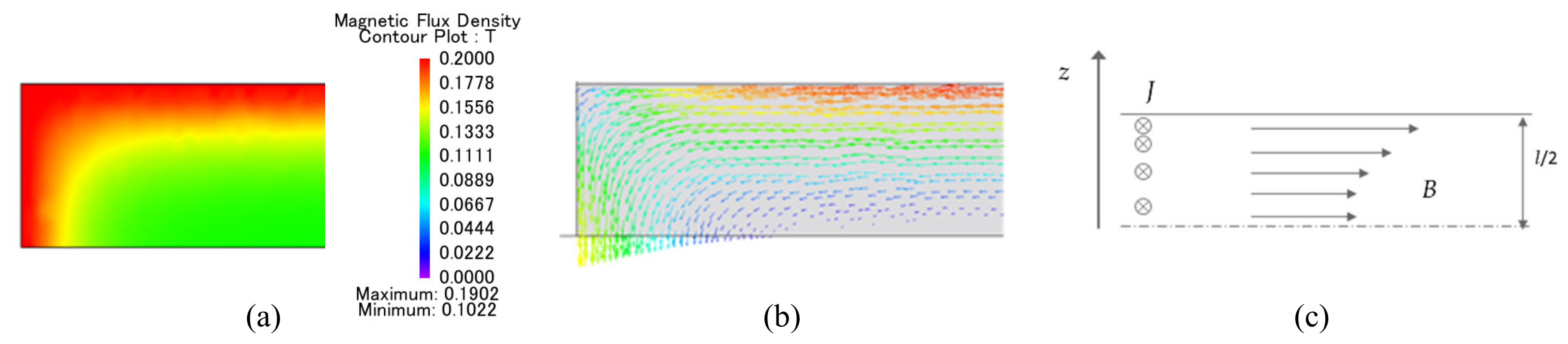
At elevated electrical frequencies, the skin effect will result in a redistribution of the flux within the lamination, therefore affecting all loss components previously described. This redistribution is shown in Figure 1a, which shows an FE calculation of the flux density in half of a 0.3 mm lamination, when a 10 kHz magnetic polarisation waveform with a peak value of 0.15 T is applied through the lamination. The corresponding current density distribution is shown in Figure 1b. When linear materials and sinusoidal waveforms are considered, the skin depth δ, i.e., the depth at which the polarisation is reduced to around 37% of the value at the surface of the lamination, can be calculated as [24,25]:

$$\delta =\frac{1}{\sqrt{\pi \mu f\sigma }}$$

(8)

where µ is the magnetic permeability. It could be shown that for a 0.3 mm thick 3%Si electrical steel which has a high peak value of permeability, the skin depth would already reach values smaller than half the thickness of the lamination at frequencies below 1 kHz, when a linear behaviour would be assumed. For small fluctuations of the polarisation around a DC bias, non-linearities can be ignored, and a constant permeability that is equal to the incremental permeability at the DC bias polarisation can be used. Therefore, the above equation can be used to estimate the skin depth in non-linear materials, provided the magnitude of the flux density remains small, as is often the case with higher harmonic disturbances.

In order to accurately calculate the distribution of magnetic flux and current within the lamination, it is necessary to compute Maxwell’s diffusion equation. For electrical steel laminations, the representation is often simplified to a one-dimensional problem in the direction of the lamination, with only half the lamination modelled, as schematically shown in Figure 1c. This leads to a simplified one-dimensional diffusion equation in the z-direction [8,9,13]:

$$\frac{{\partial }^{2}H(z,t)}{\partial z^2}=\sigma \frac{\partial B(z,t)}{\partial t}$$

(9)

for which a number of calculation methodologies exist. The use of the 1D modelling approach is valid, as long as the lamination exhibits large lateral dimensions compared to its thickness, because the return paths of the current, i.e., the end effects, are ignored.

3.1. Prediction of Eddy Current Loss Using Analytical Models

When the material exhibits a linear permeability and when a sinusoidal excitation is applied, it is possible to find an analytical solution for Equation (9) [10]:

$$H\left(z\right){=j\omega \sigma B}_p\frac{l}{2}\frac{\cosh \left(kz\right)}{k \sinh (kd/2)}, \mathrm{with} k=\frac{1+j}{\sqrt{2}}\sqrt{\omega \sigma \mu }$$

(10)

where ω is the electrical pulsation, and B_p is the peak value of the average flux density through the material. The resulting eddy current loss density can then be calculated as follows [10]:

$$W_{class}\left(J_p,f\right)=\frac{\mathsf{\pi }}{2}\frac{{\lambda J}_p^2}{\mu }\frac{\sinh \lambda -\sin \lambda }{\cosh \lambda -\cos \lambda }, \mathrm{with} \lambda =\sqrt{{\pi \sigma \mu l}^{2}f}.$$

(11)

3.2. Non-Linear Post-Processing Calculation Using a Finite Difference Modelling

A non-linear calculation methodology of the 1D problem has been derived in [8,9], by dividing the lamination in a number of layers with constant flux and current densities, as given in Equation (12):

$$\begin{gathered} \frac{{\mathrm{d}B}_1}{\mathrm{d}t}=\frac{{8H}_2{-7H}_1{-H}_3}{{2\sigma h}^2}+\frac{3\left(N-1\right)}{w_{1}S}u\left(t\right) \\ \frac{{\mathrm{d}B}_i}{\mathrm{d}t}=\frac{H_{i-1}{-2H}_i{+H}_{i+1}}{{\sigma h}^2}, (i=2,\dots ,N-1) \\ \frac{{\mathrm{d}B}_N}{\mathrm{d}t}=\frac{{2(H}_{N-1}{-H}_N)}{{\sigma h}^2} \end{gathered}$$

(12)

where

• B₁, B₂, ..., B_N are the flux densities in each of the N layers,
• H₁, H₂, …, H_N are the magnetic fields in each layer,
• h is the thickness of each layer,
• u(t) is the applied voltage over the winding with w₁ turns,
• and S is the cross-sectional area of the core.

Within each layer, the normal non-linear constitutive relationships are valid. As this methodology requires the solution of transient differential equations, dynamic solvers are required which are available in, for example, Python or Matlab/Simulink.

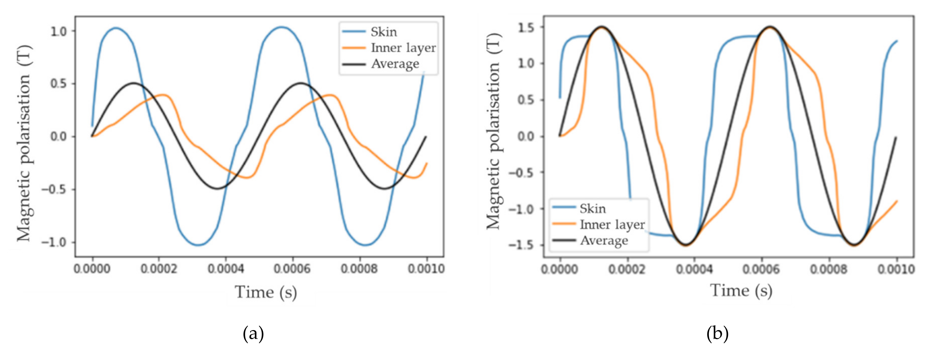
As an example of the result from this methodology, Figure 2a shows the magnetic polarisation waveforms in the inner and outer layers of an electrical steel with 0.3 mm thickness, when an average sinusoidal flux-density of 0.5 T at 2 kHz is applied. Here, a clear skin effect can be noticed, with a larger polarisation near the outer edge, a phase shift between polarisation waveforms throughout the thickness and strong non-linear behaviour, even though the total flux through the lamination is forced to be sinusoidal. Figure 2b shows similar waveforms when the average polarisation is 1.5 T at 2 kHz. In this case, however, the material starts to saturate near the edge of the lamination, such that the peak polarisations near the skin cannot rise above the average value, resulting in an identical peak value throughout the lamination. However, non-linearity and phase differences between the waveforms are apparent.

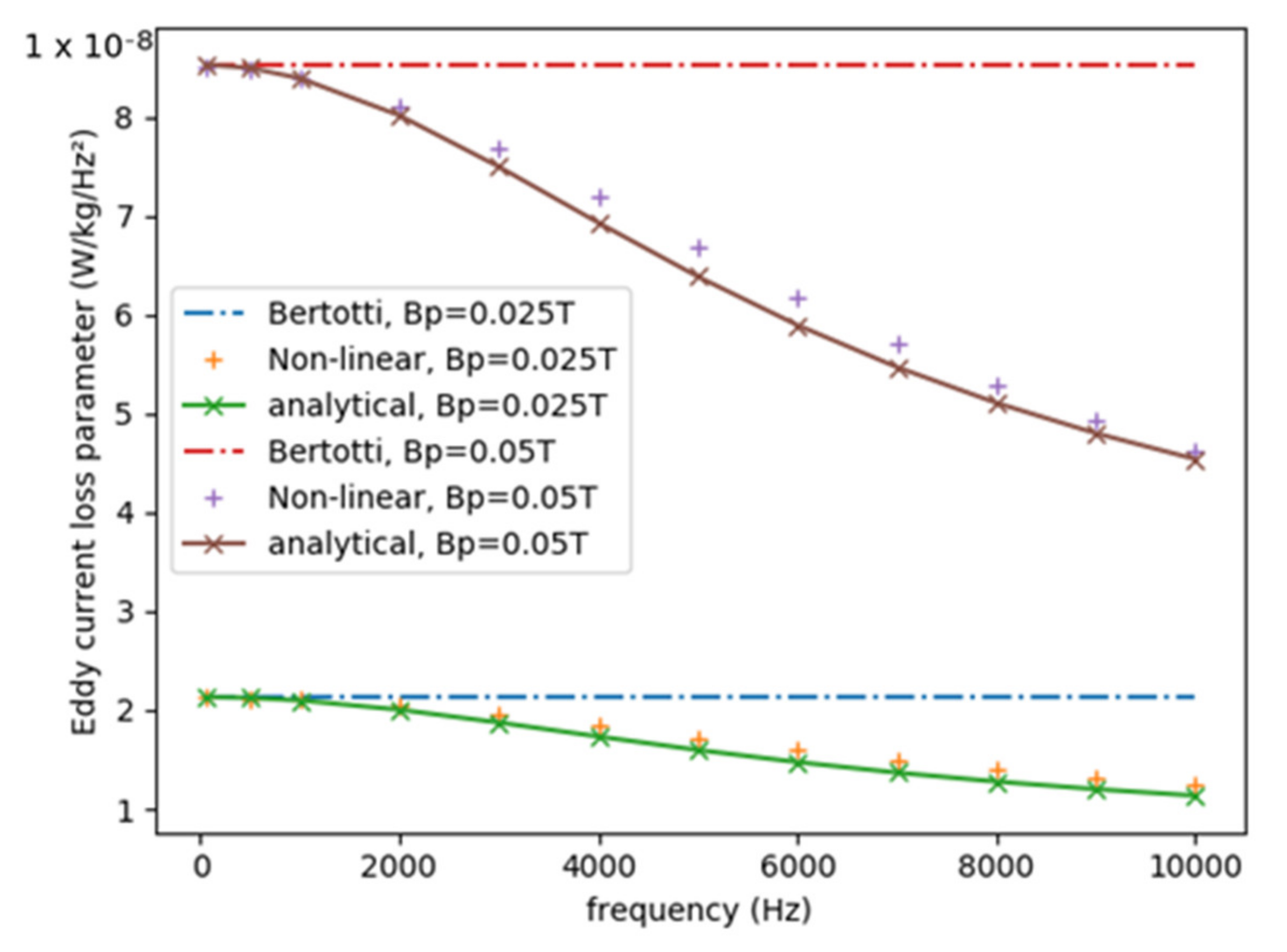
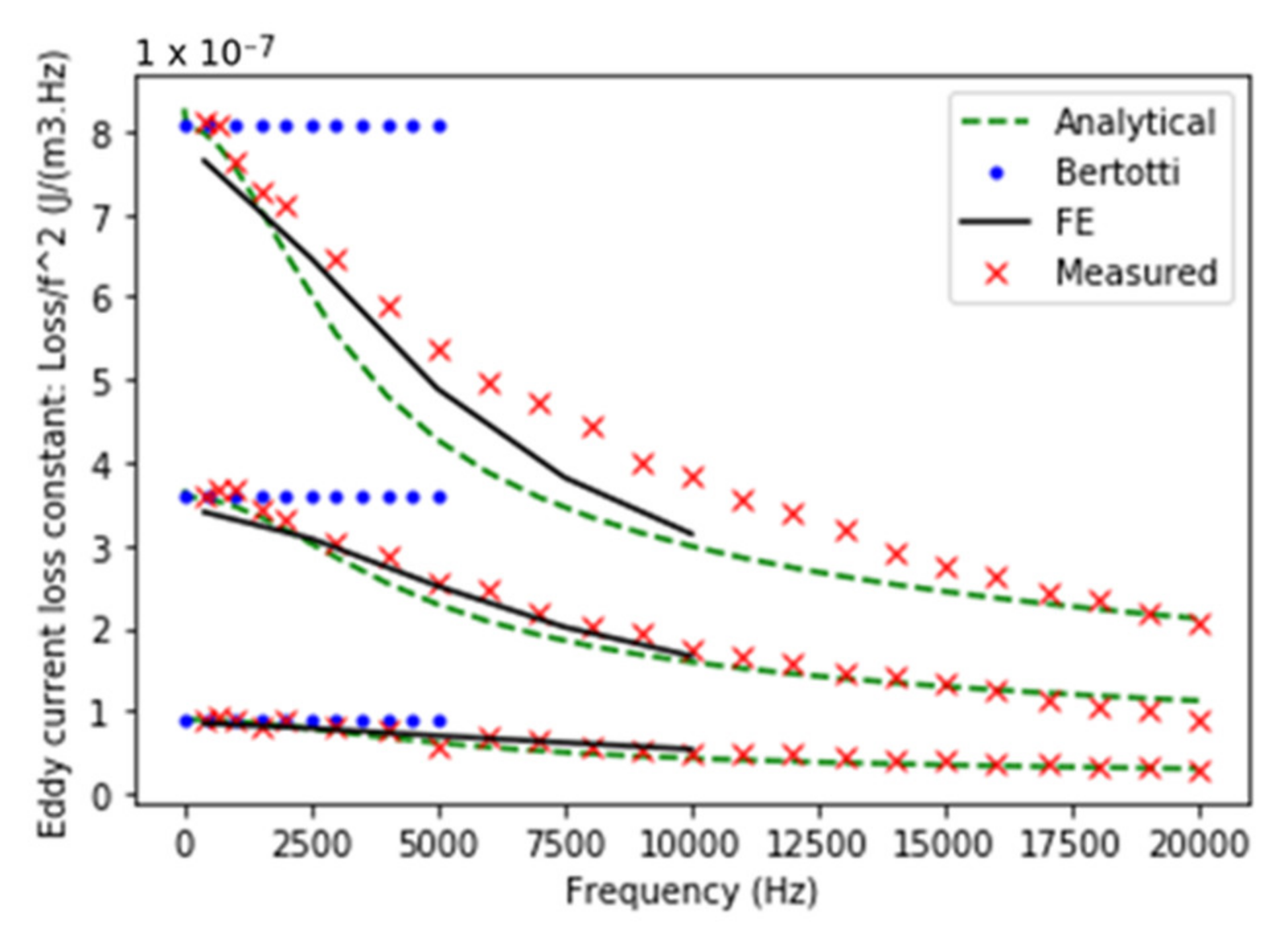
Having calculated the flux-density distribution, it becomes possible to predict the current density distribution and the resulting eddy-current losses. Figure 3 compares the loss constant for the previously defined calculation methodologies, i.e., the classical Bertotti calculation, the linear analytical formulation and the non-linear formulations, for two different averaged flux-density waveforms that are applied to the material. It can be seen that for low frequencies, in the absence of skin effect, the three methods give identical results. At high frequencies, however, the analytical and non-linear calculations both predict lower losses compared to the situation, when no skin-effect would be present. In other words, due to the skin effect, the current density in the material will not increase linearly any more with frequency, resulting in a slower increase in losses with frequency than would be expected without skin effect.

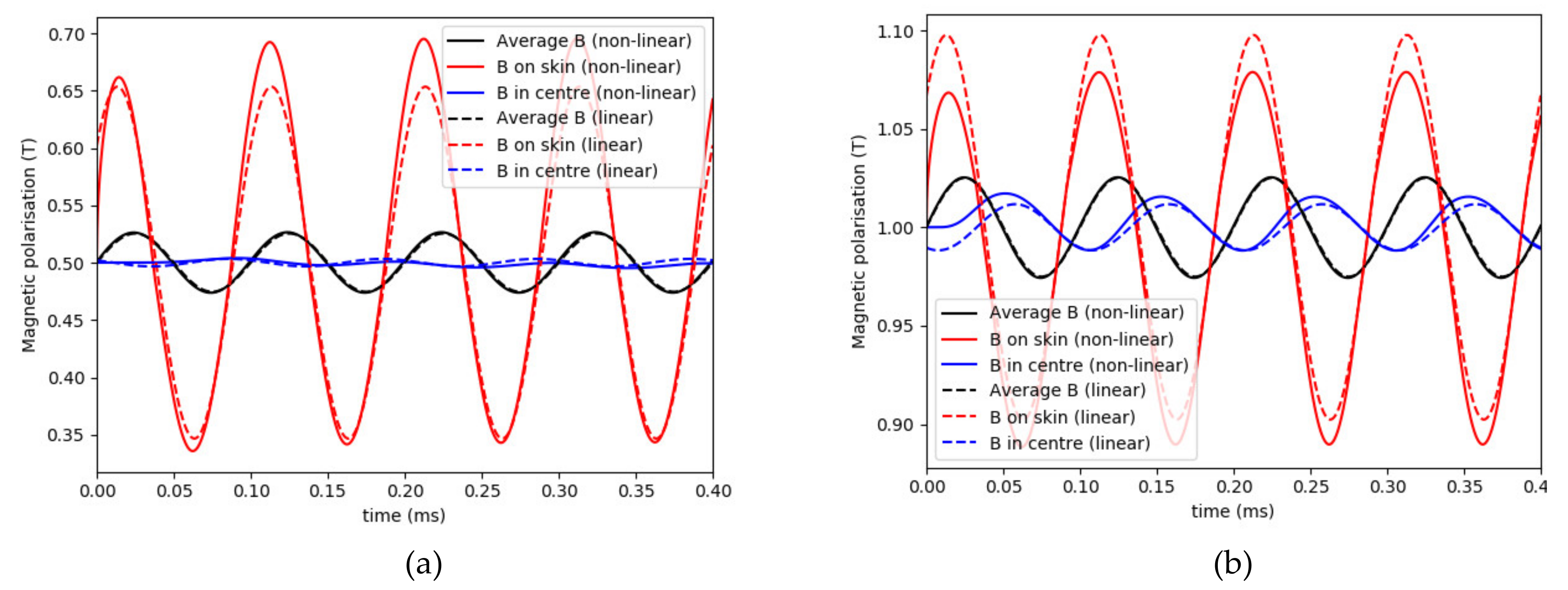
As the previous figure showed a good agreement between the linear and non-linear analysis for waveforms with small amplitude, Figure 4a,b compares magnetic polarisation waveforms in the skin and near the centre of the material, for high-frequency polarisation waveforms with small amplitudes. Further, a DC bias polarisation was added to the waveforms in the figure, in order to make the waveforms more representative for higher harmonics, for example, due to switching frequencies. As can be seen, for these small amplitudes, both linear and non-linear models predict similar polarisation waveforms, suggesting that a non-linear analysis may not be required and that the analytical calculation methodology could be sufficient. It can also be noted from the figures that a transient effect is present in the solution of Equation (12), such that a few periods must be simulated to obtain a stable steady-state solution.

3.3. FE Modelling of Eddy Current Loss

Finally, commercial FE packages can also be used to account for the skin effect. Certain software have implemented the approach where conventional 2D models with homogeneous material properties are operated in combination with a 1D model at each node of the model. This coupled 2D-1D modelling approach thus allows the calculation of eddy current losses for arbitrary transient excitation, taking into account non-linearities and also allowing coupling between eddy current losses with the field calculation itself. However, the models are generally available as a black-box tool predicting eddy-current loss only, and it is not possible to assess the actual flux density distribution in the depth of the lamination. Further, the computation may suffer from long computation times and convergence problems. Naturally, apart from the 2D-1D analysis mentioned above, accurate predictions can also be obtained through complete 3D modelling of the lamination, although this would involve a large computational cost.

3.4. Increase in Hysteresis and Excess Loss Due to Skin Effect

As a result of the skin effect, the magnetic polarisation is redistributed across the thickness of the lamination. Because the hysteresis loss is dependent on the peak polarisation at each point in the material, the hysteresis loss density is no longer homogeneous within the lamination. In this case, the hysteresis energy loss per cycle is to be calculated by averaging the loss across the thickness [10]:

$$W_{hyst}(J_p, f)=\frac{1}{l}{{\displaystyle \int }}_{-l/2}^{l/2}{s}_{hyst }{J}_p{\left(z\right)}^{{(\alpha +\beta J}_p\left(z\right))}\mathrm{d}z$$

(13)

with α, β and s_hyst given in Equation 3 and derived from low-frequency measurement results, where skin effect can be ignored. As hysteresis loss density generally increases with increasing polarisation (i.e., normally α+βJ_p > 1), skin effect is expected to result in an increased hysteresis loss. This may lead to only a small increase in total losses, however, as dynamic losses are normally dominant at high frequencies.

In fact, it is expected that the major hysteresis loop will not cause considerable skin effects and that losses can still be calculated in the conventional way, unless the fundamental frequency is sufficiently high. Minor loops, however, would always require some assessment of the skin effect. Further, as will be shown later, the parameters that describe hysteresis are sufficiently different for minor and major loops, such that a separate treatment of major and minor loops is necessary.

In this study, excess losses are assumed to be independent of the skin effect and only affected by the peak polarisation of the loop [10]. Further, for the assessment of minor loops, it is assumed that the coefficient, V₀, that is used to calculate the excess loss (Equation (5)) depends on the incremental permeability at the point where the minor loop and major loops are connected. For small amplitudes of the minor loop, the following equation can then be used [10]:

$$V_0{(J}_m{,J}_b)\approx V_0{(J}_m{,J}_b=0)\frac{\left|{\mu (J}_m{,J}_b=0)\right|}{\left|{\mu (J}_m{,J}_b)\right|}$$

(14)

where J_m and J_b are the peak amplitude and DC bias polarisation of the minor loop, respectively.

4. Global Modelling Approach

The global approach for the calculation of all core losses in an electrical machine is schematically shown in Figure 5. The approach is based on a FE model of the machine, which is simulated for a single electrical period using a large number of timesteps. Then, using a post-processing script, the waveforms of magnetic field and polarisation are constructed in each mesh element by collecting the solutions at different timesteps. This allows for the different loss components to be calculated in each element of the mesh, based on the time-domain formulations given previously in Section 2. Key to this methodology is access to measurement data on the modelled electrical steel, in order to derive material-specific core loss parameters, and also to establish the magnetisation curve that is to be used in the FE model. As previously reported for frequency-domain core loss models [3], the modelling approach can be further extended to account for the effects of mechanical stresses and material degradation, for example, due to cutting the motor laminations or operation at high temperatures.

For this study, the polarisation waveforms that are obtained for each element were subdivided into the major and minor loops, which were treated differently. Where the major loop is analysed according to the standard approach, the calculations for the minor loops include skin effect and are based on specific parameters for the calculation of quasi-static hysteresis loss.

5. Experimental Verification

In order to verify the loss formulations discussed in Section 3, and to validate the overall modelling approach as explained in Section 4, laboratory measurements were performed on a 0.3 mm thick 3%Si electrical steel for automotive applications. Additionally, quasi-static magnetic measurements were conducted for small-amplitude waveforms superimposed on a DC bias polarisation, in order to derive hysteresis fitting parameters for the minor loop analysis. Finally, a 50 Hz waveform with superposed harmonics was measured and compared with simulation results.

5.1. Sinusoidal Waveforms Without DC Bias

Conventional magnetic measurements were carried out for sinusoidal polarisation waveforms with an amplitude up to 0.15 T, and a frequency up to 20 kHz. From the total measured losses, the component that is due to eddy currents was derived as follows:

$$P_{eddy}{=P}_{measured}{-P}_{hyst\_skin}{-P}_{exc}$$

(15)

where P_{hyst_skin} refers to the hysteresis losses that have been corrected for the skin effect, and P_exc refers to the excess loss based on the average flux density in the lamination. Figure 6 shows a comparison between the eddy current loss constant, k_eddy, that was obtained from measurement and various calculation methodologies, where k_eddy was defined as the volumetric loss divided by the square of the frequency. It is clear that the downward slope of the eddy current losses with frequency is predicted by both the FE and analytical methods. The classical analysis is given by Equation (6) as it appears in the method from Bertotti, however, this overestimates the eddy current losses at high frequencies because the skin-effect is ignored.

5.2. Quasi-Static Measurements at DC Bias

In order to investigate the hysteresis loss that is dissipated in minor loops, measurements were conducted where quasi-static minor loops were generated for a range of amplitudes and DC bias levels. Because the measurement system is unable to measure a DC bias field, a slow-varying waveform was used, with the minor loop occurring at the peaks of this loop, as shown in Figure 7a. Figure 7b shows the resulting minor loops for an amplitude of 0.05 T with different bias values. As can be seen from the area of the respective loops, the hysteresis loss of the minor loop increases significantly with an increase in the DC bias field. Therefore, a mapping was obtained through measurements of a range of amplitudes and DC bias fields, to predict hysteresis loss of minor loops as a function of amplitude and bias field for future analysis.

5.3. Verification on a Waveform with High-Frequency Harmonics

In order to assess the overall modelling approach, an Epstein frame was used to measure core losses when the material was subjected to a 50 Hz, 0.9 T waveform, generated via a PWM scheme with a switching frequency of 4 kHz. The measured BH-loop is shown in Figure 8a, whereas the measured polarisation waveform is shown in Figure 8b. On this figure, the fluctuations that result in minor loops, and for which separate calculations are run, are indicated in red. The results of this analysis are summarised in

Table 1. Comparison of loss predictions for the data shown in Figure 8, for which a total loss of 0.967 W/kg was measured.

Methodology	Total Loss
Frequency-domain	1 W/kg from which 0.97 W/kg at the first harmonic
Time-domain without skin effect	0.97 W/kg
Time-domain with skin effect and minor loops	0.95 W/kg from which 0.15 W/kg at all minor loops

for different calculation methods. Here, it can be seen that for this example, all calculations provide a satisfactory answer. However, since the frequency-domain model predicts almost all of its power loss to be at the fundamental frequency, it does not properly separate losses. The model which includes a separate calculation for minor loops is the only one that can correctly separate losses, as it was measured that the presence of the harmonics added around 15% of losses.

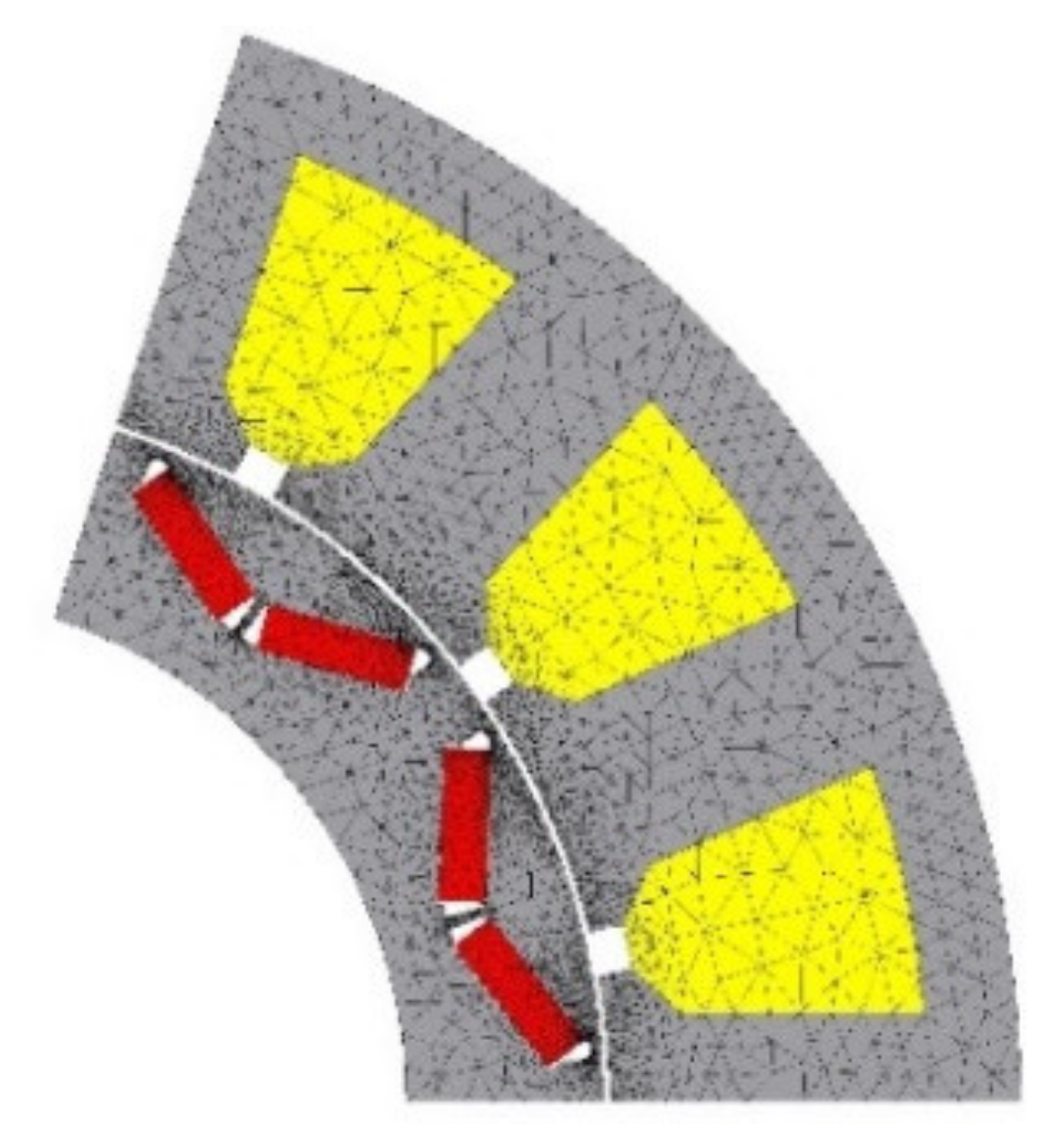
6. Application to Loss Modelling of Automotive Traction Motor

Figure 9 shows the model of an electrical machine that will be used as a reference for the analysis of the loss modelling approach. This 10-pole interior permanent magnet (IPM) machine was designed for an automotive traction application, and its specifications are given in

Table 2. Motor specifications.

Specification	Value
Outer diameter	195 mm
Axial length	171 mm
Nominal power	50 kW
Maximum torque	150 Nm
Maximum speed	12000 rpm

. In order to maximise the torque, a fractional slot topology with concentrated windings was used, resulting in considerable space-harmonics. The magnetic core is made from an electrical steel from the ArcelorMittals iCARe^® range that was selected for its low losses at elevated frequencies. As shown in Figure 9, the symmetry of the geometry is used to model only one pole-pair of the machine. For this machine, a previous study showed that the calculation of the skin effect did not significantly change the total core loss behaviour when the motor is supplied by sinusoidal waveforms. For this analysis, the motor was simulated at 4800 rpm, and supplied with a three-phase PWM waveform with a carrier frequency of 16 kHz, by using the standard library function that is implemented in the JMAG software. A timestep of 4.1 µs was used for the simulation.

For the analysis of core losses, a comparison was made between three models. Firstly, a conventional post-processing approach based on the statistical loss model in the frequency domain was used, as described in [3]. A second post-processing model was based in the time-domain, as described by Equation (7). For these first two models, skin effect was not taken into account and minor hysteresis loops were not separately analysed, although they do appear as higher harmonics of the flux density and are therefore included in the calculation of eddy current and excess losses. The third model consists of a time-domain model, with skin effect and minor loops explicitly accounted for. The skin effect was implemented using the tools available in the JMAG software, such that the reaction field is included in the main FE analysis. However, eddy current losses were calculated in post-processing, in order to allow a separate analysis of the major and minor loops according to the discussion in Section 3. The total core losses that are calculated by these three models are compared in

Table 3. Motor core loses calculated using different methodologies.

Methodology	Total Core Loss
Frequency-domain	546 W
Time-domain without skin effect	665 W
Time domain with skin effect and separate minor loop calculation	678 W

.

From the results, the difference between the frequency-domain and time-domain models can be noted, with a higher loss estimation for the time-domain models, although both models ignore skin effect and minor loops and are based on the same post-processing data. It is expected that this difference stems from the fact that loss calculation in the frequency-domain model is calculated from the superposition of all harmonics, which are treated independently, without taking their phase differences into account [18]. For this example, it appears that the hysteresis loss only increased by 1.5% when the hysteresis of the minor loops was taken into account. Further, the modelling allows for the calculation of the additional losses generated by the higher harmonics due to the PWM scheme, which appears to be around 15% of total core losses.

7. Conclusions

A framework has been described to predict iron losses of electrical machines, including skin effect and the presence of minor loops. The modelling approach was applied to an electrical steel from ArcelorMittal’s iCARe^® range, which is a portfolio of electrical steels specifically developed to satisfy the demanding requirements of automotive traction applications. Laboratory magnetic measurements at high frequencies showed good agreement with the theoretical behaviour of the material at high frequencies. Further, FE calculations were carried out to predict losses in an automotive traction motor. This showed that a time-domain model may lead to somewhat different results compared to a frequency-domain model, which is based on linear superposition of the contribution of the individual harmonics. It could further be concluded that the explicit calculation of skin-effect and minor hysteresis loops did not affect the loss prediction considerably for this specific machine geometry and control. For the analysed case, it could be shown that the harmonics that are generated by the of PWM control add an additional 15% of core losses.