
A DNN Architecture Generation Method for DDoS Detection via Genetic Alogrithm

Abstract
:1. Introduction
- With the access of various devices to the network and the emergence of more network services [10,11,12], DDoS attacks are becoming more secretive and changeable and can cause more significant losses [13,14,15,16,17]. For some networks, it is necessary to select a particular model to prevent DDoS attacks [18,19] and constantly adjust the model to identify new DDoS attack types or even reconstruct the model to detect rapidly changing DDoS attack patterns [20]. In these scenarios, the model’s construction needs experienced researchers. Frequent model construcution will consume many resources [21].
- This paper uses the GA to generate a model architecture while minimizing human intervention. In some scenarios, the proposed method can find a model with good performance in a limited time to deal with the problem of DDoS detection.
- This paper uses the model generated, some existing advanced DNN models and some advanced machine learning models to experiment on the same dataset. This paper evaluates theses models in terms of precision, recall, F1-score and accuracy. The analysis results show that the models generated by the proposed method have better performance than the existing methods studied in this paper.
- In addition to the CICDDoS2019 dataset, this article also conducted experiments on two other datasets, and the models generated by the proposed method still perform well.
- Six datasets are used to evaluate the best model generated by the method proposed in this paper and the best model generated by existing methods. The results show that the model generated in this paper has stronger generalization.
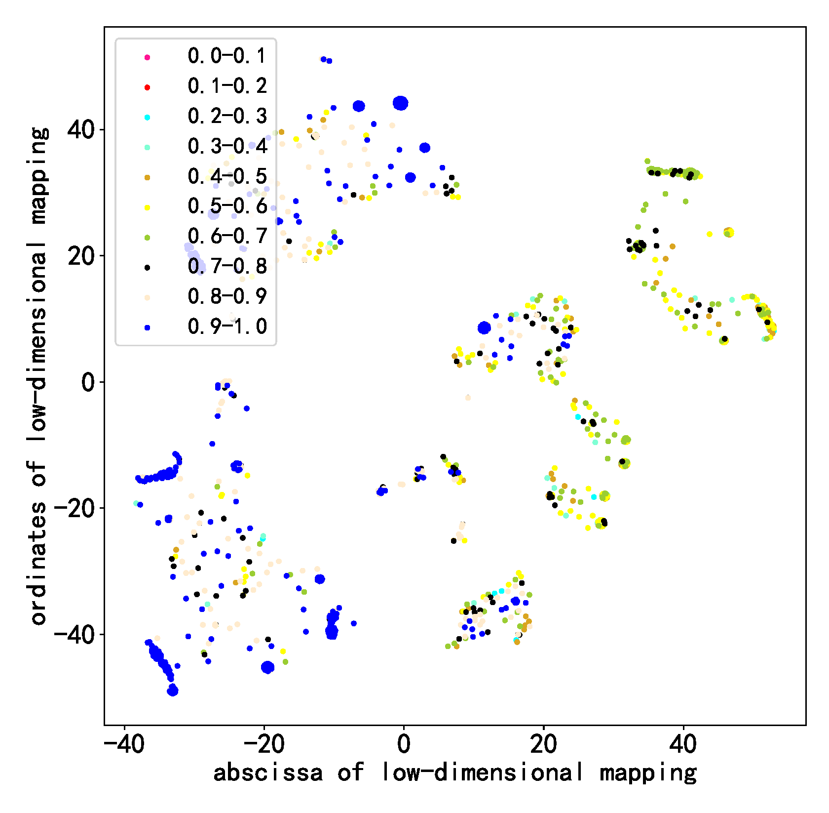
- After generating about 200,000 models, this paper analyzed the architecture of models with good performance and found that some combinations of architecture patterns frequently appeared in models with good performance. This paper conducted a t-SNE dimension reduction analysis on the model architecture sequences and found that the architecture sequences of models with good performance would also produce aggregation in the low-dimensional space; this shows that the models with good performance have some commonalities, and these results can provide a certain reference for future researchers in model design.
2. Previous Works
3. Methodology
3.1. Definition of Proposed Method
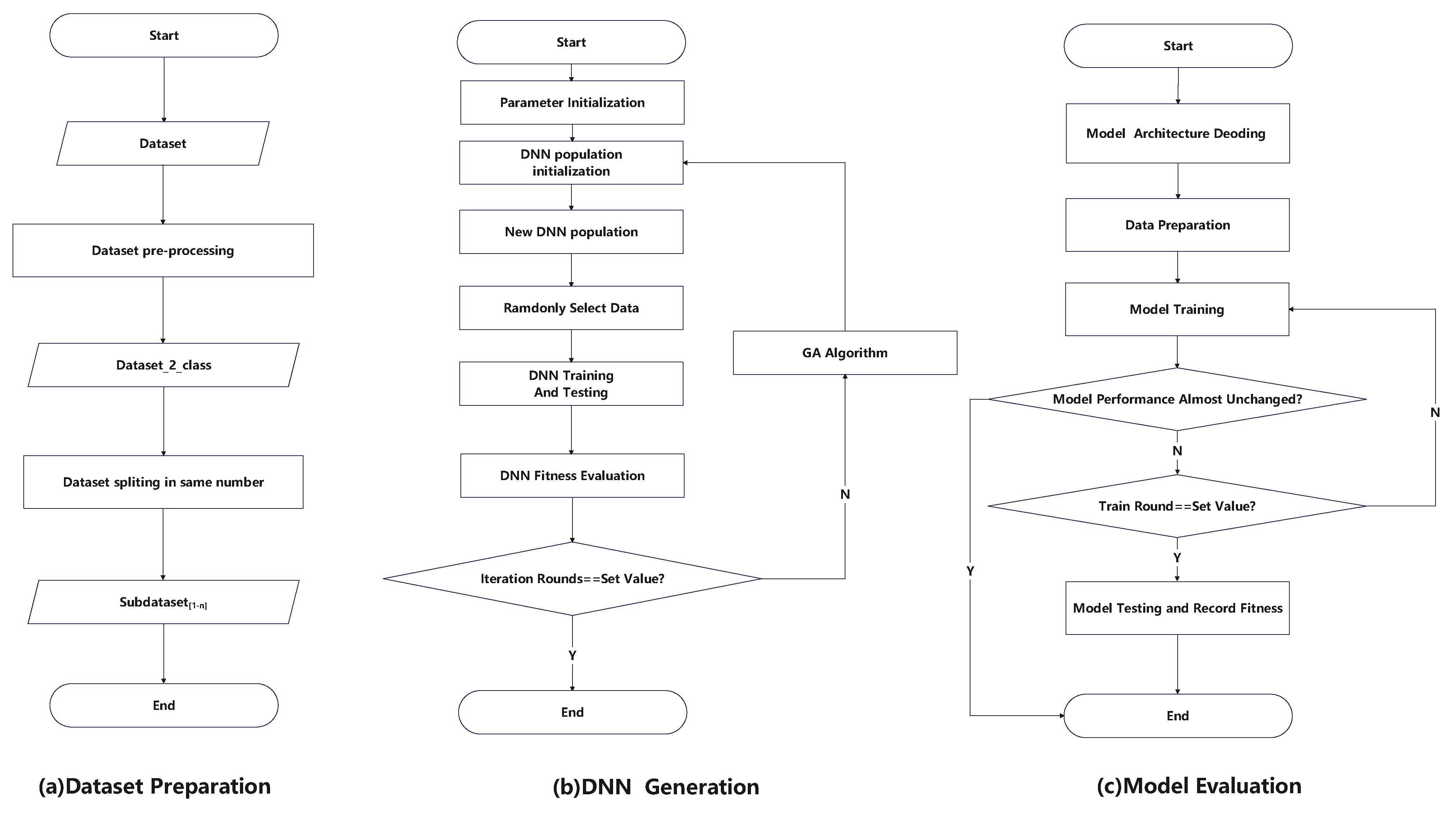
3.2. Dataset Preparation
3.3. Model Generation
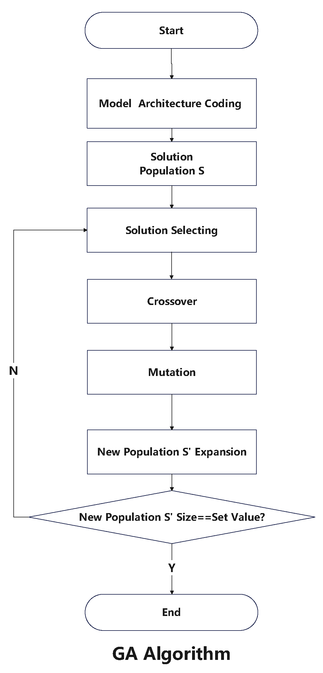
3.3.1. Introduction of the GA
- Selection: individuals in the population compete for survival resources, and the better individuals survive.
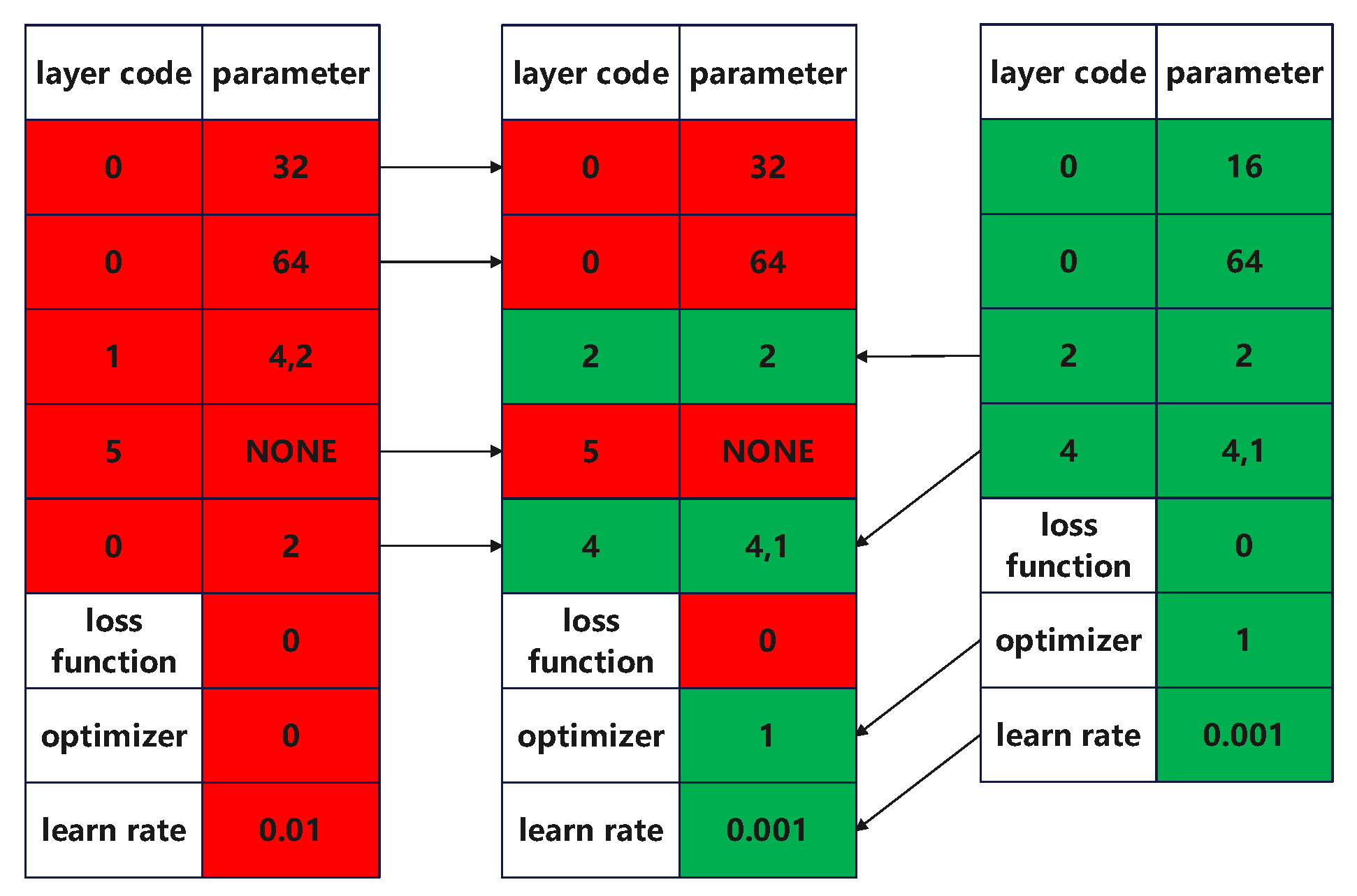
- Crossover: some characteristics of the previous generation can be passed on to the progeny so that the progeny and parents have a certain degree of similarity.
- Mutation: the newly generated individuals in the population will mutate, which leads to the introduction of some new characteristics in the population.
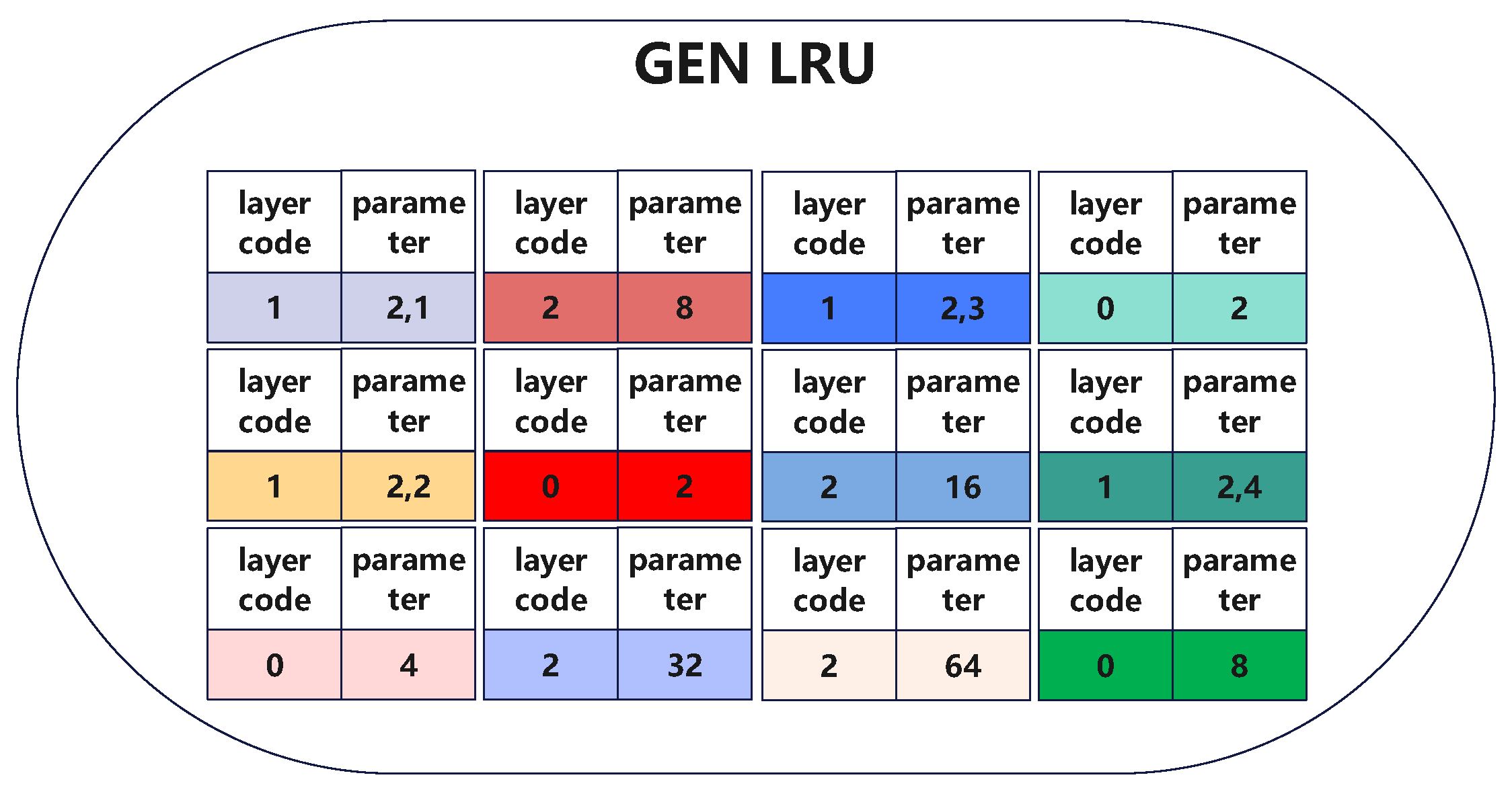
3.3.2. Coding Model Architecture
3.3.3. Fitness Function
3.3.4. Solution Selection
3.3.5. Crossover
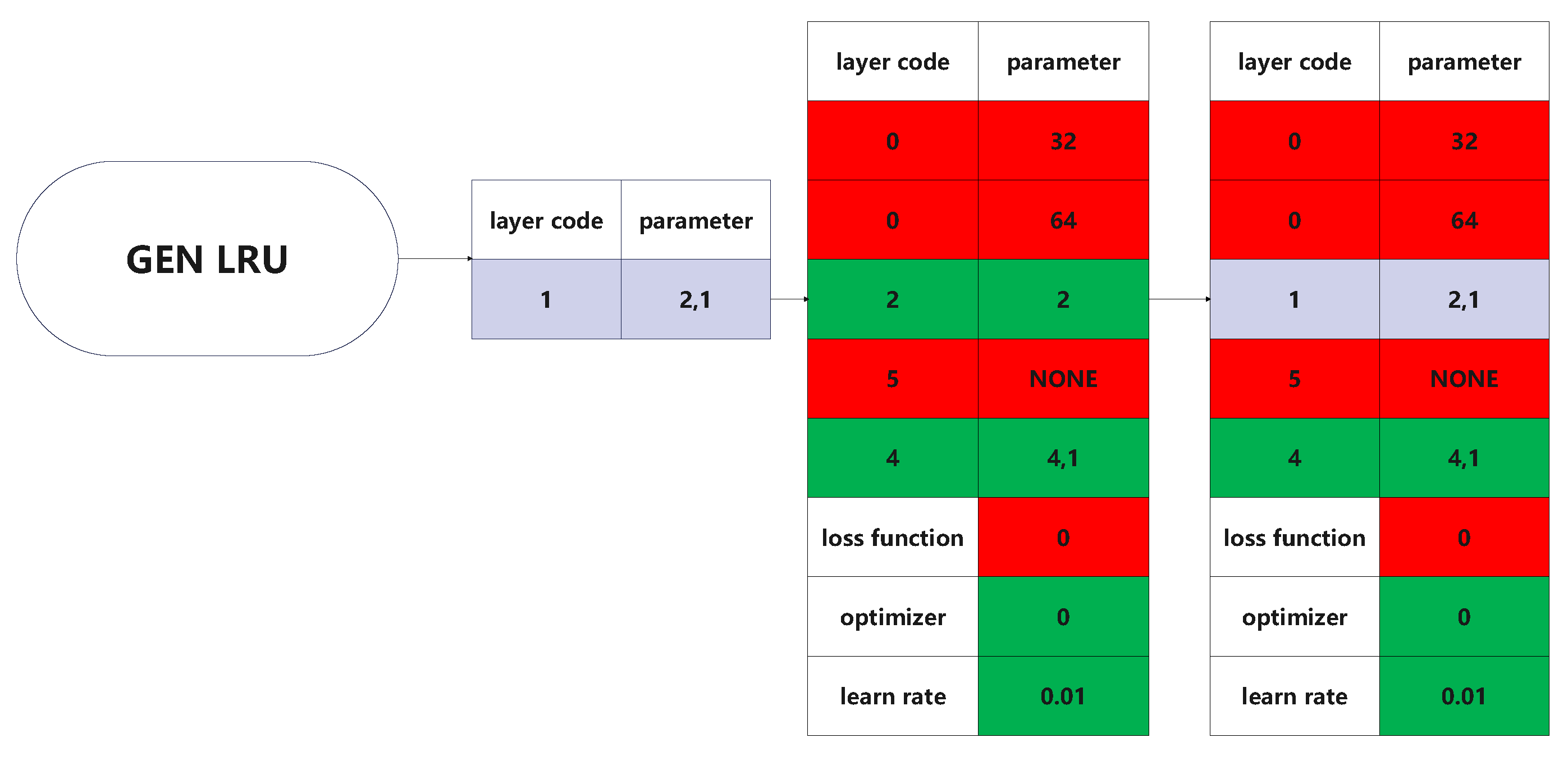
3.3.6. Mutation
3.4. Model Evaluation
4. Experiment and Evaluation
4.1. Dataset Selection
4.2. Data Preprocessing
- Remove invalid information from the input data: Some of the 87 features extracted by the CIC flowmeter tool should not be used as input features in the DNN. These are flow ID, time stamp, source IP, source port, target IP and target port. These features would all have different distributions in different application contexts and should not be taken as features to discern the abnormal flow of DDoS, which could otherwise cause overfitting problems in the DNN. Therefore, this paper removed these features in the data processing stage and chose other flow features as inputs to the DNN [43].
- Cleaning of datasets: This paper complemented the large number of NAN and INF in the raw data with the mean values of the other data.
- Transform labels in the manner of one-hot code: What was addressed in the experiment was a 2-Classification problem, so 1 × 2 one-hot coding was used to indicate the category of a piece of data [44].
- Data normalization processing: The normalization of the data can avoid numerically undesirable effects on the results because of the large difference in the orders of magnitude of the input data and is also convenient for the initialization of the DNN weights. Additionally, the data can be normalized to improve the speed of the gradient descent method for solving the optimal solution. This paper used the maximum–minimum Fmethod in the experiments to normalize the input data. The maximum–minimum method’s formula is as follows:where is the normalized data, X is the original data and and are the maximum and minimum values of the original dataset, respectively.
- Data expansion to solve the problem of uneven sample distribution: In the CICDDoS2019 dataset, there is a problem of an uneven distribution of sample data, in which the proportion of TFTP, SNMP and DNS traffic is significantly higher than other traffic. In the case of uneven data distribution in the dataset, the training and testing of the model are not objective [36,37,45]. In this paper, the dataset is expanded by the smote method. The smote method generates data through one piece of data and N pieces of data with the same category and the most similar features to avoid the over-fitting problem [46]. The formula generated by the smote method is as follows:where represents the expanded data, represents the original data in the dataset and represents a piece of data with the same category and similar features as . Table 5 shows the proportion of each type before and after smote method processing.
4.3. Evaluation
4.4. Hyperparameter Tuning
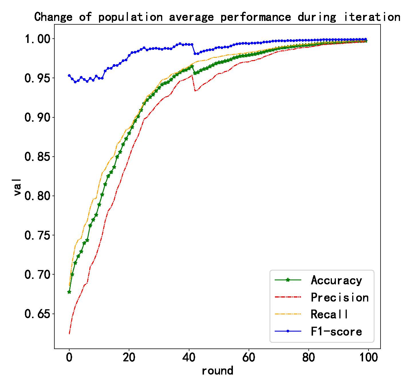
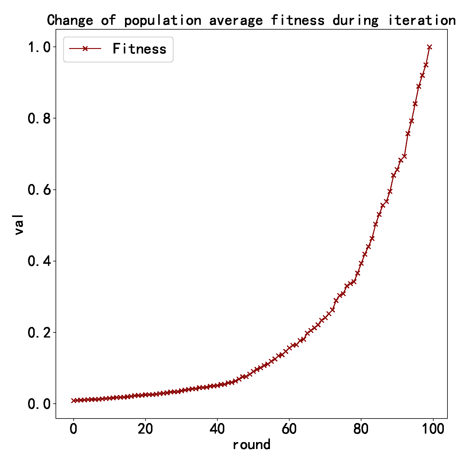
4.5. Model Generation
4.6. Evaluation of Models Generated
4.7. Comparative Experiment
5. Discussion
6. Conclusions and Future Work
Author Contributions
Funding
Institutional Review Board Statement
Informed Consent Statement
Data Availability Statement
Acknowledgments
Conflicts of Interest
References
- Sharifi, A.; Zad, F.F.; Farokhmanesh, F.; Noorollahi, A.; Sharif, J. An overview of intrusion detection and prevention systems (IDPS) and security issues. IOSR J. Comput. Eng. 2014, 16, 47–52. [Google Scholar] [CrossRef]
- Alshamrani, A.; Chowdhary, A.; Pisharody, S.; Lu, D.; Huang, D. A defense system for defeating DDoS attacks in SDN based networks. In Proceedings of the 15th ACM International Symposium on Mobility Management and Wireless Access, Miami, FL, USA, 21–25 November 2017; pp. 83–92. [Google Scholar]
- Bawany, N.Z.; Shamsi, J.A.; Salah, K. DDoS attack detection and mitigation using SDN: Methods, practices, and solutions. Arab. J. Sci. Eng. 2017, 42, 425–441. [Google Scholar] [CrossRef]
- Yaser, A.L.; Mousa, H.M.; Hussein, M. Improved DDoS Detection Utilizing Deep Neural Networks and Feedforward Neural Networks as Autoencoder. Future Internet 2022, 14, 240. [Google Scholar] [CrossRef]
- Thapa, N.; Liu, Z.; Kc, D.B.; Gokaraju, B.; Roy, K. Comparison of machine learning and deep learning models for network intrusion detection systems. Future Internet 2020, 12, 167. [Google Scholar] [CrossRef]
- Dong, S.; Abbas, K.; Jain, R. A survey on distributed denial of service (DDoS) attacks in SDN and cloud computing environments. IEEE Access 2019, 7, 80813–80828. [Google Scholar] [CrossRef]
- Sridaran, R. An Overview of DDoS Attacks in Cloud Environment. Available online: https://www.researchgate.net/profile/R-Sridaran/publication/273776292_An_Overview_of_DDoS_Attacks_in_Cloud_Environment/links/550d4d5e0cf275261098523d/An-Overview-of-DDoS-Attacks-in-Cloud-Environment.pdf (accessed on 25 November 2022).
- Swe, Y.M.; Aung, P.P.; Hlaing, A.S. A slow ddos attack detection mechanism using feature weighing and ranking. Int. Conf. Ind. Eng. Oper. Manag. 2021, 3, 4500–4509. [Google Scholar]
- Glorot, X.; Bengio, Y. Understanding the difficulty of training deep feedforward neural networks. In Proceedings of the Thirteenth International Conference on Artificial Intelligence and Statistics JMLR Workshop and Conference Proceedings, Chia Laguna Resort, Sardinia, Italy, 13–15 May 2010; pp. 249–256. [Google Scholar]
- Prasad, K.M.; Reddy, A.R.M.; Rao, K.V. DoS and DDoS attacks: Defense, detection and traceback mechanisms—A survey. Glob. J. Comput. Sci. Technol. 2014, 14, 15–32. [Google Scholar]
- Mohammed, S.S.; Hussain, R.; Senko, O.; Bimaganbetov, B.; Lee, J.; Hussain, F.; Kerrache, C.A.; Barka, E.; Bhuiyan, M.Z.A. A new machine learning-based collaborative DDoS mitigation mechanism in software-defined network. In Proceedings of the 14th International Conference on Wireless and Mobile Computing, Networking and Communications (WiMob), Limassol, Cyprus, 15–17 October 2018; pp. 1–8. [Google Scholar]
- Alotaibi, A.; Rassam, M.A. Adversarial Machine Learning Attacks against Intrusion Detection Systems: A Survey on Strategies and Defense. Future Internet 2023, 15, 62. [Google Scholar] [CrossRef]
- Said Elsayed, M.; Le-Khac, N.A.; Dev, S.; Jurcut, A.D. Machine-Learning Techniques for Detecting Attacks in SDN. arXiv 2019, arXiv:1910.00817. [Google Scholar]
- Zargar, S.T.; Joshi, J.; Tipper, D. A survey of defense mechanisms against distributed denial of service (DDoS) flooding attacks. IEEE Commun. Surv. Tutor. 2013, 15, 2046–2069. [Google Scholar] [CrossRef] [Green Version]
- Salim, M.M.; Rathore, S.; Park, J.H. Distributed denial of service attacks and its defenses in IoT: A survey. J. Supercomput. 2020, 76, 5320–5363. [Google Scholar] [CrossRef]
- Wang, H.; Li, W. DDosTC: A transformer-based network attack detection hybrid mechanism in SDN. Sensors 2021, 21, 5047. [Google Scholar] [CrossRef] [PubMed]
- Javeed, D.; Gao, T.; Khan, M.T. SDN-enabled hybrid DL-driven framework for the detection of emerging cyber threats in IoT. Electronics 2021, 10, 918. [Google Scholar] [CrossRef]
- Kreutz, D.; Ramos, F.M.V.; Verissimo, P. Towards secure and dependable software-defined networks. Second. Acm Sigcomm Workshop Hot Top. Softw. Defin. Netw. 2013, 8, 55–60. [Google Scholar]
- Alaoui, R.L.; Nfaoui, E.H. Deep learning for vulnerability and attack detection on web applications: A systematic literature review. Future Internet 2022, 14, 118. [Google Scholar] [CrossRef]
- Abdou, A.R.; Van Oorschot, P.C.; Wan, T. Comparative analysis of control plane security of SDN and conventional networks. IEEE Commun. Surv. Tutor. 2018, 20, 3542–3559. [Google Scholar] [CrossRef]
- Mattioli, F.; Caetano, D.; Cardoso, A.; Naves, E.; Lamounier, E. An experiment on the use of genetic algorithms for topology selection in deep learning. J. Electr. Comput. Eng. 2019, 2019, 3217542. [Google Scholar] [CrossRef] [Green Version]
- Xiao, X.; Yan, M.; Basodi, S.; Ji, C.; Pan, Y. Efficient hyperparameter optimization in deep learning using a variable length genetic algorithm. arXiv 2020, arXiv:2006.12703. [Google Scholar]
- Agrawal, A.; Singh, R.; Khari, M.; Vimal, S.; Lim, S. Autoencoder for design of mitigation model for DDOS attacks via M-DBNN. Wirel. Commun. Mob. Comput. 2022, 2022, 9855022. [Google Scholar] [CrossRef]
- Saha, S.; Sairam, A.S.; Yadav, A.; Ekbal, A. Genetic algorithm combined with support vector machine for building an intrusion detection system. In Proceedings of the International Conference on Advances in Computing, Communications and Informatics, Chennai, India, 3–5 August 2012; pp. 566–572. [Google Scholar]
- Kamel, H.; Abdullah, M.Z. Distributed denial of service attacks detection for software defined networks based on evolutionary decision tree model. Bull. Electr. Eng. Inform. 2022, 11, 2322–2330. [Google Scholar] [CrossRef]
- Erfan, A. DDoS attack detection scheme using hybrid ensemble learning and GA for internet of things. Palarch’S J. Archaeol. Egypt/Egyptol. 2021, 18, 521–546. [Google Scholar]
- Chiba, Z.; Abghour, N.; Moussaid, K.; El Omri, A.; Rida, M. Smart approach to build a deep neural network based ids for cloud environment using an optimized genetic algorithm. In Proceedings of the 2nd International Conference on Networking, Information Systems & Security, Rabat, Morocoo, 27–28 March 2019; 1–12. [Google Scholar]
- Zainudin, A.; Ahakonye, L.A.C.; Akter, R.; Kim, D.S.; Lee, J.M. An efficient hybrid-dnn for ddos detection and classification in software-defined iiot networks. IEEE Internet Things J. 2022. [Google Scholar] [CrossRef]
- Sindian, S.; Samer, S. An enhanced deep autoencoder-based approach for DDoS attack detection. Wseas Trans. Syst. Control 2020, 15, 716–725. [Google Scholar] [CrossRef]
- Kunang, Y.N.; Nurmaini, S.; Stiawan, D.; Suprapto, B.Y. Attack classification of an intrusion detection system using deep learning and hyperparameter optimization. J. Inf. Secur. Appl. 2021, 58, 102804. [Google Scholar] [CrossRef]
- Huang, S.; Li, X.; Cheng, Z.; Zhang, Z.; Hauptmann, A. Gnas: A greedy neural architecture search method for multi-attribute learning. arXiv 2018, arXiv:abs/1804.06964. [Google Scholar]
- Bergstra, J.; Bengio, Y. Random search for hyper-parameter optimization. J. Mach. Learn. Res. 2012, 13, 281–305. [Google Scholar]
- Aamir, M.; Zaidi, S.M.A. DDoS attack detection with feature engineering and machine learning: The framework and performance evaluation. Int. J. Inf. Secur. 2019, 18, 761–785. [Google Scholar] [CrossRef]
- Jordan, M.I.; Mitchell, T.M. Machine learning: Trends, perspectives, and prospects. Science 2015, 349, 255–260. [Google Scholar] [CrossRef]
- Shafique, M.; Hafiz, R.; Javed, M.U.; Abbas, S.; Sekanina, L.; Vasicek, Z.; Mrazek, V. Adaptive and energy-efficient architectures for machine learning: Challenges, opportunities, and research roadmap. In Proceedings of the 2017 IEEE Computer society annual symposium on VLSI (ISVLSI), Bochum, Germany, 3–5 July 2017; pp. 627–632. [Google Scholar]
- Huang, C.; Li, Y.; Loy, C.C.; Tang, X. Learning deep representation for imbalanced classification. In Proceedings of the IEEE Conference on Computer Vision and Pattern Recognition, Las Vegas, NV, USA, 27–30 June 2016; pp. 5375–5384. [Google Scholar]
- Johnson, J.M.; Khoshgoftaar, T.M. Survey on deep learning with class imbalance. J. Big Data 2019, 6, 27. [Google Scholar] [CrossRef] [Green Version]
- Pandey, H.M.; Chaudhary, A.; Mehrotra, D. A comparative review of approaches to prevent premature convergence in GA. Appl. Soft Comput. 2014, 24, 1047–1077. [Google Scholar] [CrossRef]
- Mathew, T.V. Genetic Algorithm. Report Submitted at IIT Bombay. 2012. Available online: http://datajobstest.com/data-science-repo/Genetic-Algorithm-Guide-[Tom-Mathew].pdf (accessed on 18 November 2022).
- Pham, T.A.; Tran, V.Q.; Vu, H.L.T.; Ly, H.B. Design deep neural network architecture using a genetic algorithm for estimation of pile bearing capacity. PLoS ONE 2020, 15, e0243030. [Google Scholar] [CrossRef]
- Katoch, S.; Chauhan, S.S.; Kumar, V. A review on genetic algorithm: Past, present, and future. Multimed. Tools Appl. 2021, 80, 8091–8126. [Google Scholar]
- Ring, M.; Wunderlich, S.; Scheuring, D.; Landes, D.; Hotho, A. A survey of network-based intrusion detection data sets. Comput. Secur. 2019, 86, 147–167. [Google Scholar] [CrossRef] [Green Version]
- Yang, J.; Zhao, Y.-Q.; Chan, J.C.-W. Learning andtransferring deep joint spectral-spatial features for hyper-spectral classification. IEEE Trans. Geosci. Remote Sens. 2017, 55, 4729–4742. [Google Scholar] [CrossRef]
- Jie, L.; Jiahao, C.; Xueqin, Z.; Yue, Z.H.O.U.; Jiajun, L.I.N. One-hot encoding and convolutional neural network based anomaly detection. J. Tsinghua Univ. (Sci. Technol.) 2019, 59, 523–529. [Google Scholar]
- Srivastava, N.; Hinton, G.; Krizhevsky, A.; Sutskever, I.; Salakhutdinov, R. Dropout: A simple way to prevent neural networks from overfitting. J. Mach. Learn. Res. 2014, 15, 1929–1958. [Google Scholar]
- Chawla, N.V.; Bowyer, K.W.; Hall, L.O.; Kegelmeyer, W.P. SMOTE: Synthetic minority over-sampling technique. J. Artif. Intell. Res. 2002, 16, 321–357. [Google Scholar] [CrossRef]
- Elsayed, M.S.; Le-Khac, N.A.; Dev, S.; Jurcut, A.D. Ddosnet: A deep-learning model for detecting network attacks. In Proceedings of the 2020 IEEE 21st International Symposium on “A World of Wireless, Mobile and Multimedia Networks” (WoWMoM), Cork, Ireland, 31 August–3 September 2020; pp. 391–396. [Google Scholar]
- Chartuni, A.; Márquez, J. Multi-Classifier of DDoS Attacks in Computer Networks Built on Neural Networks. Appl. Sci. 2021, 11, 10609. [Google Scholar] [CrossRef]
- Cil, A.E.; Yildiz, K.; Buldu, A. Detection of DDoS attacks with feed forward based deep neural network model. Expert Syst. Appl. 2021, 169, 114520. [Google Scholar] [CrossRef]
- Mahadik, S.S.; Pawar, P.; Muthalagu, R. Edge-HetIoT Defense against DDoS Attack Using LearningTechniques. 2022. Available online: https://assets.researchsquare.com/files/rs-2164979/v1_covered.pdf?c=1668326371 (accessed on 18 November 2022).
- Rangapur, A.; Kanakam, T.; Jubilson, A. DDoSDet: An approach to Detect DDoS attacks using Neural Networks. arXiv 2022, arXiv:2201.09514. [Google Scholar]


| Symbol | Description |
|---|---|
| P | Set of solutions |
| A solution in the population, the subscript id represents the id number of the solution | |
| The probability that a solution is selected to participate in generating a new solution | |
| The length of a sequence corresponding to a solution | |
| F | Set of fitness of solutions |
| Weight of accuracy in fitness function | |
| Weight of single data processing time in fitness function | |
| Represents the average time of processing a single piece of data in the test phase of the model | |
| The fitness value of a solution | |
| [,] | The corresponding cumulative probability interval of the solution |
| The probability that a solution is selected to provide a gene fragment to a new solution | |
| A random number | |
| A value used to determine whether to use GEN LRU |
| Description | Code | Parameter |
|---|---|---|
| Full Connected Layer | 0 | Neurons {2,4,6,8,16,32,64} |
| Conv2d | 1 | Kernel size {2,4,6,8} Stride {1,2,3,4} |
| Maxpool2d | 2 | Pooling {2,3,4,5} |
| Droupout | 3 | Dropout rate {0.1,0.2,0.3,0.4,0.5} |
| Residual layer | 4 | Kernel size {2,4,6,8} Padding {1,2,3,4} |
| Activation Functions | Code | Optimizer | Code | Loss Function | Code |
|---|---|---|---|---|---|
| Relu | 5 | Adam | 0 | Logarithmic Cross Entropy Loss | 0 |
| Sigmoid | 6 | Sgd | 1 | Mse Loss | 1 |
| Tanh | 7 | Rmdgrop | 2 | Smooth Mse Loss | 2 |
| Softplus | 8 | L1 Loss | 3 |
| Description | Code | Parameter |
|---|---|---|
| Full Connection Layer with 32 neurons | 0 | 32 |
| Full Connection Layer with 64 neurons | 0 | 64 |
| Conv2d with 4∗4 Convolutional filter and stride is 2 | 1 | 4,2 |
| Relu activation | 5 | |
| Full Connected Layer with 2 neurons | 0 | 2 |
| Logarithmic cross entropy loss | 0 | |
| Adam optimizer | 0 | |
| Learn Rate | 0.01 |
| Tag | Percentage before Smote Method | Percentage after Smote Method |
|---|---|---|
| BENIGN | 0.00114 | 0.05011 |
| DrDoS_DNS | 0.10129 | 0.08262 |
| DrDoS_NetBIOS | 0.08176 | 0.08309 |
| DrDoS_NTP | 0.02402 | 0.07811 |
| UDP-lag | 0.00732 | 0.08163 |
| WebDDoS | 0.00001 | 0.04184 |
| DrDoS_UDP | 0.06261 | 0.08296 |
| DrDoS_MSSQL | 0.09034 | 0.08306 |
| Syn | 0.03161 | 0.08333 |
| DrDoS_LDAP | 0.04354 | 0.08332 |
| DrDoS_SSDP | 0.05215 | 0.08329 |
| TFTP | 0.40115 | 0.08333 |
| DrDoS_SNMP | 0.10307 | 0.08332 |
| Method | ACC | PRE | REC | F1_SCORE |
|---|---|---|---|---|
| (50,400) | 0.9913 | 0.9978 | 0.9848 | 0.9913 |
| (100,200) | 0.9913 | 0.9975 | 0.9850 | 0.9912 |
| (200,100) | 0.9937 | 0.9996 | 0.9878 | 0.9937 |
| (400,50) | 0.9909 | 0.9974 | 0.9844 | 0.9909 |
| Complexity Cost | Range |
|---|---|
| Flops (M) | [0.01,6.1] |
| Pamras (M) | [0.0,0.01] |
| Complexity Cost | Average Value |
|---|---|
| Flops (M) | 0.1105 |
| Pamras (M) | 0.0020 |
| Normal | Attack | |
|---|---|---|
| Normal | 0.9994 | 0.0006 |
| Attack | 0.0119 | 0.9881 |
| Techniques | ACC | PRE | REC | F1_SCORE |
|---|---|---|---|---|
| Best model generated | 0.9937 | 0.9993 | 0.9881 | 0.9937 |
| Mahmoud Said Elsayed et al. [47] | 0.9913 | 0.9990 | 0.9837 | 0.9913 |
| Andrés Chartuni et al. [48] | 0.9927 | 0.9999 | 0.9855 | 0.9927 |
| Abdullah Emir Cil et al. [49] | 0.9914 | 0.9985 | 0.9846 | 0.9915 |
| Shalaka S. Mahadik et al. [50] | 0.9866 | 0.9964 | 0.9771 | 0.9867 |
| Aman Rangapur et al. [51] | 0.9921 | 0.9987 | 0.9857 | 0.9921 |
| SVM | 0.8024 | 0.9646 | 0.6243 | 0.7580 |
| C4.5 | 0.9817 | 0.9795 | 0.9840 | 0.9817 |
| RF | 0.7862 | 0.9931 | 0.5800 | 0.7323 |
| LR | 0.5071 | 0.5071 | 1.0000 | 0.6729 |
| Dataset | ACC | PRE | REC | F1_SCORE |
|---|---|---|---|---|
| CICIDS2017 | 0.9906 | 0.9896 | 0.9915 | 0.9906 |
| CICIDS2018 | 0.9993 | 0.9986 | 1.0000 | 0.9993 |
| Method | Flops (M) | Params (M) |
|---|---|---|
| Model generation using six datasets | 0.2173 | 0.0038 |
| Model generation using one dataset | 0.1105 | 0.0020 |
| Chiba Z et al. [27] | 0.9507 | 0.0305 |
| Techniques | ACC | PRE | REC | F1_SCORE | T (ms) | KS |
|---|---|---|---|---|---|---|
| Best model generated with six datasets | 0.9902 | 0.9903 | 0.9903 | 0.9902 | 0.001477 | 0.607 |
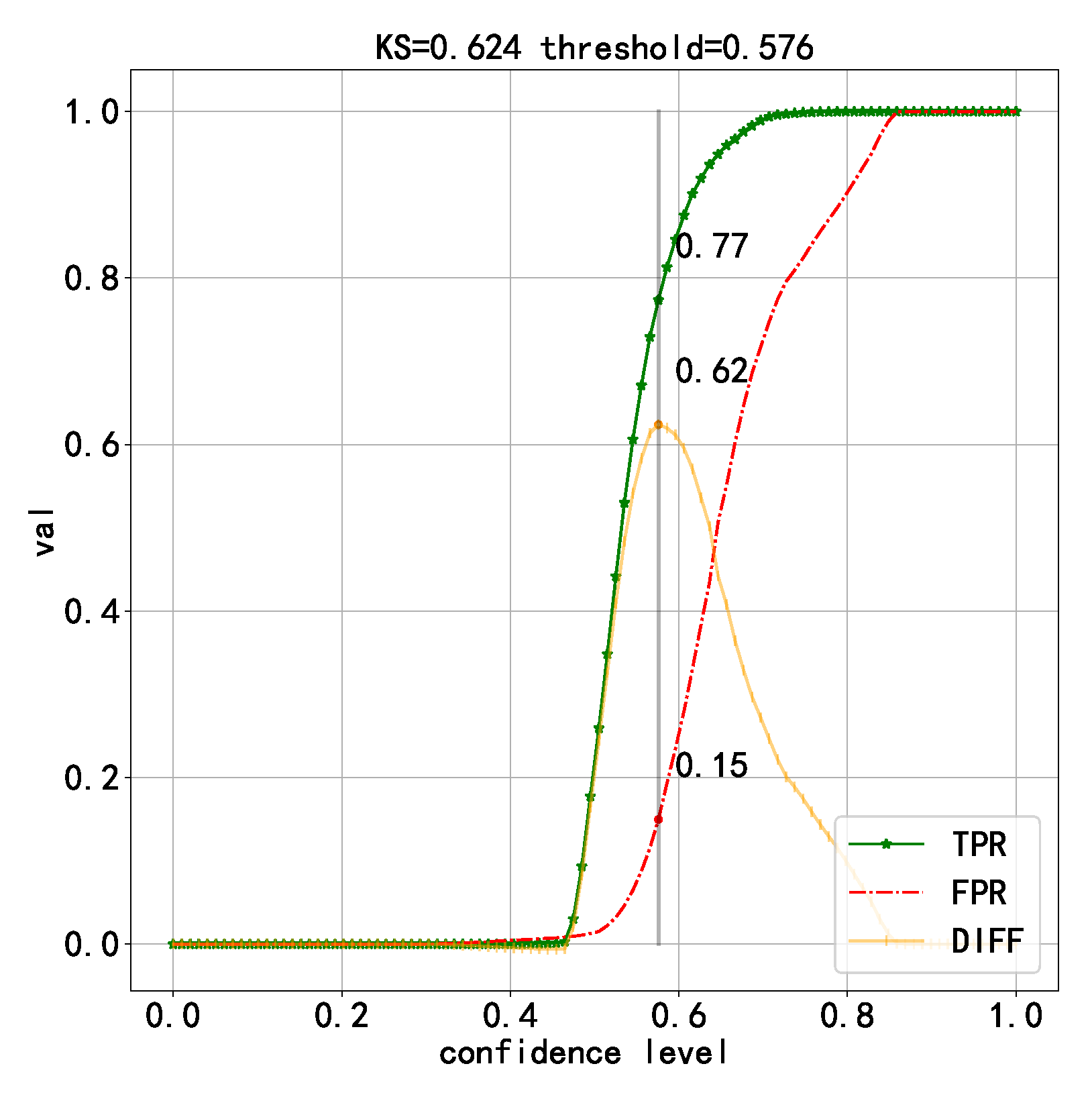
| Best model generated with one dataset | 0.9937 | 0.9993 | 0.9881 | 0.9937 | 0.001340 | 0.624 |
| Best model generated by Chiba Z et al. [27] | 0.9777 | 0.9785 | 0.9778 | 0.9777 | 0.001371 | 0.605 |
| Techniques | Dataset | ACC | PRE | REC | F1_SCORE |
|---|---|---|---|---|---|
| Best model generated with six datasets | CICDDoS2019 | 0.9902 | 0.9903 | 0.9903 | 0.9902 |
| CICIDS2017 | 0.9660 | 0.9664 | 0.9660 | 0.9660 | |
| CICIDS2018 | 0.9984 | 0.9984 | 0.9984 | 0.9984 | |
| KDD_CUP99 | 1.0000 | 1.0000 | 1.0000 | 1.00000 | |
| NSL-KDD | 0.9352 | 0.9354 | 0.9352 | 0.9352 | |
| UNSW | 1.0000 | 1.0000 | 1.0000 | 1.0000 | |
| Best model generated with one dataset | CICDDoS2019 | 0.9937 | 0.9993 | 0.9881 | 0.9937 |
| CICIDS2017 | 0.7460 | 0.7500 | 0.7458 | 0.7449 | |
| CICIDS2018 | 0.5029 | 0.7514 | 0.5000 | 0.3346 | |
| KDD_CUP99 | 0.9079 | 0.9225 | 0.9076 | 0.9071 | |
| NSL-KDD | 0.7675 | 0.7795 | 0.7663 | 0.7644 | |
| UNSW | 0.4817 | 0.4649 | 0.4835 | 0.4039 | |
| Best model generated by Chiba Z et al. [27] | CICDDoS2019 | 0.9777 | 0.9785 | 0.9778 | 0.9777 |
| CICIDS2017 | 0.8121 | 0.8202 | 0.8117 | 0.8108 | |
| CICIDS2018 | 0.6591 | 0.6879 | 0.6583 | 0.6448 | |
| KDD_CUP99 | 0.9995 | 0.9995 | 0.9995 | 0.9995 | |
| NSL-KDD | 0.7010 | 0.7018 | 0.7012 | 0.7010 | |
| UNSW | 0.4937 | 0.4968 | 0.4999 | 0.3308 |
| Topology Layer | Percentage of Occurrence |
|---|---|
| Full Connected Layer | 0.2597 |
| Conv2d | 0.0175 |
| Maxpool2d | 0.0957 |
| Droupout | 0.0087 |
| Residual layer | 0.1693 |
| Relu | 0.0896 |
| Sigmoid | 0.0412 |
| Tanh | 0.0773 |
| Softplus | 0.2402 |
| Number of Occurrences | 1 | 2 | 3 | 4 |
|---|---|---|---|---|
| Full Connected Layer | 0.5050 | 0.3110 | 0.1220 | 0.0470 |
| Conv2d | 0.8100 | 0.1800 | 0.0000 | 0.0000 |
| Maxpool2d | 0.2380 | 0.6875 | 0.0588 | 0.0147 |
| Droupout | 0.9705 | 0.0294 | 0.0000 | 0.0000 |
| Residual layer | 0.3375 | 0.4936 | 0.1278 | 0.0358 |
| Relu | 0.6000 | 0.2923 | 0.0769 | 0.0307 |
| Sigmoid | 0.6825 | 0.0950 | 0.0222 | 0.0000 |
| Tanh | 0.2463 | 0.6811 | 0.0724 | 0.0000 |
| Softplus | 0.3913 | 0.4434 | 0.1217 | 0.0347 |
Disclaimer/Publisher’s Note: The statements, opinions and data contained in all publications are solely those of the individual author(s) and contributor(s) and not of MDPI and/or the editor(s). MDPI and/or the editor(s) disclaim responsibility for any injury to people or property resulting from any ideas, methods, instructions or products referred to in the content. |
© 2023 by the authors. Licensee MDPI, Basel, Switzerland. This article is an open access article distributed under the terms and conditions of the Creative Commons Attribution (CC BY) license (https://creativecommons.org/licenses/by/4.0/).
Share and Cite
Zhao, J.; Xu, M.; Chen, Y.; Xu, G. A DNN Architecture Generation Method for DDoS Detection via Genetic Alogrithm. Future Internet 2023, 15, 122. https://doi.org/10.3390/fi15040122
Zhao J, Xu M, Chen Y, Xu G. A DNN Architecture Generation Method for DDoS Detection via Genetic Alogrithm. Future Internet. 2023; 15(4):122. https://doi.org/10.3390/fi15040122
Chicago/Turabian StyleZhao, Jiaqi, Ming Xu, Yunzhi Chen, and Guoliang Xu. 2023. "A DNN Architecture Generation Method for DDoS Detection via Genetic Alogrithm" Future Internet 15, no. 4: 122. https://doi.org/10.3390/fi15040122