
On the Use of Knowledge Transfer Techniques for Biomedical Named Entity Recognition †

Abstract
:1. Introduction
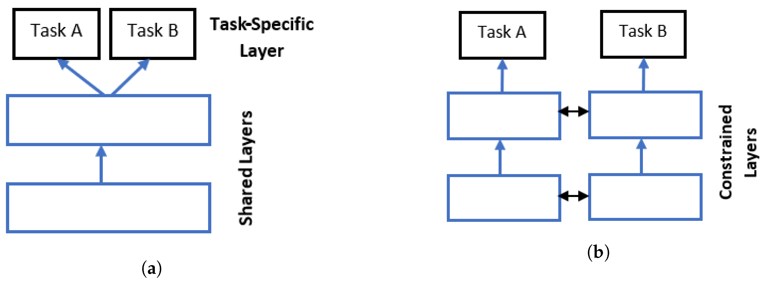
1.1. Multitask Learning
1.2. Transfer Learning
2. Proposed Methods
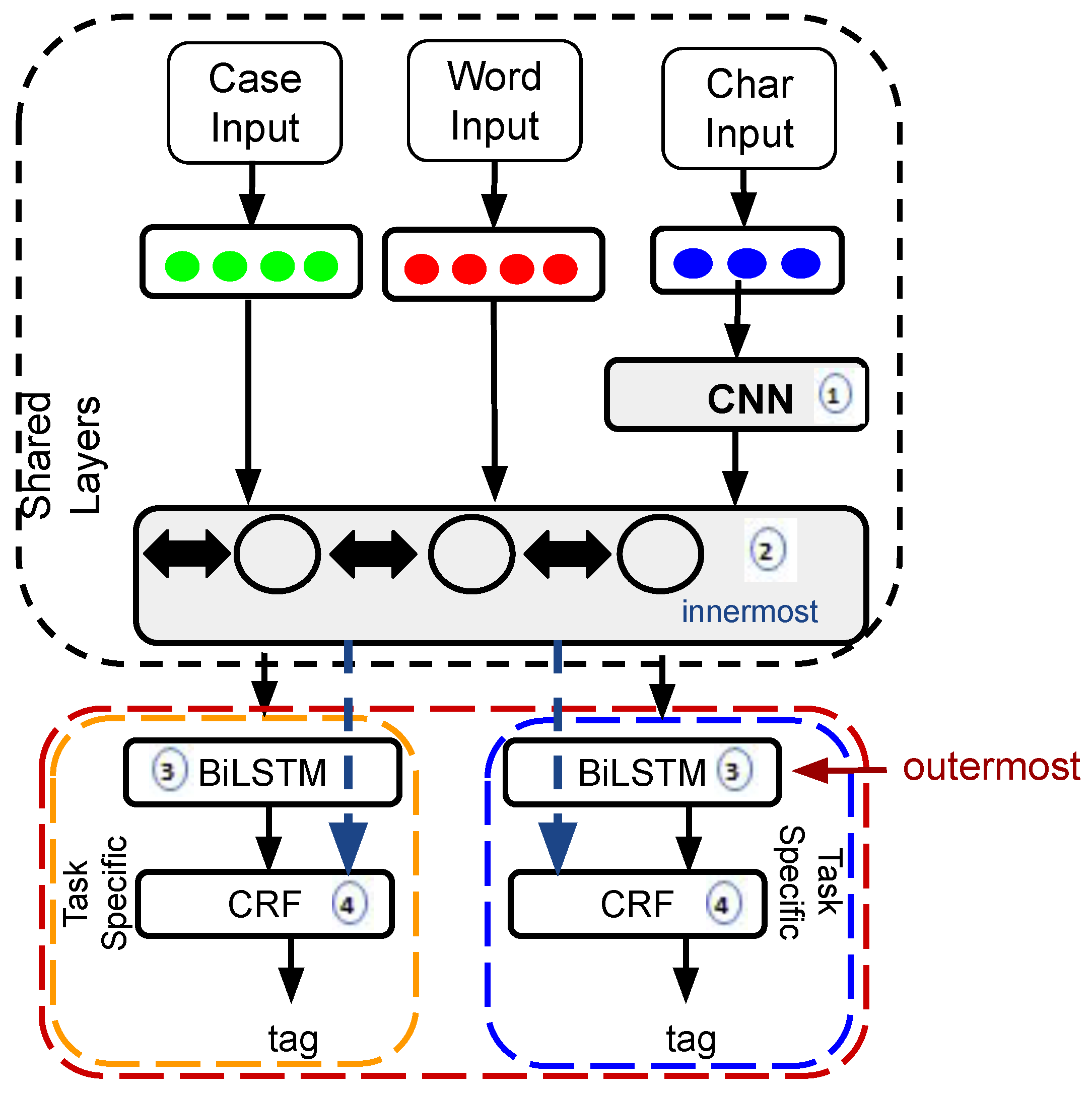
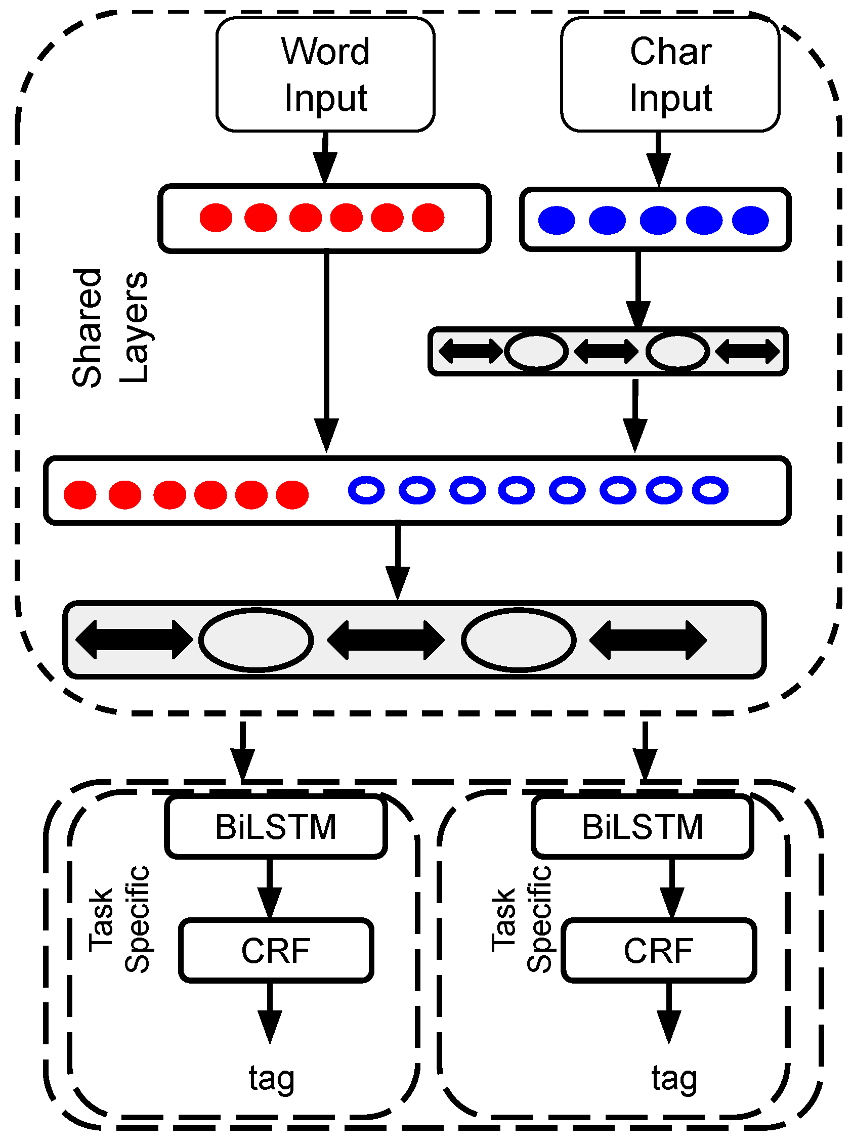
2.1. MTM-CNN Model
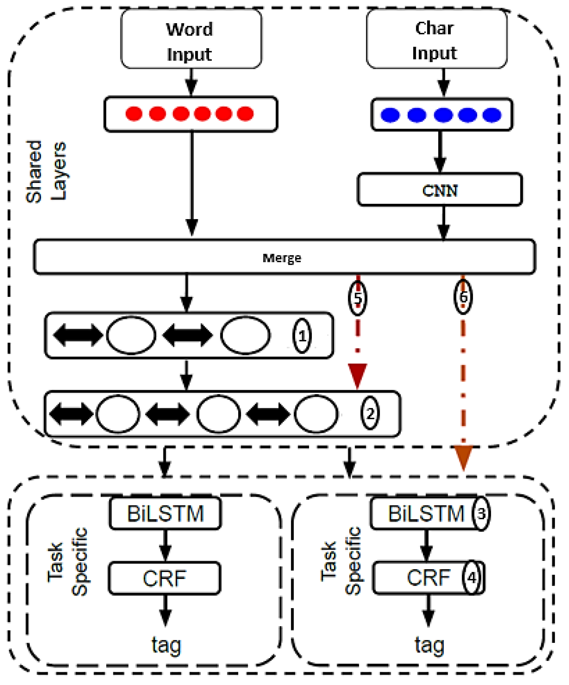
2.2. MTM-CW Model
2.3. Multi-Task Model with Transfer Learning
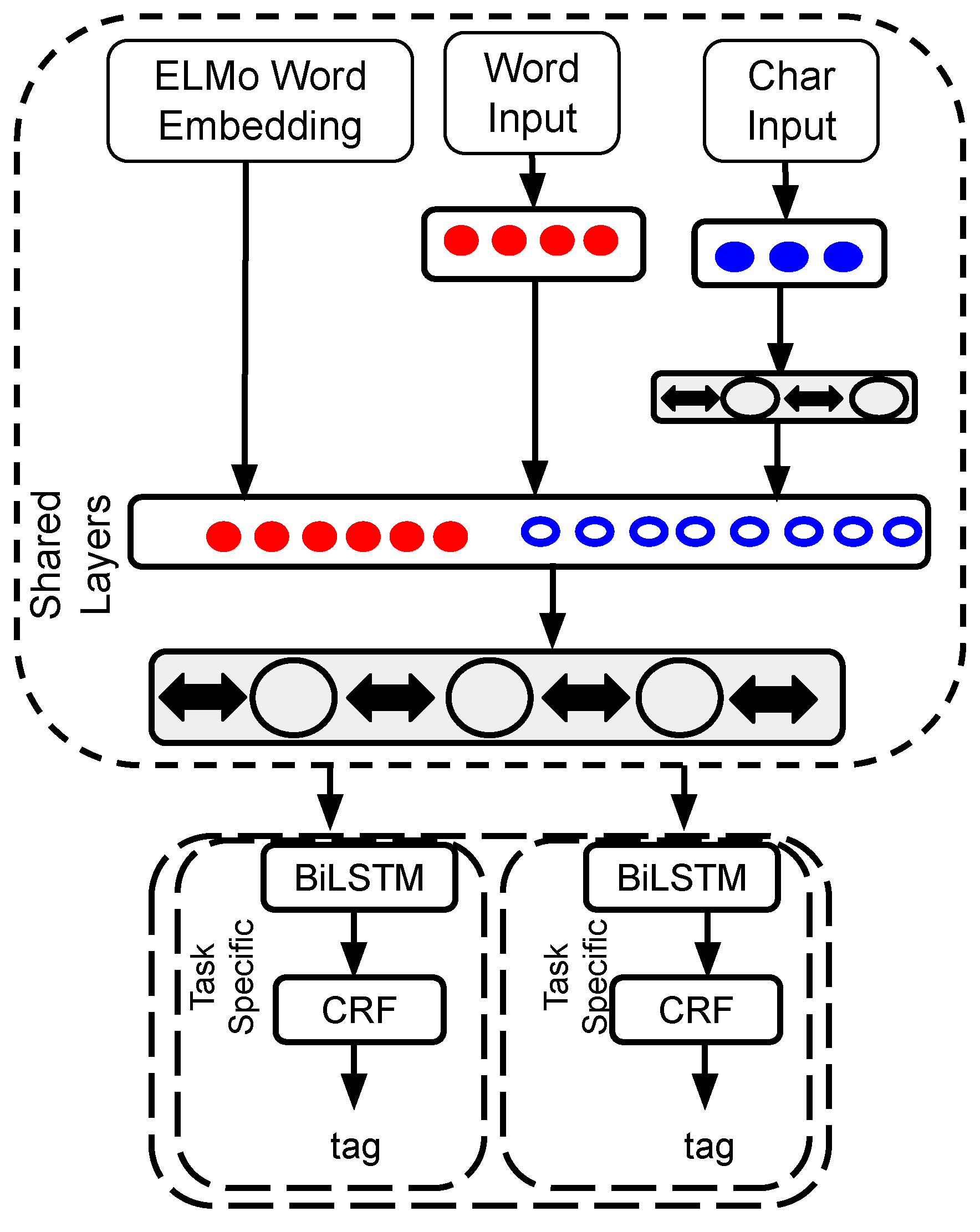
2.4. Embeddings from Language Models
3. Experiments
4. Results and Discussion of MTM-CNN
4.1. Effects of Different Auxiliary Tasks
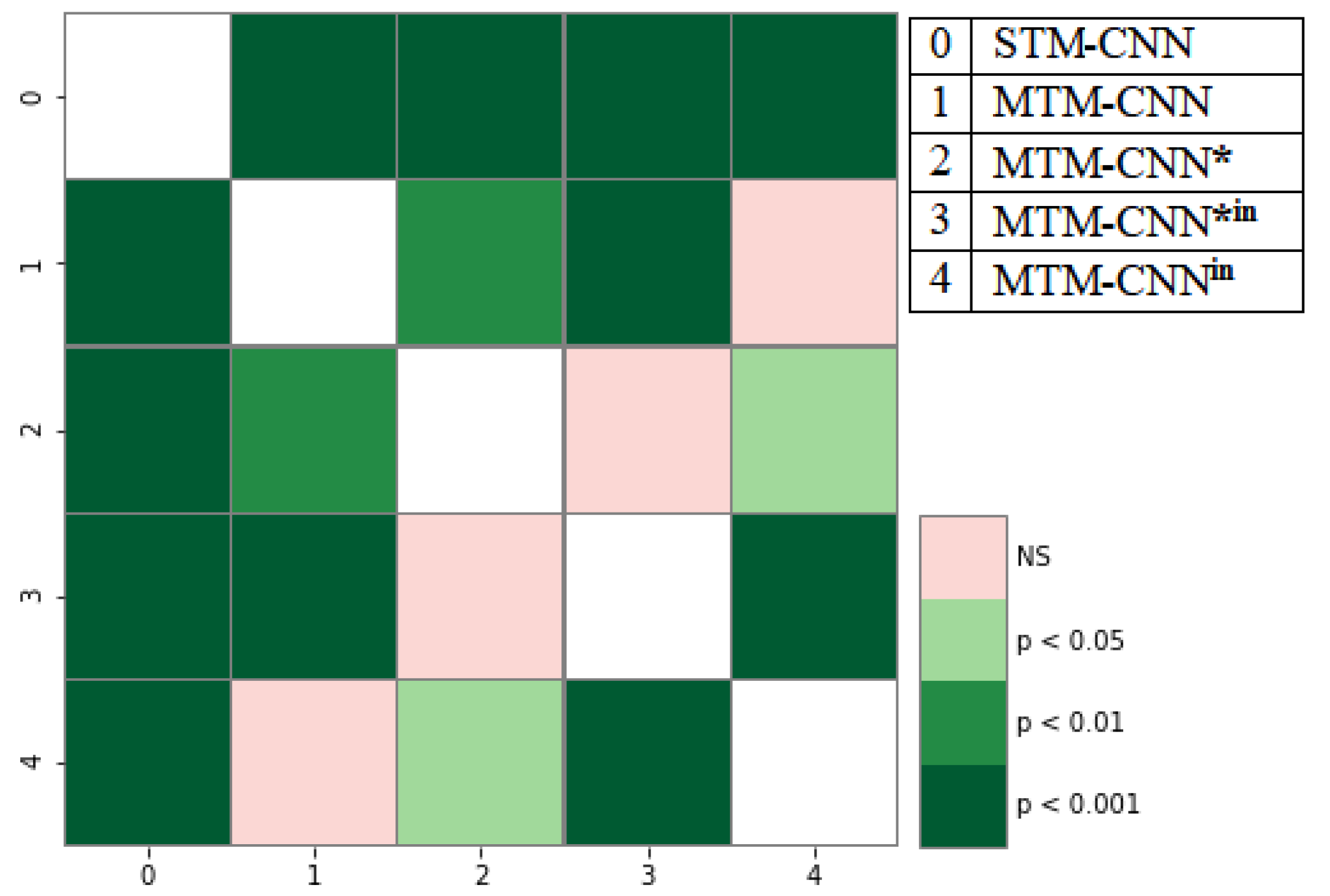
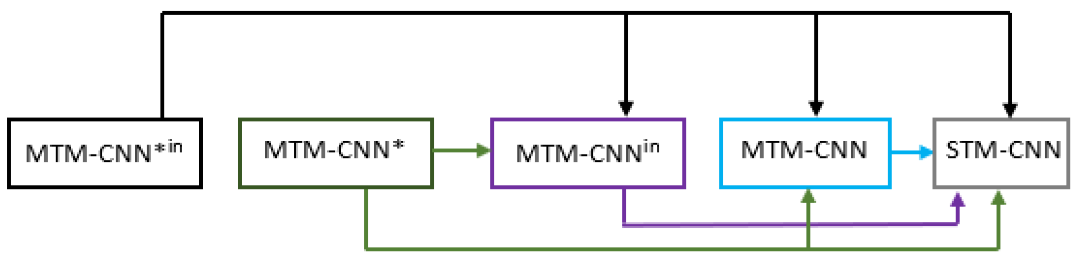
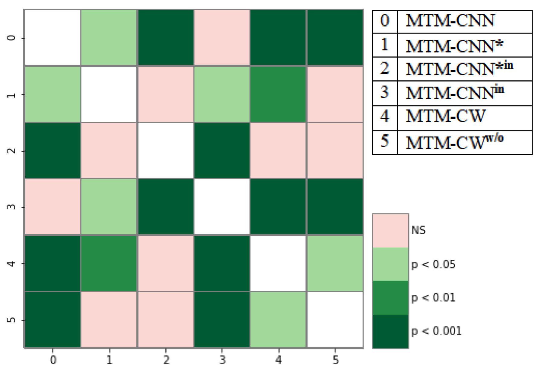
4.2. Statistical Analysis of MTM-CNN
5. Results and Discussion of MTM-CW
Statistical Analysis of MTM-CW
6. Results and Discussion for Fine-Tuned MTM ()
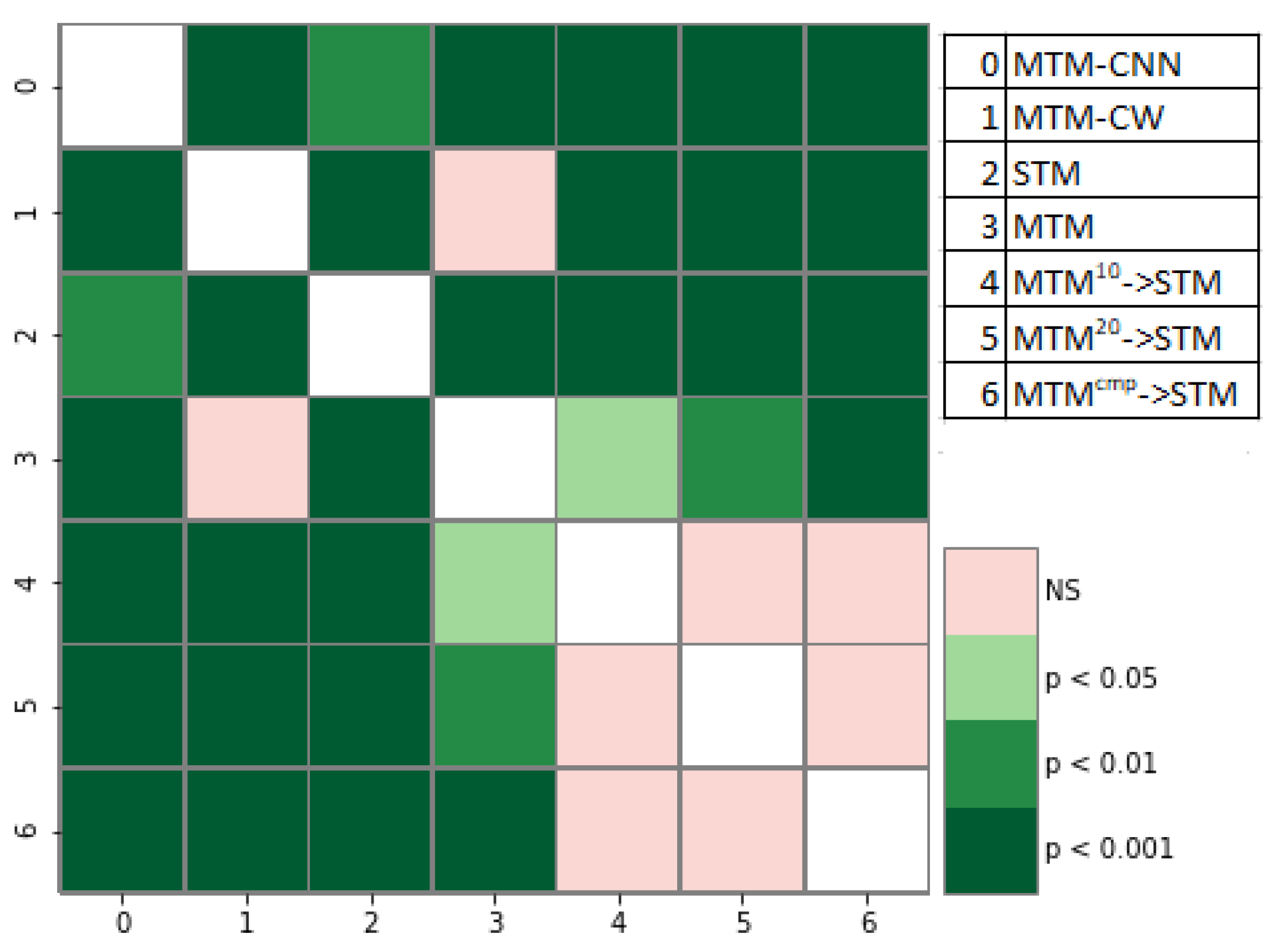
Statistical Analysis of
7. Results and Discussion for ELMo
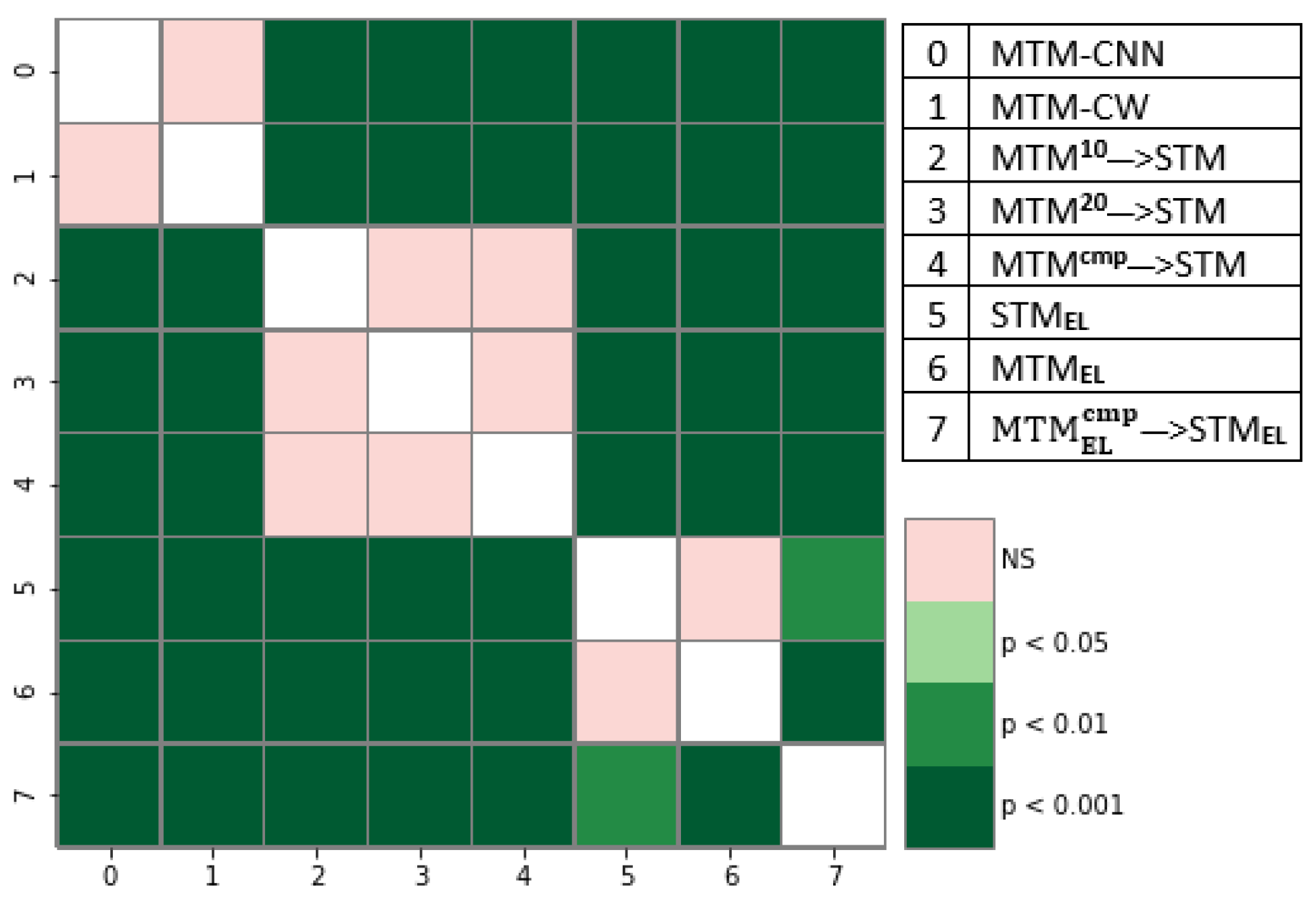
Statistical Analysis of ELMo
8. Conclusions
Author Contributions
Funding
Data Availability Statement
Conflicts of Interest
Appendix A. Datasets
Appendix A.1. AnatEM
Appendix A.2. BC2GM
Appendix A.3. BC4CHEMD
Appendix A.4. BC5CDR

| Dataset | Contents | Entity Counts |
|---|---|---|
| AnatEM | Anatomy NE | 13,701 |
| BC2GM | Gene/protein NE | 24,583 |
| BC4CHEMD | Chemical NE | 84,310 |
| BC5CDR | Chemical, disease NEs | Chemical: 15,935; disease: 12,852 |
| BioNLP09 | Gene/protein NE | 14,963 |
| BioNLP11EPI | Gene/protein NE | 15,811 |
| BioNLP11ID | 4 NEs | Gene/protein: 6551; organism: 3471 chemical: 973; regulon-operon: 87 |
| BioNLP13CG | 16 NEs | Gene/protein: 7908; cell: 3492; chemical: 2270; organism: 1715; tissue: 587; multitissue structure: 857; amino acid: 135; cellular component: 569; organism substance: 283; organ: 421; pathological formation: 228; immaterial anatomical entity: 102; organism subdivision: 98; anatomical system: 41; cancer: 2582; developing anatomical structure: 35 |
| BioNLP13GE | Gene/protein NE | 12,057 |
| BioNLP13PC | 4 NEs | Gene/protein: 10,891; chemical: 2487; complex: 1502; cellular component: 1013 |
| CRAFT | 6 NEs | SO: 18,974; gene/protein: 16,064; cl: 5495; taxonomy: 6868; chemical: 6053; GO-CC: 4180 |
| Ex-PTM | Gene/protein NE | 4698 |
| JNLPBA | 5 NEs | Gene/protein: 35,336; DNA: 10,589; cell type: 8639l; cell line: 4330; RNA: 1069 |
| LINNAEUS | Species NE | 4263 |
| NCBI-Disease | Disease NE | 6881 |
| Dataset | Entities Name | Train+Dev Set | Test Set |
|---|---|---|---|
| AnatEM | Anatomy | 7.241 | 7.865 |
| BC2GM | Gene | 10.505 | 10.526 |
| BC4CHEMD | Chemical | 7.284 | 7.162 |
| BC5CDR | Chemical Disease | 6.061 5.971 | 5.622 5.740 |
| BioNLP09 | Protein | 9.573 | 10.274 |
| BioNLP11EPI | Protein | 7.662 | 7.840 |
| BioNLP11ID | Regulon-operon Chemical Organism Protein | 0.047 7.036 4.421 4.575 | 0.131 0.700 3.801 4.134 |
| BioNLP13CG | Gene_or_gene_product Cancer Amino_acid Simple_Chemical Organism Cell Tissue Organ Multi_tissue_structure Cellular_component Pathological_formation Immaterial_anatomical Organism_subdivision Anatomical_system Developing_anatomical_structure Organism_substance | 9.975 2.423 0.088 2.631 1.462 4.464 0.579 0.262 0.818 0.479 0.191 0.075 0.060 0.036 0.018 0.197 | 9.236 2.896 0.123 2.550 1.209 3.987 0.559 0.328 0.881 0.472 0.241 0.078 0.091 0.049 0.040 0.238 |
| BioNLP13GE | Protein | 8.100 | 7.781 |
| BioNLP13PC | Gene_or_gene_product Simple_chemical Complex Cellular_component | 13.447 3.272 3.190 0.889 | 13.268 3.571 3.232 0.879 |
| CRAFT | SO GGP Taxon CHEBI CL GO | 4.330 4.240 1.280 1.210 1.330 0.960 | 3.860 4.320 1.160 1.250 1.190 0.990 |
| Ex-PTM | Protein | 7.967 | 7.616 |
| JNLPBA | Protein DNA Cell_type Cell_line RNA | 11.190 5.130 3.140 2.780 0.504 | 9.740 2.810 4.860 1.470 0.300 |
| LINNAEUS | Species | 1.153 | 1.350 |
| NCBI-Disease | Disease | 8.220 | 8.356 |
Appendix A.5. BioNLP09
Appendix A.6. BioNLP 2011 Shared Task
Appendix A.7. BioNLP 2013 Shared Task
Appendix A.8. CRAFT
Appendix A.9. JNLPBA
Appendix A.10. LINNAEUS
Appendix A.11. NCBI-Disease
References
- Mehmood, T.; Gerevini, A.E.; Lavelli, A.; Serina, I. Combining Multi-task Learning with Transfer Learning for Biomedical Named Entity Recognition. In Proceedings of the Knowledge-Based and Intelligent Information & Engineering Systems: 24th International Conference KES-2020, Virtual Event, 16–18 September 2020; Volume 176, pp. 848–857. [Google Scholar] [CrossRef]
- Mehmood, T.; Gerevini, A.; Lavelli, A.; Serina, I. Leveraging Multi-task Learning for Biomedical Named Entity Recognition. In Proceedings of the AI*IA 2019—Advances in Artificial Intelligence—XVIIIth International Conference of the Italian Association for Artificial Intelligence, Rende, Italy, 19–22 November 2019; Volume 11946, pp. 431–444. [Google Scholar] [CrossRef]
- Mehmood, T.; Gerevini, A.; Lavelli, A.; Serina, I. Multi-task Learning Applied to Biomedical Named Entity Recognition Task. In Proceedings of the Sixth Italian Conference on Computational Linguistics, Bari, Italy, 13–15 November 2019; Volume 2481. [Google Scholar]
- Xu, M.; Jiang, H.; Watcharawittayakul, S. A Local Detection Approach for Named Entity Recognition and Mention Detection. In Proceedings of the 55th Annual Meeting of the Association for Computational Linguistics, ACL 2017, Vancouver, BC, Canada, 30 July–4 August 2017; Volume 1, pp. 1237–1247. [Google Scholar] [CrossRef] [Green Version]
- Lin, Y.F.; Tsai, T.H.; Chou, W.C.; Wu, K.P.; Sung, T.Y.; Hsu, W.L. A maximum entropy approach to biomedical named entity recognition. In Proceedings of the 4th International Conference on Data Mining in Bioinformatics, Seattle, WA, USA, 22 August 2004; pp. 56–61. [Google Scholar]
- Settles, B. Biomedical named entity recognition using conditional random fields and rich feature sets. In Proceedings of the International Joint Workshop on Natural Language Processing in Biomedicine and its Applications (NLPBA/BioNLP), Geneva, Switzerland, 28–29 August 2004; pp. 107–110. [Google Scholar]
- Alex, B.; Haddow, B.; Grover, C. Recognising nested named entities in biomedical text. In Proceedings of the Biological, Translational, and Clinical Language Processing, Prague, Czech Republic, 29 June 2007; pp. 65–72. [Google Scholar]
- Song, H.J.; Jo, B.C.; Park, C.Y.; Kim, J.D.; Kim, Y.S. Comparison of named entity recognition methodologies in biomedical documents. Biomed. Eng. Online 2018, 17, 158. [Google Scholar] [CrossRef] [Green Version]
- Ciresan, D.C.; Meier, U.; Gambardella, L.M.; Schmidhuber, J. Convolutional Neural Network Committees for Handwritten Character Classification. In Proceedings of the 2011 International Conference on Document Analysis and Recognition, ICDAR 2011, Beijing, China, 18–21 September 2011; pp. 1135–1139. [Google Scholar] [CrossRef] [Green Version]
- Deng, L.; Hinton, G.E.; Kingsbury, B. New types of deep neural network learning for speech recognition and related applications: An overview. In Proceedings of the IEEE International Conference on Acoustics, Speech and Signal Processing, ICASSP 2013, Vancouver, BC, Canada, 26–31 May 2013; pp. 8599–8603. [Google Scholar] [CrossRef]
- Ramsundar, B.; Kearnes, S.M.; Riley, P.; Webster, D.; Konerding, D.E.; Pande, V.S. Massively Multitask Networks for Drug Discovery. arXiv 2015, arXiv:1502.02072. [Google Scholar]
- Mehmood, T.; Serina, I.; Lavelli, A.; Gerevini, A. Knowledge Distillation Techniques for Biomedical Named Entity Recognition. In Proceedings of the 4th Workshop on Natural Language for Artificial Intelligence (NL4AI 2020) Co-Located with the 19th International Conference of the Italian Association for Artificial Intelligence (AI*IA 2020), Anywhere, 25–27 November 2020; Volume 2735, pp. 141–156. [Google Scholar]
- Caruana, R. Multitask learning. Mach. Learn. 1997, 28, 41–75. [Google Scholar] [CrossRef]
- Mitchell, T.M. The Need for Biases in Learning Generalizations; (Rutgers Computer Science Tech. Rept. CBM-TR-117); Rutgers University: New Brunswick, NJ, USA, 1980. [Google Scholar]
- Mehmood, T.; Lavelli, A.; Serina, I.; Gerevini, A. Knowledge Distillation with Teacher Multi-task Model for Biomedical Named Entity Recognition. In Proceedings of the Innovation in Medicine and Healthcare: Proceedings of 9th KES-InMed, Virtual Event, 14–16 June 2021; pp. 29–40. [Google Scholar]
- Girshick, R.B. Fast R-CNN. In Proceedings of the 2015 IEEE International Conference on Computer Vision, ICCV 2015, Santiago, Chile, 7–13 December 2015; pp. 1440–1448. [Google Scholar] [CrossRef]
- Collobert, R.; Weston, J. A unified architecture for natural language processing: Deep neural networks with multitask learning. In Proceedings of the Twenty-Fifth International Conference on Machine Learning (ICML 2008), Helsinki, Finland, 5–9 June 2008; Volume 307, pp. 160–167. [Google Scholar] [CrossRef]
- Bollmann, M.; Søgaard, A. Improving historical spelling normalization with bi-directional LSTMs and multi-task learning. arXiv 2016, arXiv:1610.07844. [Google Scholar]
- Peng, N.; Dredze, M. Multi-task multi-domain representation learning for sequence tagging. arXiv 2016, arXiv:1608.02689. [Google Scholar]
- Plank, B.; Søgaard, A.; Goldberg, Y. Multilingual part-of-speech tagging with bidirectional long short-term memory models and auxiliary loss. arXiv 2016, arXiv:1604.05529. [Google Scholar]
- Yang, Z.; Salakhutdinov, R.; Cohen, W. Multi-task cross-lingual sequence tagging from scratch. arXiv 2016, arXiv:1603.06270. [Google Scholar]
- Zhang, Y.; Weiss, D. Stack-propagation: Improved Representation Learning for Syntax. In Proceedings of the 54th Annual Meeting of the Association for Computational Linguistics, ACL 2016, Berlin, Germany, 7–12 August 2016; Volume 1. [Google Scholar] [CrossRef] [Green Version]
- Johansson, R. Training parsers on incompatible treebanks. In Proceedings of the 2013 Conference of the North American Chapter of the Association for Computational Linguistics: Human Language Technologies, Atlanta, GA, USA, 9–14 June 2013; pp. 127–137. [Google Scholar]
- Søgaard, A.; Goldberg, Y. Deep multi-task learning with low level tasks supervised at lower layers. In Proceedings of the 54th Annual Meeting of the Association for Computational Linguistics, ACL 2016, Berlin, Germany, 7–12 August 2016; Volume 2. [Google Scholar] [CrossRef] [Green Version]
- Hashimoto, K.; Xiong, C.; Tsuruoka, Y.; Socher, R. A Joint Many-Task Model: Growing a Neural Network for Multiple NLP Tasks. In Proceedings of the 2017 Conference on Empirical Methods in Natural Language Processing, Copenhagen, Denmark, 9–11 September 2017; pp. 1923–1933. [Google Scholar] [CrossRef] [Green Version]
- Luong, M.; Le, Q.V.; Sutskever, I.; Vinyals, O.; Kaiser, L. Multi-task Sequence to Sequence Learning. In Proceedings of the 4th International Conference on Learning Representations, ICLR 2016, San Juan, Puerto Rico, 2–4 May 2016. [Google Scholar]
- Yosinski, J.; Clune, J.; Bengio, Y.; Lipson, H. How transferable are features in deep neural networks? In Proceedings of the Advances in Neural Information Processing Systems 27: Annual Conference on Neural Information Processing Systems 2014, Montreal, QC, Canada, 8–13 December 2014; pp. 3320–3328. [Google Scholar]
- Savini, E.; Caragea, C. Intermediate-Task Transfer Learning with BERT for Sarcasm Detection. Mathematics 2022, 10, 844. [Google Scholar] [CrossRef]
- Radford, A.; Narasimhan, K.; Salimans, T.; Sutskever, I. Improving Language Understanding by Generative Pre-Training. Available online: https://www.cs.ubc.ca/~amuham01/LING530/papers/radford2018improving.pdf (accessed on 1 February 2023).
- Oquab, M.; Bottou, L.; Laptev, I.; Sivic, J. Learning and Transferring Mid-level Image Representations Using Convolutional Neural Networks. In Proceedings of the 2014 IEEE Conference on Computer Vision and Pattern Recognition, CVPR 2014, Columbus, OH, USA, 23–28 June 2014; pp. 1717–1724. [Google Scholar] [CrossRef] [Green Version]
- Al-Stouhi, S.; Reddy, C.K. Transfer learning for class imbalance problems with inadequate data. Knowl. Inf. Syst. 2016, 48, 201–228. [Google Scholar] [CrossRef] [Green Version]
- Yang, J.; Zhang, Y.; Dong, F. Neural Word Segmentation with Rich Pretraining. In Proceedings of the 55th Annual Meeting of the Association for Computational Linguistics, ACL 2017, Vancouver, BC, Canada, 30 July–4 August 2017; Volume 1, pp. 839–849. [Google Scholar]
- Zoph, B.; Yuret, D.; May, J.; Knight, K. Transfer Learning for Low-Resource Neural Machine Translation. In Proceedings of the 2016 Conference on Empirical Methods in Natural Language Processing, EMNLP 2016, Austin, TX, USA, 1–4 November 2016; pp. 1568–1575. [Google Scholar]
- Crichton, G.; Pyysalo, S.; Chiu, B.; Korhonen, A. A neural network multi-task learning approach to biomedical named entity recognition. BMC Bioinform. 2017, 18, 368. [Google Scholar] [CrossRef] [Green Version]
- Wang, X.; Zhang, Y.; Ren, X.; Zhang, Y.; Zitnik, M.; Shang, J.; Langlotz, C.; Han, J. Cross-type biomedical named entity recognition with deep multi-task learning. Bioinformatics 2019, 35, 1745–1752. [Google Scholar] [CrossRef] [Green Version]
- Dugas, F.; Nichols, E. DeepNNNER: Applying BLSTM-CNNs and Extended Lexicons to Named Entity Recognition in Tweets. In Proceedings of the 2nd Workshop on Noisy User-Generated Text (WNUT), Osaka, Japan, 11 December 2016; pp. 178–187. [Google Scholar]
- Segura-Bedmar, I.; Suárez-Paniagua, V.; Martínez, P. Exploring Word Embedding for Drug Name Recognition. In Proceedings of the Sixth International Workshop on Health Text Mining and Information Analysis, Louhi@EMNLP 2015, Lisbon, Portugal, 17 September 2015; pp. 64–72. [Google Scholar] [CrossRef] [Green Version]
- Huang, Z.; Xu, W.; Yu, K. Bidirectional LSTM-CRF Models for Sequence Tagging. arXiv 2015, arXiv:1508.01991. [Google Scholar]
- Limsopatham, N.; Collier, N. Learning Orthographic Features in Bi-directional LSTM for Biomedical Named Entity Recognition. In Proceedings of the Fifth Workshop on Building and Evaluating Resources for Biomedical Text Mining, BioTxtM@COLING 2016, Osaka, Japan, 12 December 2016; pp. 10–19. [Google Scholar]
- dos Santos, C.; Guimaraes, V.; Niterói, R.; de Janeiro, R. Boosting Named Entity Recognition with Neural Character Embeddings. In Proceedings of the NEWS 2015 The Fifth Named Entities Workshop, Beijing, China, 31 July 2015; p. 25. [Google Scholar]
- Collobert, R.; Weston, J.; Bottou, L.; Karlen, M.; Kavukcuoglu, K.; Kuksa, P. Natural language processing (almost) from scratch. J. Mach. Learn. Res. 2011, 12, 2493–2537. [Google Scholar]
- Yang, J.; Liang, S.; Zhang, Y. Design Challenges and Misconceptions in Neural Sequence Labeling. In Proceedings of the 27th International Conference on Computational Linguistics, COLING 2018, Santa Fe, NW, USA, 20–26 August 2018; pp. 3879–3889. [Google Scholar]
- Li, J.; Liu, C.; Gong, Y. Layer Trajectory LSTM. In Proceedings of the Interspeech 2018, 19th Annual Conference of the International Speech Communication Association, Hyderabad, India, 2–6 September 2018; pp. 1768–1772. [Google Scholar] [CrossRef]
- Hattori, M. A biologically inspired dual-network memory model for reduction of catastrophic forgetting. Neurocomputing 2014, 134, 262–268. [Google Scholar] [CrossRef]
- Ramasesh, V.V.; Dyer, E.; Raghu, M. Anatomy of Catastrophic Forgetting: Hidden Representations and Task Semantics. In Proceedings of the 9th International Conference on Learning Representations, ICLR 2021, Virtual Event, Austria, 3–7 May 2021. [Google Scholar]
- French, R.M. Catastrophic forgetting in connectionist networks. Trends Cogn. Sci. 1999, 3, 128–135. [Google Scholar] [CrossRef]
- Ma, X.; Hovy, E.H. End-to-end Sequence Labeling via Bi-directional LSTM-CNNs-CRF. In Proceedings of the 54th Annual Meeting of the Association for Computational Linguistics, ACL 2016, Berlin, Germany, 7–12 August 2016; Volume 1. [Google Scholar] [CrossRef] [Green Version]
- Sugianto, N.; Tjondronegoro, D.; Sorwar, G.; Chakraborty, P.; Yuwono, E.I. Continuous Learning without Forgetting for Person Re-Identification. In Proceedings of the 2019 16th IEEE International Conference on Advanced Video and Signal Based Surveillance (AVSS), Taipei, Taiwan, 18–21 September 2019; pp. 1–8. [Google Scholar]
- Mikolov, T.; Grave, E.; Bojanowski, P.; Puhrsch, C.; Joulin, A. Advances in Pre-Training Distributed Word Representations. In Proceedings of the Eleventh International Conference on Language Resources and Evaluation, LREC 2018, Miyazaki, Japan, 7–12 May 2018. [Google Scholar]
- Pennington, J.; Socher, R.; Manning, C. Glove: Global Vectors for Word Representation. In Proceedings of the Conference On Empirical Methods In Natural Language Processing (EMNLP), Doha, Qatar, 26–28 October 2014; pp. 1532–1543. [Google Scholar] [CrossRef]
- Zhai, Z.; Nguyen, D.Q.; Akhondi, S.A.; Thorne, C.; Druckenbrodt, C.; Cohn, T.; Gregory, M.; Verspoor, K. Improving Chemical Named Entity Recognition in Patents with Contextualized Word Embeddings. In Proceedings of the 18th BioNLP Workshop and Shared Task, BioNLP@ACL 2019, Florence, Italy, 1 August 2019; pp. 328–338. [Google Scholar] [CrossRef]
- Lester, B. iobes: A Library for Span-Level Processing. arXiv 2020, arXiv:2010.04373. [Google Scholar]
- Yu, J.; Bohnet, B.; Poesio, M. Named Entity Recognition as Dependency Parsing. In Proceedings of the 58th Annual Meeting of the Association for Computational Linguistics, ACL 2020, Online, 5–10 July 2020; pp. 6470–6476. [Google Scholar] [CrossRef]
- Giorgi, J.M.; Bader, G.D. Transfer learning for biomedical named entity recognition with neural networks. Bioinformatics 2018, 34, 4087–4094. [Google Scholar] [CrossRef] [Green Version]
- Sheldon, M.R.; Fillyaw, M.J.; Thompson, W.D. The use and interpretation of the Friedman test in the analysis of ordinal-scale data in repeated measures designs. Physiother. Res. Int. 1996, 1, 221–228. [Google Scholar] [CrossRef]
- Zimmerman, D.W.; Zumbo, B.D. Relative power of the Wilcoxon test, the Friedman test, and repeated-measures ANOVA on ranks. J. Exp. Educ. 1993, 62, 75–86. [Google Scholar] [CrossRef]
- Peng, Y.; Yan, S.; Lu, Z. Transfer Learning in Biomedical Natural Language Processing: An Evaluation of BERT and ELMo on Ten Benchmarking Datasets. In Proceedings of the 18th BioNLP Workshop and Shared Task, BioNLP@ACL 2019, Florence, Italy, 1 August 2019; pp. 58–65. [Google Scholar] [CrossRef] [Green Version]
- Lee, J.; Yoon, W.; Kim, S.; Kim, D.; Kim, S.; So, C.H.; Kang, J. BioBERT: A pre-trained biomedical language representation model for biomedical text mining. Bioinformatics 2020, 36, 1234–1240. [Google Scholar] [CrossRef] [Green Version]
- Tsai, R.T.; Wu, S.; Chou, W.; Lin, Y.; He, D.; Hsiang, J.; Sung, T.; Hsu, W. Various criteria in the evaluation of biomedical named entity recognition. BMC Bioinform. 2006, 7, 92. [Google Scholar] [CrossRef] [Green Version]
- Sang, E.F.T.K.; Meulder, F.D. Introduction to the CoNLL-2003 Shared Task: Language-Independent Named Entity Recognition. In Proceedings of the Seventh Conference on Natural Language Learning, CoNLL 2003, Edmonton, AB, Canada, 31 May–1 June 2003; pp. 142–147. [Google Scholar]
- Pyysalo, S.; Ananiadou, S. Anatomical entity mention recognition at literature scale. Bioinformatics 2014, 30, 868–875. [Google Scholar] [CrossRef] [Green Version]
- Francis, S.; Van Landeghem, J.; Moens, M.F. Transfer Learning for Named Entity Recognition in Financial and Biomedical Documents. Information 2019, 10, 248. [Google Scholar] [CrossRef] [Green Version]
- Krallinger, M.; Leitner, F.; Rabal, O.; Vazquez, M.; Oyarzabal, J.; Valencia, A. CHEMDNER: The drugs and chemical names extraction challenge. J. Cheminform. 2015, 7, S1. [Google Scholar] [CrossRef] [Green Version]
- Wei, C.H.; Peng, Y.; Leaman, R.; Davis, A.P.; Mattingly, C.J.; Li, J.; Wiegers, T.C.; Lu, Z. Overview of the BioCreative V chemical disease relation (CDR) task. In Proceedings of the Fifth BioCreative Challenge Evaluation Workshop, Sevilla, Spain, 31 August 2015; Volume 14. [Google Scholar]
- Kim, J.D.; Ohta, T.; Pyysalo, S.; Kano, Y.; Tsujii, J. Overview of BioNLP’09 shared task on event extraction. In Proceedings of the BioNLP 2009 Workshop Companion Volume for Shared Task, Boulder, CO, USA, 5 June 2009; pp. 1–9. [Google Scholar]
- Ohta, T.; Pyysalo, S.; Tsujii, J. Overview of the epigenetics and post-translational modifications (EPI) task of BioNLP shared task 2011. In Proceedings of the BioNLP Shared Task 2011 Workshop, Portland, OR, USA, 24 June 2011; pp. 16–25. [Google Scholar]
- Pyysalo, S.; Ohta, T.; Miwa, M.; Tsujii, J. Towards exhaustive protein modification event extraction. In Proceedings of the BioNLP 2011 Workshop, Portland, OR, USA, 24 June 2011; pp. 114–123. [Google Scholar]
- Pyysalo, S.; Ohta, T.; Rak, R.; Sullivan, D.; Mao, C.; Wang, C.; Sobral, B.; Tsujii, J.; Ananiadou, S. Overview of the infectious diseases (ID) task of BioNLP Shared Task 2011. In Proceedings of the BioNLP Shared Task 2011 Workshop, Portland, OR, USA, 24 June 2011; pp. 26–35. [Google Scholar]
- Nédellec, C.; Bossy, R.; Kim, J.D.; Kim, J.J.; Ohta, T.; Pyysalo, S.; Zweigenbaum, P. Overview of BioNLP shared task 2013. In Proceedings of the BioNLP Shared Task 2013 Workshop, Sofia, Bulgaria, 8–9 August 2013; pp. 1–7. [Google Scholar]
- Pyysalo, S.; Ohta, T.; Ananiadou, S. Overview of the cancer genetics (CG) task of BioNLP Shared Task 2013. In Proceedings of the BioNLP Shared Task 2013 Workshop, Sofia, Bulgaria, 8–9 August 2013; pp. 58–66. [Google Scholar]
- Kim, J.D.; Kim, J.j.; Han, X.; Rebholz-Schuhmann, D. Extending the evaluation of Genia Event task toward knowledge base construction and comparison to Gene Regulation Ontology task. BMC Bioinform. 2015, 16, S3. [Google Scholar] [CrossRef] [Green Version]
- Kim, J.D.; Wang, Y.; Yasunori, Y. The genia event extraction shared task, 2013 edition-overview. In Proceedings of the BioNLP Shared Task 2013 Workshop, Sofia, Bulgaria, 8–9 August 2013; pp. 8–15. [Google Scholar]
- Ohta, T.; Pyysalo, S.; Rak, R.; Rowley, A.; Chun, H.W.; Jung, S.J.; Choi, S.P.; Ananiadou, S.; Tsujii, J. Overview of the pathway curation (PC) task of bioNLP shared task 2013. In Proceedings of the BioNLP Shared Task 2013 Workshop, Sofia, Bulgaria, 8–9 August 2013; pp. 67–75. [Google Scholar]
- Basher, A.R.M.; Purdy, A.S.; Birol, I. Event extraction from biomedical literature. bioRxiv 2015. [CrossRef] [Green Version]
- Mi, H.; Thomas, P. PANTHER pathway: An ontology-based pathway database coupled with data analysis tools. In Protein Networks and Pathway Analysis; Springer: Berlin/Heidelberg, Germany, 2009; pp. 123–140. [Google Scholar]
- Bada, M.; Eckert, M.; Evans, D.; Garcia, K.; Shipley, K.; Sitnikov, D.; Baumgartner, W.A.; Cohen, K.B.; Verspoor, K.; Blake, J.A.; et al. Concept annotation in the CRAFT corpus. BMC Bioinform. 2012, 13, 161. [Google Scholar] [CrossRef] [Green Version]
- Kim, J.D.; Ohta, T.; Tsuruoka, Y.; Tateisi, Y.; Collier, N. Introduction to the bio-entity recognition task at JNLPBA. In Proceedings of the International Joint Workshop on Natural Language Processing in Biomedicine and Its Applications, Geneva, Switzerland, 28–29 August 2004; pp. 73–78. [Google Scholar]
- Nguyen, N.T.; Gabud, R.S.; Ananiadou, S. COPIOUS: A gold standard corpus of named entities towards extracting species occurrence from biodiversity literature. Biodivers. Data J. 2019, 7, e29626. [Google Scholar] [CrossRef]
- Doğan, R.I.; Leaman, R.; Lu, Z. NCBI disease corpus: A resource for disease name recognition and concept normalization. J. Biomed. Inform. 2014, 47, 1–10. [Google Scholar] [CrossRef] [Green Version]


| Datasets | STM-CNN | MTM-CNN |
|---|---|---|
| AnatEM | 85.8 | 86.9 |
| BC2GM | 80.9 | 80.8 |
| BC4CHEMD | 88.6 | 87.3 |
| BC5CDR | 85.6 | 87.8 |
| BioNLP09 | 87.0 | 88.7 |
| BioNLP11EPI | 81.4 | 84.7 |
| BioNLP11ID | 83.2 | 87.6 |
| BioNLP13CG | 81.2 | 84.2 |
| BioNLP13GE | 73.3 | 79.8 |
| BioNLP13PC | 86.3 | 88.8 |
| CRAFT | 83.8 | 83.1 |
| Ex-PTM | 72.7 | 80.9 |
| JNLPBA | 74.4 | 74.0 |
| LINNAEUS | 87.3 | 87.7 |
| NCBI-disease | 84.1 | 85.6 |
| Average | 82.4 | 84.5 |
| Datasets | Wang et al. [35] | Crichton et al. [34] | STM-CNN |
|---|---|---|---|
| AnatEM | 85.3 | 81.5 | 85.8 |
| BC2GM | 80.0 | 72.6 | 80.9 |
| BC4CHEMD | 88.7 | 82.9 | 88.6 |
| BC5CDR | 86.9 | 83.6 | 85.6 |
| BioNLP09 | 84.2 | 83.9 | 87.0 |
| BioNLP11EPI | 77.6 | 77.7 | 81.4 |
| BioNLP11ID | 74.6 | 81.5 | 83.2 |
| BioNLP13CG | 81.8 | 76.7 | 81.2 |
| BioNLP13GE | 69.3 | 73.2 | 73.3 |
| BioNLP13PC | 85.4 | 80.6 | 86.3 |
| CRAFT | 81.2 | 79.5 | 83.8 |
| Ex-PTM | 67.6 | 68.5 | 72.7 |
| JNLPBA | 72.1 | 69.6 | 74.4 |
| LINNAEUS | 86.9 | 83.9 | 87.3 |
| NCBI-disease | 83.9 | 80.2 | 84.1 |
| Average | 80.4 | 78.4 | 82.4 |
| Datasets | Wang et al. [35] | Crichton et al. [34] | MTM-CNN |
|---|---|---|---|
| AnatEM | 86.0 | 82.2 | 87.0 |
| BC2GM | 78.9 | 73.2 | 80.8 |
| BC4CHEMD | 88.8 | 83.0 | 87.4 |
| BC5CDR | 88.1 | 83.9 | 87.9 |
| BioNLP09 | 88.1 | 84.2 | 88.7 |
| BioNLP11EPI | 83.2 | 78.9 | 84.8 |
| BioNLP11ID | 83.3 | 81.7 | 87.7 |
| BioNLP13CG | 82.5 | 78.9 | 84.3 |
| BioNLP13GE | 79.9 | 78.6 | 79.8 |
| BioNLP13PC | 88.5 | 81.9 | 88.8 |
| CRAFT | 82.9 | 79.6 | 83.2 |
| Ex-PTM | 80.2 | 74.9 | 81.0 |
| JNLPBA | 72.2 | 70.0 | 74.1 |
| LINNAEUS | 88.9 | 84.0 | 87.8 |
| NCBI-disease | 85.5 | 80.4 | 85.7 |
| Average | 83.8 | 79.7 | 84.6 |
| Datasets | MTM-CNN | MTM-CNN | MTM-CNN | MTM-CNN |
|---|---|---|---|---|
| AnatEM | 86.9 | 87.1 | 87.3 | 86.6 |
| BC2GM | 80.8 | 81.4 | 81.3 | 81.2 |
| BC4CHEMD | 87.3 | 88.6 | 88.4 | 87.9 |
| BC5CDR | 87.8 | 88.1 | 88.3 | 88.0 |
| BioNLP09 | 88.7 | 88.7 | 88.7 | 88.9 |
| BioNLP11EPI | 84.7 | 84.6 | 84.9 | 84.5 |
| BioNLP11ID | 87.6 | 88.0 | 87.6 | 87.5 |
| BioNLP13CG | 84.2 | 84.4 | 84.5 | 84.6 |
| BioNLP13GE | 79.8 | 79.4 | 80.0 | 80.0 |
| BioNLP13PC | 88.8 | 88.7 | 89.0 | 88.7 |
| Ex-PTM | 83.1 | 81.4 | 81.5 | 81.1 |
| CRAFT | 80.9 | 83.6 | 84.1 | 83.5 |
| JNLPBA | 74.0 | 72.4 | 72.6 | 72.4 |
| LINNAEUS | 87.7 | 88.9 | 88.3 | 88.4 |
| NCBI-disease | 85.6 | 85.7 | 86.0 | 85.7 |
| Average | 84.5 | 84.7 | 84.8 | 84.6 |
| Datasets | Wang et al. [35] | MTM-CNN | MTM-CW | MTM-CW |
|---|---|---|---|---|
| AnatEM | 86.0 | 86.9 | 87.5 | 86.9 |
| BC2GM | 78.8 | 80.8 | 81.5 | 81.2 |
| BC4CHEMD | 88.8 | 87.3 | 89.2 | 87.4 |
| BC5CDR | 88.1 | 87.8 | 88.5 | 88.1 |
| BioNLP09 | 88.0 | 88.7 | 88.5 | 89.3 |
| BioNLP11EPI | 83.1 | 84.7 | 85.3 | 85.0 |
| BioNLP11ID | 83.2 | 87.6 | 87.1 | 88.1 |
| BioNLP13CG | 82.4 | 84.2 | 84.9 | 84.6 |
| BioNLP13GE | 79.8 | 79.8 | 80.9 | 82.2 |
| BioNLP13PC | 88.4 | 88.8 | 89.1 | 89.0 |
| CRAFT | 82.8 | 83.1 | 85.2 | 83.4 |
| Ex-PTM | 80.1 | 80.9 | 81.7 | 82.4 |
| JNLPBA | 72.2 | 74.0 | 72.1 | 72.0 |
| LINNAEUS | 88.8 | 87.7 | 88.1 | 88.6 |
| NCBI-disease | 85.5 | 85.6 | 85.0 | 85.1 |
| Average | 83.7 | 84.5 | 85.0 | 84.9 |
| Datasets | STM | MTM | |||
|---|---|---|---|---|---|
| AnatEM | 86.7 | 87.5 | 87.9 | 88.0 | 88.0 |
| BC2GM | 81.7 | 81.6 | 82.1 | 82.2 | 82.0 |
| BC4CHEMD | 90.4 | 89.0 | 89.9 | 90.4 | 90.4 |
| BC5CDR | 88.5 | 88.4 | 88.8 | 89.0 | 89.1 |
| BioNLP09 | 87.8 | 89.0 | 88.5 | 88.7 | 88.5 |
| BioNLP11EPI | 83.1 | 85.2 | 85.3 | 85.5 | 85.4 |
| BioNLP11ID | 86.3 | 87.5 | 87.6 | 87.8 | 87.9 |
| BioNLP13CG | 83.1 | 84.9 | 84.9 | 85.2 | 85.1 |
| BioNLP13GE | 76.4 | 80.3 | 80.1 | 80.1 | 80.2 |
| BioNLP13PC | 87.7 | 89.2 | 89.3 | 89.2 | 89.3 |
| CRAFT | 84.7 | 84.2 | 84.9 | 85.3 | 85.0 |
| Ex-PTM | 74.0 | 82.1 | 81.7 | 82.0 | 81.8 |
| JNLPBA | 72.2 | 72.8 | 73.0 | 72.1 | 71.9 |
| LINNAEUS | 87.6 | 88.4 | 88.8 | 88.2 | 88.8 |
| NCBI-disease | 84.9 | 86.2 | 86.2 | 85.9 | 86.2 |
| Average | 83.7 | 85.1 | 85.3 | 85.3 | 85.3 |
| Datasets | MTM-CNN | MTM-CW | MTM STM | MTM STM | MTM STM |
|---|---|---|---|---|---|
| AnatEM | 86.9 | 87.5 | 87.9 | 88.0 | 88.0 |
| BC2GM | 80.8 | 81.5 | 82.1 | 82.2 | 82.0 |
| BC4CHEMD | 87.3 | 89.2 | 89.9 | 90.4 | 90.4 |
| BC5CDR | 87.8 | 88.5 | 88.8 | 89.0 | 89.1 |
| BioNLP09 | 88.7 | 88.5 | 88.5 | 88.7 | 88.5 |
| BioNLP11EPI | 84.7 | 85.3 | 85.3 | 85.5 | 85.4 |
| BioNLP11ID | 87.6 | 87.1 | 87.6 | 87.8 | 87.9 |
| BioNLP13CG | 84.2 | 84.9 | 84.9 | 85.2 | 85.1 |
| BioNLP13GE | 79.8 | 80.9 | 80.1 | 80.1 | 80.2 |
| BioNLP13PC | 88.8 | 89.1 | 89.3 | 89.2 | 89.3 |
| CRAFT | 83.1 | 85.2 | 84.9 | 85.3 | 85.0 |
| ExPTM | 80.9 | 81.7 | 81.7 | 82.0 | 81.8 |
| JNLPBA | 74.0 | 72.1 | 73.0 | 72.1 | 71.9 |
| LINNAEUS | 87.7 | 88.1 | 88.8 | 88.2 | 88.8 |
| NCBI | 85.6 | 85.0 | 86.2 | 85.9 | 86.2 |
| Average | 84.5 | 85.0 | 85.3 | 85.3 | 85.3 |
| Datasets | STM | MTM | MTM STM |
|---|---|---|---|
| AnatEM | 89.5 | 88.9 | 89.5 |
| BC2GM | 83.3 | 82.3 | 83.1 |
| BC4CHEMD | 91.3 | 88.6 | 91.1 |
| BC5CDR | 90.1 | 89.3 | 90.0 |
| BioNLP09 | 89.2 | 90.1 | 89.9 |
| BioNLP11EPI | 87.5 | 86.9 | 87.7 |
| BioNLP11ID | 87.7 | 87.8 | 88.0 |
| BioNLP13CG | 86.1 | 86.4 | 87.1 |
| BioNLP13GE | 80.8 | 81.7 | 82.1 |
| BioNLP13PC | 89.9 | 90.1 | 90.5 |
| CRAFT | 86.6 | 84.7 | 86.9 |
| ExPTM | 81.0 | 83.2 | 83.8 |
| JNLPBA | 72.9 | 73.3 | 72.8 |
| LINNAEUS | 88.4 | 88.5 | 88.2 |
| NCBI | 86.6 | 86.6 | 86.7 |
| Average | 86.1 | 85.9 | 86.5 |
| Datasets | MTM-CNN | MTM-CW | MTM | MTM |
|---|---|---|---|---|
| AnatEM | 86.9 | 87.5 | 87.5 | 88.9 |
| BC2GM | 80.8 | 81.5 | 81.6 | 82.3 |
| BC4CHEMD | 87.3 | 89.2 | 89.0 | 88.6 |
| BC5CDR | 87.8 | 88.5 | 88.4 | 89.3 |
| BioNLP09 | 88.7 | 88.5 | 89.0 | 90.1 |
| BioNLP11EPI | 84.7 | 85.3 | 85.2 | 86.9 |
| BioNLP11ID | 87.6 | 87.1 | 87.5 | 87.8 |
| BioNLP13CG | 84.2 | 84.9 | 84.9 | 86.4 |
| BioNLP13GE | 79.8 | 80.9 | 80.3 | 81.7 |
| BioNLP13PC | 88.8 | 89.1 | 89.2 | 90.1 |
| CRAFT | 83.1 | 85.2 | 84.2 | 84.7 |
| ExPTM | 80.9 | 81.7 | 82.1 | 83.2 |
| JNLPBA | 74.0 | 72.1 | 72.8 | 73.3 |
| LINNAEUS | 87.7 | 88.1 | 88.4 | 88.5 |
| NCBI | 85.6 | 85.0 | 86.2 | 86.6 |
| Average | 84.5 | 85.0 | 85.1 | 85.9 |
| Datasets | MTM STM | MTM STM | MTM STM | MTM STM |
|---|---|---|---|---|
| AnatEM | 87.9 | 88.0 | 88.0 | 89.5 |
| BC2GM | 82.1 | 82.2 | 82.0 | 83.1 |
| BC4CHEMD | 89.9 | 90.4 | 90.4 | 91.1 |
| BC5CDR | 88.8 | 89.0 | 89.1 | 90.0 |
| BioNLP09 | 88.5 | 88.7 | 88.5 | 89.9 |
| BioNLP11EPI | 85.3 | 85.5 | 85.4 | 87.7 |
| BioNLP11ID | 87.6 | 87.8 | 87.9 | 88.0 |
| BioNLP13CG | 84.9 | 85.2 | 85.1 | 87.1 |
| BioNLP13GE | 80.1 | 80.1 | 80.2 | 82.1 |
| BioNLP13PC | 89.3 | 89.2 | 89.3 | 90.5 |
| CRAFT | 84.9 | 85.3 | 85.0 | 86.9 |
| ExPTM | 81.7 | 82.0 | 81.8 | 83.8 |
| JNLPBA | 73.0 | 72.1 | 71.9 | 72.8 |
| LINNAEUS | 88.8 | 88.2 | 88.8 | 88.2 |
| NCBI | 86.2 | 85.9 | 86.2 | 86.7 |
| Average | 85.3 | 85.3 | 85.3 | 86.5 |
Disclaimer/Publisher’s Note: The statements, opinions and data contained in all publications are solely those of the individual author(s) and contributor(s) and not of MDPI and/or the editor(s). MDPI and/or the editor(s) disclaim responsibility for any injury to people or property resulting from any ideas, methods, instructions or products referred to in the content. |
© 2023 by the authors. Licensee MDPI, Basel, Switzerland. This article is an open access article distributed under the terms and conditions of the Creative Commons Attribution (CC BY) license (https://creativecommons.org/licenses/by/4.0/).
Share and Cite
Mehmood, T.; Serina, I.; Lavelli, A.; Putelli, L.; Gerevini, A. On the Use of Knowledge Transfer Techniques for Biomedical Named Entity Recognition. Future Internet 2023, 15, 79. https://doi.org/10.3390/fi15020079
Mehmood T, Serina I, Lavelli A, Putelli L, Gerevini A. On the Use of Knowledge Transfer Techniques for Biomedical Named Entity Recognition. Future Internet. 2023; 15(2):79. https://doi.org/10.3390/fi15020079
Chicago/Turabian StyleMehmood, Tahir, Ivan Serina, Alberto Lavelli, Luca Putelli, and Alfonso Gerevini. 2023. "On the Use of Knowledge Transfer Techniques for Biomedical Named Entity Recognition" Future Internet 15, no. 2: 79. https://doi.org/10.3390/fi15020079