1. Introduction
Complex systems is a multidisciplinary field and is the subject of active research in several domains such as physics, biology, social sciences and cognitive sciences. The authors of [
1,
2,
3] define a complex system as a set of heterogeneous entities that interact between them, where each entity is characterized by its cooperative, adaptive and open nature. Simulation is one of the critical tools frequently used to study complex systems [
4]. Simulation may reduce experimentation costs by allowing researchers to test various alternatives and scenarios of complex systems [
5].
The Vehicle Routing Problem (VRP) presents a complex system [
6,
7] such that the VRP is considered as a group of dispersed clients that are served by a fleet of vehicles that start and end at one depot [
8]. Recently, VRP and its various models attracted the interest of intelligent transport researchers due to the complementary limitations of real-world problems, the potential cost savings and the possibility of service improvement in distributed systems. Due to the intrinsic complexity of determining rigorous models and optimal solutions to a large-scale instance of VRP, the process that involves exact solvers is limited, difficult and time-consuming [
9]. Therefore researchers and transportation companies are interested in meta-heuristics such as Ant Colony Optimization (ACO), Genetic Algorithm (GA) and Parctical Swarm Optimization (PSO) to solve real world VRP by producing close to optimal solution. An efficient simulation may offer an opportunity to improve the performance of VRP by modeling different methods for solving various VRP objectives.
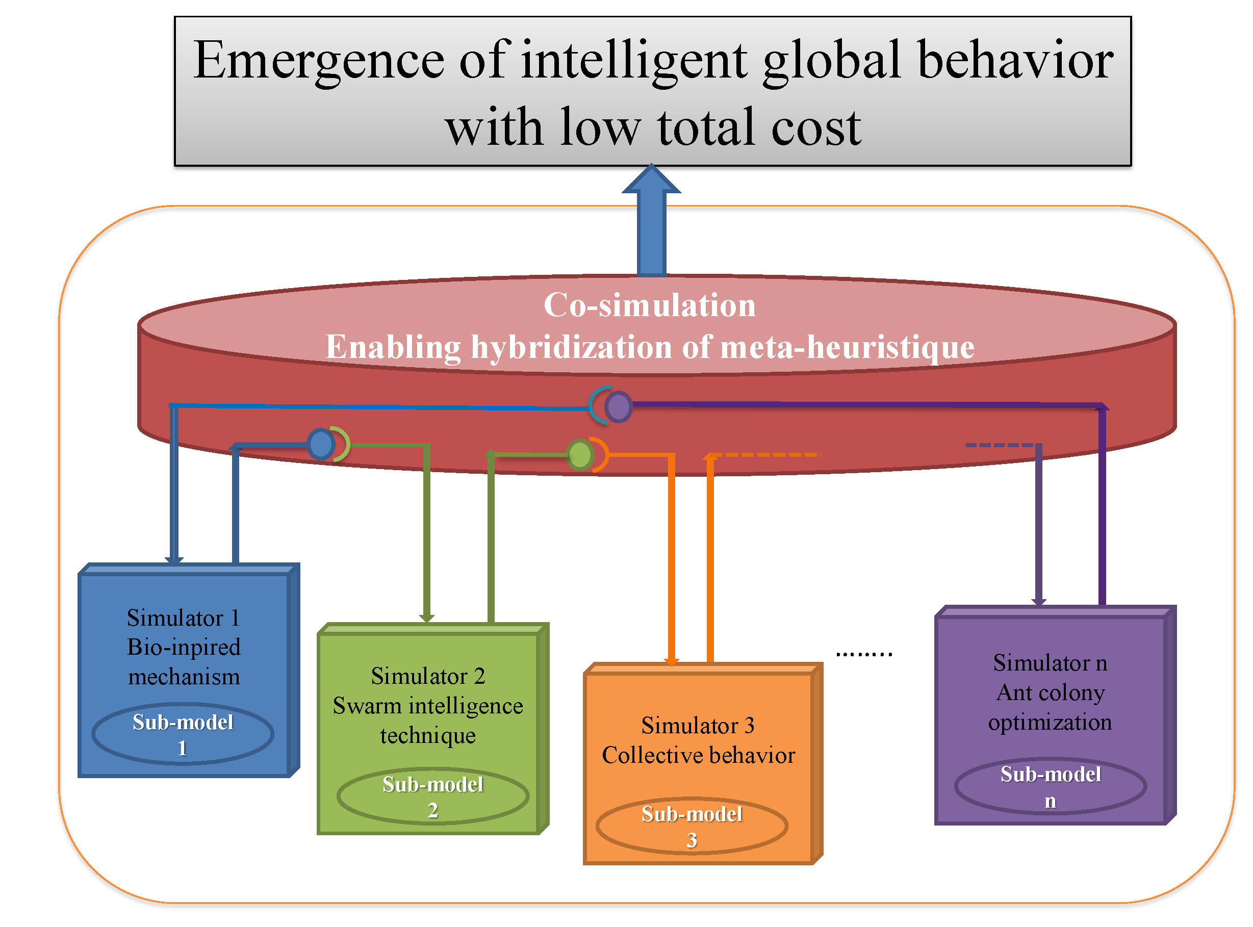
Co-simulation is applied in many different multidomain systems [
10]. It is proposed to address the issues and challenges of complex systems [
11]. In this context, decomposed components of a complex system are modeled by different sub-models, then simulated using a simulator for each sub-model. Co-simulation enables exchanging coupling connections to achieve the behavior of the whole complex system as shown in
Figure 1. The co-simulation middleware named Multi-agent Environment for Complex SYstem CO-simulation (MECSYCO) allows the integration of several modeling and simulation software to co-simulate the dynamic behavior of a complex system. MECSYCO makes the possibility to compare simulation results, swap, add, or remove models.
This paper aims to address the challenge of showing the impact of simulating a VRP multi-model as several interacting simulators by reducing the traveled distance and the obtained time during vehicles routing with the aim to satisfy clients demands. In this context, we will design and implement multiple VRP models as complex systems with several perspectives of multi agent simulators. Each simulator in the proposed solution solves different objectives of the VRP and then makes them interact into the co-simulation platform. Multi agent simulators that represent the VRP models are developed using Netlogo and the whole system is reproduced based on the MECSYCO co-simulator. We observed that the interacting VRP models provide high quality solutions by minimizing significantly the cost of services offered to the clients, in terms of computational time and travel distance.
The rest of this work is organized as follows: In
Section 2, we present the summary of the related multi-simulation of complex system research and introduce an overview of the used platform in the co-simulation and we describe the problem formulation of the VRP. The proposed solution is presented in
Section 3.
Section 4 provides the implementation details and the experiments results.
Section 5 concludes the work and give some future work avenues.
2. Related Work
To better simulate the behavior of the whole complex and dynamic system, multi-modeling and co-simulation are used to provide a strategy that collects a set of models from different discipline [
12]. The modular architecture in the multi-agent environment of complex system co-simulation middleware offers the integration of heterogeneous simulators and models. In the literature, several works such as [
5,
13], have been proposed for the simulation of the complex system as interacting models for reproducing the behavior of the entire system. The work of [
14] captures the improvement of decomposing and integrating continuous systems using MECSYCO as discrete environment. In [
15], the authors designed the co-simulation of complex system with integral multi-agent simulators, while MECSYCO was used in [
16] to integrate the modeling and the simulation tools to co-simulate the complete cyber-physical system.
The hybridization of meta-heuristics in the multi-agent system is used to facilitate the development of meta-heuristic frameworks’ optimization. In addition, the development of hybrid meta-heuristics is flexible in multi-agent systems and it offers simultaneous exploration of various areas of the research space [
17].
Several studies have been performed to solve different variations of VRP by using multi-agent systems [
18]. The work of [
19] uses the reinforcement learning and pattern matching to provide a multi-agent distributed framework where each agent adapts itself. In [
20], the authors solve the VRP with Time Windows (VRPTW) by exploiting the principle of reinforcement learning to improve the agent actions based on the solutions generated by other agents and the environment interactions.
To improve the result of VRP, this paper aims to create an interacting VRP model by combining the multi-agent simulators to reproduce the entire VRP multi-model. From the literature, we observe that there is no proposal in multi agent systems that integrates simulators into a co-simulation platform to reproduce the entire VRP multi-model.
2.1. Co-Simulation of a Complex System
MECSYCO has been used as a middle-ware to simulate and model complex systems which allows the utilization of existing simulators for the implementation of heterogeneous and numerical simulations. MECSYCO focuses on both, the DEVS common formalism proposed by [
21] that uses a discrete-event abstraction for the design of dynamic system [
22], and on the Agent and artifact architecture using a multi-agent concepts [
13] to perform the heterogeneous co-simulation of complex system. In this case, each model or simulator has been considered as an agent and the interaction between simulators corresponds to the indirect cooperation between agents using the defined concept of artifact in [
23]. Coupling artifact aims to determine the input output connections between two models and to create the model agent (m-agent) which uses the artifact for leading their model and interchanging input/output data. MECSYCO manipulates a model as various composed models in interactions without a global coordinator using a simulator for each model [
24]. This step occupies the management of decentralized multi model simulation in order to integrate several aspects of the same system into a coherent one and to deal with the main challenges of modeling and simulation of a complex system. On the other hand, MECSYCO already includes integrated simulators such as multi agent platform Netlogo, which is frequently used for simulating complex systems and modeling natural and social phenomena.
2.2. Mathematical Formulation of the Problem
This section deals with the mathematical formulation of the problem. In the combinatorial optimization field, VRP is one of the most challenging research problems. The issue was studied more than 40 years ago. It involves defining the best sequence of routes for a fleet of vehicles to provide the service to a specific set of clients. The fleet of vehicles is situated at a central depot, every vehicle has certain capacity and each client has a given demand. The aim is to optimize the total traveled distance to serve a geographically dispersed group of clients [
25]. First, we have the following data:
One depot;
A set of commands;
A fleet of vehicles.
The objective is to reduce the total traveled distance from a depot to serve clients, using a similar fleet of vehicles. The issue of solving the VRP faces several design challenges and focuses on the assignment of clients to the routes. This process involves the determination of several routes for each depot by (1) assigning each client to a unique route without exceeding the capacity of the vehicle, and (2) determining a series of clients on every vehicle route. Hence, the mathematical formulation of the vehicle routing problem can be described as follows:
R denotes the set of nodes, , with is the depot and is the client;
V denotes the sets of vehicles;
N is the number of all clients;
M is the number of vehicles;
is the capacity of vehicle k;
E is the edge set between nodes defined as: ;
is the demand of client i;
is the cost of transporting one unit from node i to node j;
is 1, if vehicle k travels from node i to node j; 0, otherwise,
is 1, if vehicle k offers service for client i; 0, otherwise.
From these definitions the objective function problem can be formulated as follows:
where Equation (
1) represents the objective function that aims to reduce the total travel cost and the constraints formulations are:
where Equation (
2) aims to ensure that every client is allocated in the single route and Equation (
3) is the capacity constraint set for vehicles. Whereas Equation (
4) is defined to assure that each client can be served only once and Equation (
5) ensures that all delivery vehicles must return to the original depot after finishing their task.
3. The Designed Model
The goal of this paper is to solve the VRP by building a complex simulation using a society of interacting co-evolving VRP models. The proposed approach provides a solution based on the agent and artifact concept [
23,
26,
27]. The simulation is performed by m-agents that manage their model and data exchange using artifacts.
The first task to do is to define a solution for solving each VRP model using an atomic VRP simulator. Then, the second task is to determine the input output connections between these simulators. The final task is to construct coupled interacting co-evolving VRP models.
3.1. Description of Atomic VRP Models
The routing and scheduling of a service correspond to the creation of vehicle routes for the depot. By assigning each client to a unique route and respecting the capacity of the vehicle the order of the clients on every vehicle route will be determined. To this end, we develop two models to solve VRP such that each model is to satisfy a different objective. The first is to try to minimize the total traveling distance and the second is to minimize the number of vehicles.
3.1.1. First VRP Model
We use ant colony optimization for the VRP, where the colony of ants is created from the depot. Each Ant constructs a route for vehicles that will serve the clients starting from the depot and returning to the same depot. The principle of the routing algorithm is described below, see Algorithm 1.
| Algorithm 1 Routing and sequencing of the first model |
- Require:
R, , ; - Ensure:
; - 1:
for () do - 2:
; - 3:
; - 4:
; - 5:
; - 6:
; - 7:
while do - 8:
for () do - 9:
; - 10:
end for - 11:
; - 12:
; - 13:
if then - 14:
; - 15:
; - 16:
; - 17:
; - 18:
else - 19:
- 20:
- 21:
; - 22:
end if - 23:
end while - 24:
end for - 25:
return;
|
The improvements of the solution shown in Algorithm 1 reached in successive iterations. In each iteration all ants in the colony travel between a pair of clients. The probability of an ant to visit an unvisited client is calculated based on the pheromone and the distance and a client will be chosen according to this probability. Then the ant checks if it can visit the given client, i.e., if its current load allows it to add the demand of the client and verify the vehicle’s capacity violation. If yes, the ant visits the specified client (adding client’s demand and indicating it as selected). Otherwise, the ant ends the current trip with empty load (returning to its colony) and the algorithm restarts a new trip. We apply the following equations for a client
i to choose the next client
j
where
is the probability of the point
i to choose point
j,
is the strength of pheromone trail between point
i and
j,
is the coefficient that controls the influence of the pheromone trail
,
is the coefficient that controls the influence of the visibility
, and
R is a set of clients.
At the end of each iteration, the pheromone trail evaporates according to the following equation:
where
is the coefficient of the pheromone evaporation and the update state is calculated by applying the next equation:
where
3.1.2. Second VRP Model
VRP of the second model uses a similar algorithm routing and sequencing of the first model. The difference is that each ant in this model tries to reduce the number of vehicles to visit all clients and to add all possible ones whose demand does not exceed the capacity of the current vehicle. The algorithm of the second model is formulated as follows, see Algorithm 2.
| Algorithm 2 Routing and sequencing of the second model |
- Require:
R, , ; - Ensure:
; - 1:
for () do - 2:
; - 3:
; - 4:
; - 5:
; - 6:
; - 7:
; - 8:
while do - 9:
while do - 10:
for () do - 11:
; - 12:
end for - 13:
; - 14:
; - 15:
; - 16:
if then - 17:
- 18:
- 19:
; - 20:
end if - 21:
end while - 22:
; - 23:
; - 24:
; - 25:
; - 26:
end while - 27:
end for - 28:
return;
|
In Algorithm 2, the ant checks if its current load allows it to add the demand of the chosen client and verifies the vehicle’s capacity violation. If yes, the ant visits the specified client (adding client’s demand and indicating it as selected). Otherwise, the ant selects another unvisited node according to the calculated probability. When all clients have been visited, the ant ends the current trip with empty load (returning to its colony) and the algorithm begins a new trip. We improve the solution by local search and we use a two-opt local search algorithm in the end of both Algorithms 1 and 2.
3.2. Structuring VRP Multi-Model
In order to co-simulate the multi-model of VRP, we use MECSYCO, which allows to lunch of several VRP models. In this approach, we focus on the reuse of atomic VRP models defined in
Section 3.1 and making them interact.
Figure 2 shows an overview on the model coupling of
and
.
As VRP models are created separately, each model has its own description and proceeds its own execution. It should couple these VRP models to reconstruct the entire multi-model using the co-simulation of MECSYCO. To this end, we define the connections between both models by specifying the input and output ports.
3.2.1. Exchanging Data between Simulators: Input and Output Connections
To predict the impact of co-simulation of VRP multi-model, we show the first model
which represents the solution of VRP using Algorithm 1, where the objective is to minimize the total traveled distance. The second model
implements Algorithm 2 that tries to minimize the total number of vehicles used to solve the same VRP. The aim in this case is to reproduce the VRP multi-model as a society of interacting and co-evolving models. We have to couple the two aforesaid models
and
using the concepts of Agent and Artifacts that are presented in
Section 1. To couple
and
we need to define the input and output ports of each model and the connections between them.
The solution is improved by successive iterations where every model, i.e.,
or
, shares the improved solution with the other.
and
read the input and try to improve their solution as illustrated in
Figure 3.
Specifically, when the model finds new best solution in a given iteration, it sends the following inputs to the model
: Set of edges belonging to the best solution (for each one of these edges the model sends a pair of nodes delimiting this edge).
P: Set of pheromones trail of each edge belonging to the best solution and the model retrieves these values of pheromone and modify its own values to have the new ones sent by .
These sent pheromones trail to the model will modify the pheromone trail of the same edges in for improving the best solution finding. According to the ant colony system, in Algorithms 1 and 2 the ant chooses the next node to be added to the solution according to
The cost of the best solution represented by the total traveled distance;
The edge with minimum distance to be traveled;
The edge with high value of pheromone trail.
The edge with high value of pheromone trail have a high probability to be added to the solution. Here, the model have edges with elevated values of pheromone trail from:
In the same way, when model
finds a new best solution, it sends its best solution to model
and replaces the current value of pheromone trail in this model by those of the new best solution in model
.
Figure 4 show more details on the behavior of models in interaction.
3.2.2. Interchanging Models
When executing two similar models of VRP, they give two different solutions in each iteration. Instead of coupling two different VRP models, we can simply integrate two similar models or two similar models . Here, we keep the same input and output connections as defined in the previous section. So, if one model has a good solution, it sends it to the second model and reciprocally. Specifically, when we couple two same models , they will have different solutions in each iteration, and the first one have better solution, send the following inputs to the second model :
: Set of edges belonging to the best solution.
P: Set of pheromones trail of each edge belonging to the best solution and the second model retrieves these values of pheromone and modify its own values to have the new ones sent by the first model .
This may impact on the solution of each model and redirect it to the best solution by reinforcing the pheromone of edges that have a good solution in each model. Moreover, we can study the evolution of the computational time when proceeding the co-simulation of VRP models, thereby the co-simulation of VRP models for finding a good solution.
Thus, we interchange models to compare different executions and study the accuracy of the best multi model.
Figure 5 shows the VRP models’ interaction graph.
By using MECSYCO we may launch more than one model of VRP at the same time following the routing algorithm defined in
Section 2. The execution gives two different solutions that are improved in each iteration. The whole architecture of the multi-model is modular, transparent and parallel so the simulation can be viewed as a set of distributed and reusable components such that:
The modeling is performed by model artifact.
Conducting the models is accomplished by the model-agents.
The coordination process is carried out by the coupling-artifacts.
As a result, we easily can add, remove or interchange models without being interested with coupling and coordination issues.
4. Implementation and Results
The VRP models are implemented using Netlogo [
28] which is an environment designed for modeling and simulating the natural and social experiences. We use MECSYCO to perform the co-simulation of the VRP models based on the following parameters of hardware:
Memory: 7.7 GB;
CPU: Intel® Core™ i5-8250U CPU @ 1.60GHz × 8;
Graphic Card: Intel® UHD Graphics 620 (Kabylake GT2);
Operating System: ubunto 16.04 LTS 64 bits;
Disk: 964 GB.
In the analysis, we study the behavior and the experiment results of VRP models on several VRP instances from [
29] and then we evaluate the improvement carried out by the co-simulation of the VRP multi-model in term of quality of obtained results and computational time.
4.1. Implementing VRP Models
In the definition and implementation of the VRP graphs using Netlogo, we use the turtles agent to represent nodes with their turtle variables. The coordinate of each client and the links agent are used to define the edge between two nodes. We use the link variables for determining for each edge the link cost of these two nodes and the value of pheromone trail.
Table 1 represents the result obtained by executing single model VRP: model
with BKS is the best-known solutions which were given by [
29], Perc-Dev is the percentage deviation of the result reached by the model
and Processing time (s) is the processing time for the execution of the model
.
Table 2 represents the result obtained by executing single model VRP, i.e., model
. Both models
and
are based on an ant colony system in their implementation, and they can interchange the following data: the cost of solution is calculated by the total traveled distance, edges belonging in the best solution found and the values of pheromone trail of these edges.
Other data can be exchanged between these models such as the route of the best solution or the route of each vehicle, etc. However, we skip these exchanged data to avoid more machine resources occupation because we must reserve more memory space to store the solution (routes) which takes a considerable time during the exchange.
4.2. Co-Simulation of VRP Multi-Model
In this section, we run different forms of combined models and perceive the improvement provided by their co-simulation. In order to develop interactive VRP multi-models, we use MECSYCO which offers multiple integrating VRP models by defining the input and output port of coupling artefact. VRP instances [
29] are a set of 100 instances created to offer a more universal and stable experimental setting.
Experiments were carried out in order to analyze the performance of the proposed VRP multi-model. The main objective is to assess whether the co-simulation has a direct impact on the qualitative performance of the obtained results. In this context, three composition are proposed for the interaction between the VRP multi-model used in the experiments:
Coupling two different VRP models: with .
Coupling two same VRP models: with .
Coupling two same VRP models: with .
Symbol A means: after co-simulation;
Symbol B means: before co-simulation;
Perc-Dev B is the percentage deviation of single model before co-simulation;
Perc-Dev A is the percentage deviation after co-simulation for two models in interaction;
Processing time B (s) is the processing time in second for just one model before co-simulation;
Processing time A (ms) is the processing time in milliseconds after co-simulation for two models in interaction.
Table 3 presents the co-simulation results of model
with
which demonstrate enhanced performance of the found solution in terms of percentage deviation and processing time compared with the execution of single model
.
Table 4 shows the result of the combination of the two same models
with
. We perceive that there is an improvement in the found solution compared with one model
in both the solution cost and the time of processing.
Table 5 shows the obtained results of integrating two different models
with
. We observe that there is an improvement in the found solution compared with the result of a single model
or
in terms of solution and time of processing.
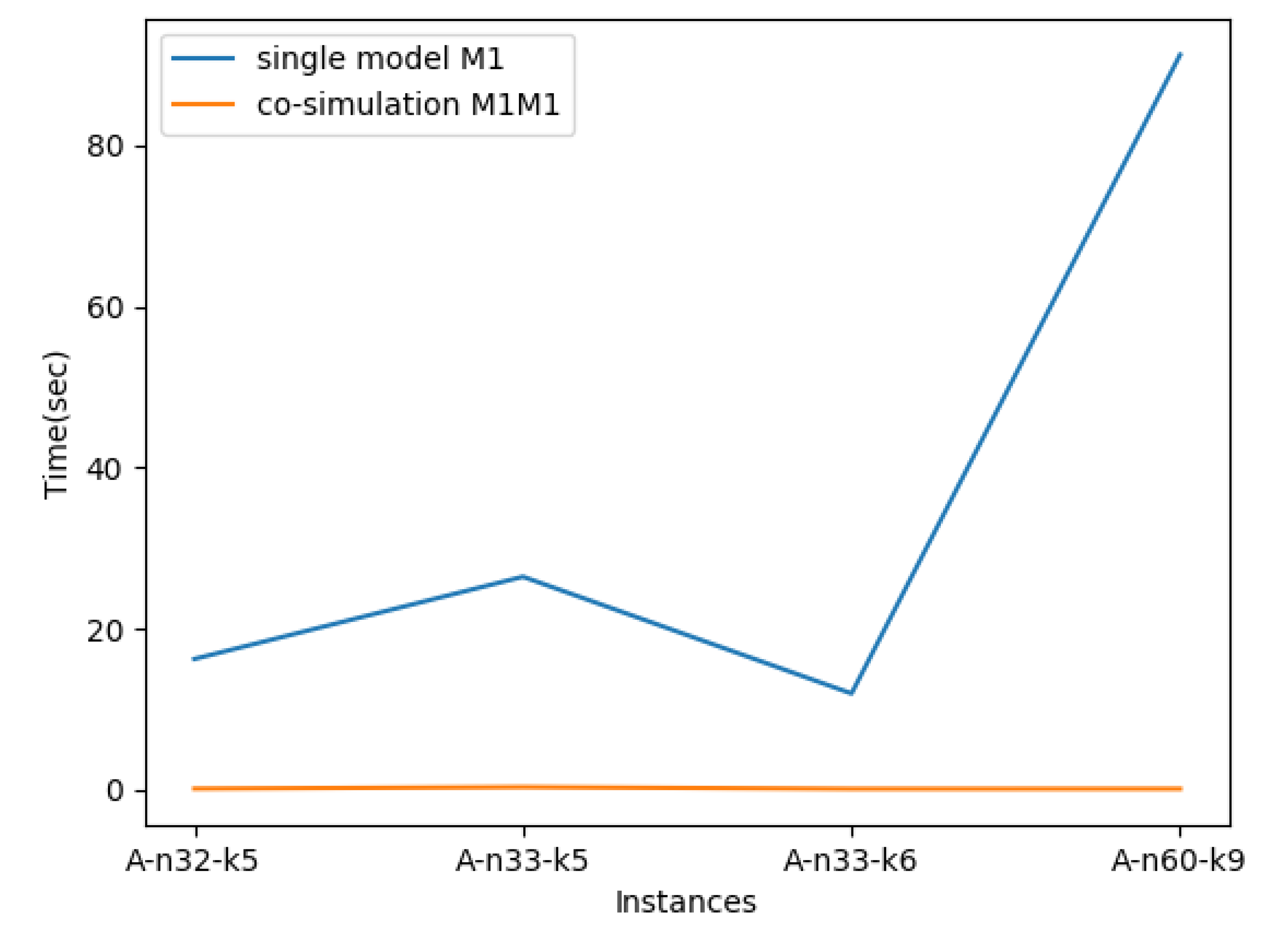
Figure 6 and
Figure 7 show the co-simulation processing time when coupling the same or different models. We conclude that the co-simulation of models is faster than the unique model
or
. On the other hand, during data exchange between models we proceed to post and read best solutions for each interacting model. Instead of sending the best solution as a sequence of routes, we choose to send it as separate edges with their pheromone trail. After the execution, we observe that this action has a significant impact on the behavior of the model in constructing its solution and the model builds better solutions quickly. In addition, it does not spend a lot of time interchanging data and occupies a reasonable memory size to store the best solution.
4.3. Discussion
We conducted several experiments in a single VRP model and multiple VRP models in interaction, Single VRP models implementing different algorithms of ACO metaheuristics gave close to optimal solutions; the VRP multi-model improved these results compared with single ones. We coupled
Always the result of coupled models was the best according to single model M1 or single model M2. It was especially time consuming.
Figure 8 displays the co-simulation processing time of the three coupled systems and shows that the coupled system using two same models
has the best result.
Co-simulation enables the integration of heterogeneous models/simulators homogeneously, in the future we can implement other types of metaheuristic and define the appropriate interchanging data between them, in order to study the amelioration of results in each different case.
5. Conclusions
This paper discusses the integration of VRP simulators created in Netlogo platform into MECSYCO co-simulation middleware. The proposed VRP multi-models in interaction implement ant colony meta-heuristic for solving two different objectives. The obtained results show the efficiency of better solution finding of VRP multi-models compared with single VRP models in terms of processing time and travel distance. We conclude that the type of data exchanged between models gives more qualitative performance to the solution short execution time to solve the problem.
In the future, we will evaluate the proposed approach by introducing other variants of VRP such as the Multi Depot Vehicle Routing Problem (MDVRP) and the Vehicle Routing Problem with Time Window (VRPTW). Moreover, the atomic VRP models can be implemented using other types of meta-heuristics and the combination of these models can be performed by defining other input and output connections.
Author Contributions
Conceptualization, S.S.G.; methodology, A.L.; software, M.H. and A.L.; validation, S.S.G. and A.L.; formal analysis, A.B.; investigation, A.E.; resources, M.A.; data curation, M.H.; writing—original draft preparation, S.S.G.; writing—review and editing, A.L. and M.H.; visualization, A.B. and A.E.; supervision, A.L.; project administration, A.L. and M.H.; funding acquisition, M.A. All authors have read and agreed to the published version of the manuscript.
Funding
This research received no external funding.
Institutional Review Board Statement
Not applicable.
Informed Consent Statement
Not applicable.
Data Availability Statement
Not applicable.
Acknowledgments
We would like to express our gratitude to Yagoub Mohammed Amine for their meaningful support of this work.
Conflicts of Interest
The authors declare no conflict of interest.
References
- Pokrovskii, V.N. Thermodynamics of Complex Systems; IOP Publishing: Bristol, UK, 2020; pp. 2053–2563. [Google Scholar] [CrossRef]
- Comin, C.H.; Peron, T.; Silva, F.N.; Amancio, D.R.; Rodrigues, F.A.; da F. Costa, L. Complex systems: Features, similarity and connectivity. Phys. Rep. 2020, 861, 1–41. [Google Scholar] [CrossRef] [Green Version]
- Dorigo, M.; Floreano, D.; Gambardella, L.M.; Mondada, F.; Nolfi, S.; Baaboura, T.; Birattari, M.; Bonani, M.; Brambilla, M.; Brutschy, A.; et al. Swarmanoid: A novel concept for the study of heterogeneous robotic swarms. IEEE Robot. Autom. Mag. 2013, 20, 60–71. [Google Scholar] [CrossRef] [Green Version]
- Liboni, G. Complex Systems Co-Simulation with the CoSim20 Framework: For Efficient and Accurate Distributed Co-Simulations. Ph.D. Thesis, Université Côte d’Azur, Nice, France, 2021. [Google Scholar]
- Camus, B.; Bourjot, C.; Chevrier, V. Considering a multi-level model as a society of interacting models: Application to a collective motion example. J. Artif. Soc. Soc. Simul. 2015, 18, 7. [Google Scholar] [CrossRef] [Green Version]
- Nazari, M.; Oroojlooy, A.; Snyder, L.; Takác, M. Reinforcement learning for solving the vehicle routing problem. Adv. Neural Inf. Process. Syst. 2018, 31, 9861–9871. [Google Scholar]
- Vidal, T.; Laporte, G.; Matl, P. A concise guide to existing and emerging vehicle routing problem variants. Eur. J. Oper. Res. 2020, 286, 401–416. [Google Scholar] [CrossRef] [Green Version]
- Wang, Z.; Sheu, J.B. Vehicle routing problem with drones. Transp. Res. Part B Methodol. 2019, 122, 350–364. [Google Scholar] [CrossRef]
- Li, Y.; Soleimani, H.; Zohal, M. An improved ant colony optimization algorithm for the multi-depot green vehicle routing problem with multiple objectives. J. Clean. Prod. 2019, 227, 1161–1172. [Google Scholar] [CrossRef]
- Chen, W.; Ran, S.; Wu, C.; Jacobson, B. Explicit parallel co-simulation approach: Analysis and improved coupling method based on H-infinity synthesis. Multibody Syst. Dyn. 2021, 52, 255–279. [Google Scholar] [CrossRef]
- Gomes, C.; Thule, C.; Broman, D.; Larsen, P.G.; Vangheluwe, H. Co-simulation: State of the art. arXiv 2017, arXiv:1702.00686. [Google Scholar]
- Pierce, K.; Gamble, C.; Golightly, D.; Palacin, R. Exploring Human Behaviour in Cyber-Physical Systems with Multi-modelling and Co-simulation. In Proceedings of the International Symposium on Formal Methods, Pasadena, CA, USA, 24–27 May 2019; pp. 237–253. [Google Scholar]
- Siebert, J.; Ciarletta, L.; Chevrier, V. Agents and artefacts for multiple models co-evolution. Building complex system simulation as a set of interacting models. In Proceedings of the Autonomous Agents and Multiagent Systems-AAMAS 2010, Toronto, ON, Canada, 10–14 May 2010; pp. 509–516. [Google Scholar]
- Paris, T.; Tan, A.; Chevrier, V.; Ciarletta, L. Study about decomposition and integration of continuous systems in discrete environment. In Proceedings of the 49th Annual Simulation Symposium (ANSS 2016): 2016 Spring Simulation Multi-Conference (SpringSim’16), Pasadena, CA, USA, 3–6 April 2016. [Google Scholar]
- Paris, T.; Ciarletta, L.; Chevrier, V. Designing co-simulation with multi-agent tools: A case study with NetLogo. In Multi-Agent Systems and Agreement Technologies; Springer: Berlin/Heidelberg, Germany, 2017; pp. 253–267. [Google Scholar]
- Camus, B.; Paris, T.; Vaubourg, J.; Presse, Y.; Bourjot, C.; Ciarletta, L.; Chevrier, V. Co-simulation of cyber-physical systems using a DEVS wrapping strategy in the MECSYCO middleware. Simulation 2018, 94, 1099–1127. [Google Scholar] [CrossRef] [Green Version]
- Silva, M.A.L.; de Souza, S.R.; Souza, M.J.F.; de Franca Filho, M.F. Hybrid metaheuristics and multi-agent systems for solving optimization problems: A review of frameworks and a comparative analysis. Appl. Soft Comput. 2018, 71, 433–459. [Google Scholar] [CrossRef]
- Mguis, F.; Zidi, K.; Ghedira, K.; Borne, P. Distributed approach for vehicle routing problem in disaster case. Ifac Proc. Vol. 2012, 45, 353–359. [Google Scholar] [CrossRef]
- Martin, S.; Ouelhadj, D.; Beullens, P.; Ozcan, E.; Juan, A.A.; Burke, E.K. A multi-agent based cooperative approach to scheduling and routing. Eur. J. Oper. Res. 2016, 254, 169–178. [Google Scholar] [CrossRef] [Green Version]
- Silva, M.A.L.; de Souza, S.R.; Souza, M.J.F.; Bazzan, A.L.C. A reinforcement learning-based multi-agent framework applied for solving routing and scheduling problems. Expert Syst. Appl. 2019, 131, 148–171. [Google Scholar] [CrossRef]
- Kim, T.G.; Praehofer, H.; Zeigler, B. Theory of Modeling and Simulation: Integrating Discrete Event and Continuous Complex. Dynamic Systems. 2000. Available online: https://www.semanticscholar.org/paper/Theory-of-Modeling-and-Simulation%3A-Integrating-and-Zeigler-Praehofer/92131a3aed0d72ccfe92364eee87e228c9c773e6 (accessed on 29 March 2022).
- Van Tendeloo, Y.; Vangheluwe, H. Discrete event system specification modeling and simulation. In Proceedings of the 2018 Winter Simulation Conference (WSC), Gothenburg, Sweden, 9–12 December 2018; pp. 162–176. [Google Scholar]
- Ricci, A.; Viroli, M.; Omicini, A. Give agents their artifacts: The A&A approach for engineering working environments in MAS. In Proceedings of the 6th international joint conference on Autonomous Agents and Multiagent Systems, Honolulu, HI, USA, 14–18 May 2007; pp. 1–3. [Google Scholar]
- Camus, B.; Vaubourg, J.; Presse, Y.; Elvinger, V.; Paris, T.; Tan, A.; Chevrier, V.; Ciarletta, L.; Bourjot, C. Multi-Agent Environment for Complex Systems Cosimulation (Mecsyco)-Architecture Documentation. 2016. Available online: http://mecsyco.com/dev/doc/User%20Guide.pdf (accessed on 29 March 2022).
- Savelsbergh, M. Vehicle Routing and Scheduling; Technical Report; Georgia Tech Supply Chain and Logistics Institute: Atlanta, GA, USA, 2002. [Google Scholar]
- Omicini, A.; Ricci, A.; Viroli, M. Artifacts in the A&A meta-model for multi-agent systems. Auton. Agents Multi-Agent Syst. 2008, 17, 432–456. [Google Scholar]
- Ricci, A.; Piunti, M.; Viroli, M. Environment programming in multi-agent systems: An artifact-based perspective. Auton. Agents Multi-Agent Syst. 2011, 23, 158–192. [Google Scholar] [CrossRef]
- Gooding, T. Netlogo. In Economics for a Fairer Society; Springer: Berlin/Heidelberg, Germany, 2019; pp. 37–43. [Google Scholar]
- Uchoa, E.; Pecin, D.; Pessoa, A.; Poggi, M.; Vidal, T.; Subramanian, A. New benchmark instances for the Capacitated Vehicle Routing Problem. Eur. J. Oper. Res. 2017, 257, 845–858. [Google Scholar] [CrossRef]
| Publisher’s Note: MDPI stays neutral with regard to jurisdictional claims in published maps and institutional affiliations. |
© 2022 by the authors. Licensee MDPI, Basel, Switzerland. This article is an open access article distributed under the terms and conditions of the Creative Commons Attribution (CC BY) license (https://creativecommons.org/licenses/by/4.0/).


 ,
, 


