Article

Models versus Datasets: Reducing Bias through Building a Comprehensive IDS Benchmark

1
Department of Computer Information Sciences, University of the Cumberlands, 6178 College Station Drive, Williamsburg, KY 40769, USA
2
Department of computing and cyber security, University of Texas A&M San Antonio, One University Way, San Antonio, TX 78224, USA
*
Author to whom correspondence should be addressed.
Future Internet 2021, 13(12), 318; https://doi.org/10.3390/fi13120318
Submission received: 10 November 2021 / Revised: 6 December 2021 / Accepted: 16 December 2021 / Published: 17 December 2021
(This article belongs to the Special Issue Machine Learning Integration with Cyber Security)

Abstract

:
Today, deep learning approaches are widely used to build Intrusion Detection Systems for securing IoT environments. However, the models’ hidden and complex nature raises various concerns, such as trusting the model output and understanding why the model made certain decisions. Researchers generally publish their proposed model’s settings and performance results based on a specific dataset and a classification model but do not report the proposed model’s output and findings. Similarly, many researchers suggest an IDS solution by focusing only on a single benchmark dataset and classifier. Such solutions are prone to generating inaccurate and biased results. This paper overcomes these limitations in previous work by analyzing various benchmark datasets and various individual and hybrid deep learning classifiers towards finding the best IDS solution for IoT that is efficient, lightweight, and comprehensive in detecting network anomalies. We also showed the model’s localized predictions and analyzed the top contributing features impacting the global performance of deep learning models. This paper aims to extract the aggregate knowledge from various datasets and classifiers and analyze the commonalities to avoid any possible bias in results and increase the trust and transparency of deep learning models. We believe this paper’s findings will help future researchers build a comprehensive IDS based on well-performing classifiers and utilize the aggregated knowledge and the minimum set of significantly contributing features.

Graphical Abstract

1. Introduction

Growing consumer, business, and industrial demand for advanced Internet of Things (IoT) solutions creates unique challenges to securing these devices. IoT devices are limited in resources such as memory, disk space, and processing power. Therefore, traditional security solutions (firewall, antivirus, software patches) applicable to personal computers do not adequately secure the growing number of IoT devices [1]. Unlike personal computers, these small devices not only lack built-in robust security features, but manufacturers also do not consistently deliver security patches and upgrades after selling the devices [2]. Naïve users either do not change the default passwords or set strong or difficult-to-remember passwords; this makes the devices vulnerable to various cyber-attacks. By using advanced mining tools, adversaries can easily takeover these devices remotely by finding many access points and penetrating deep into the network [3]. Once compromised, thousands or possibly millions of IoT devices can be controlled by a command and control (C&C) server to launch various large-scale attacks such as Distributed Denial of Service (DDoS) on critical national infrastructure and websites.
In order to secure IoT devices, a drastic change in security approaches and a paradigm shift are required [4]. A common and widely adopted network attack detection approach is known as anomaly-based (also known as behavior-based) Intrusion Detection System (IDS). This approach provides robust capabilities to detect various known and zero-day cyber-attacks by analyzing network traffic [5]. Researchers have been proposing anomaly-based IDS solutions for IoT environments using different Machine Learning (ML) and Deep Learning (DL) models trained on benchmark network datasets. Even though anomaly-based IDS provides good attack detection results, it may generate high false-positive detection results if not appropriately built [6]. An increase in false-positive results would undermine the system’s performance in detecting attacks. Unfortunately, many cyber-attacks and their variants are not so easy for an IDS to detect.
Several critical factors must be considered to create a proper and comprehensive security solution for IoTs to prevent large-scale attacks. The most important factors involve the quality and reliability of the benchmark datasets and their various features that contribute the most to providing a high attack detection rate. Regarding data quality and reliability, many recent IoT IDS research studies have been proposed based on very old benchmark datasets such as KDD CUP 99 [7,8], or NSL-KDD [9,10,11]. These datasets lack the modern day’s network traffic patterns and the various current attack information [5,12,13]. There are other important factors that most of the research studies lack in their proposed solution, such as (a) Many researchers report their DL model’s settings but nothing about explaining the model’s behavior on making specific predictions. (b) Researchers propose a DL-based IDS solution by reporting their findings on a single dataset, which produces biased results. Any model trained on a single benchmark dataset represents limited or restricted training; such models produce biased results when detecting different attack classes [14]. The goals of this research study are many-fold, including (a) to gather, extract, and analyze aggregate knowledge from various benchmark network datasets and look at the commonalities to avoid any possible bias in produced results; (b) mitigate dataset quality and reliability issues; (c) improve DL model transparency; (d) extract top features that influence the model predictions the most. Our results will provide insights and several benchmarks to future researchers when building a comprehensive IDS for IoTs. Some of the benchmarks would include finding which DL models perform well on which dataset; similarly, finding which DL models converge quickly and are suitable for a resource-constrained IoT environment. Our empirical results revealed that some of the DL models famous for processing sequential data such as LSTM, BLSTM, and BRNN are very expensive, take long hours to converge, and require millions of trainable parameters. However, it still does not produce better results compared to other models such as MLP, CNN, and TCN that converge in minutes, require minimum trainable parameters, and produce the best results. Although it is generally known that some models are computationally heavy than others, it is an important consideration point that computationally expensive models put additional burden on frequent model retraining on new data. Such IDS may not present an acceptable solution for IoT regardless of training them on the edge or fog layer. The more complex and deep the model is, the more computational and energy resources it needs, making model building and training burdensome and expensive. The results would help future researchers make a rational and knowledgeable decision on choosing a particular classifier for datasets with a large number of features.
The rest of the paper is organized as follows. Section 2 presents benchmark datasets used to explain various deep learning algorithms and the rationale for considering them for an IDS and libraries used to explain models and extract features that significantly contribute to making predictions. Section 3 presents our proposed framework in detail. Section 4 presents the experiments carried out using various datasets and classifiers. In Section 5, we compare the results of our proposed framework with the previous researcher’s work in the IDS field. Finally, the conclusion and future work is presented in Section 6.

2. Literature Review

IoTs are resource constraint devices built for a specific purpose. Due to limited resources and their ability to communicate over the internet and work independently, they are exposed to many cyber-attacks. Resource limitations prevent security experts from applying conventional security solutions such as firewalls, antivirus, and patches [1]. In contrast, access to the internet allows cyber-attackers to use sophisticated software to quickly overtake these devices and use them as bots to launch further large-scale distributed attacks on critical infrastructure and websites [15]. There are many attack types that can impact IoT systems. Some of them include distributed denial of service (DDoS), botnet, keylogging, phishing, spamming, click fraud, identity theft, and malware proliferation. However, the most common and the most dangerous are Denial of Service (DDoS) and botnet. Some of these attacks are active attacks because they occur during real-time network communication. They either affect the normal operations or alter the system resources, e.g., data alteration or flooding the target system (DDoS, DOS) to make it unresponsive to prevent it from serving any new requests. Contrary to active attacks, passive attacks monitor and analyze the traffic pattern by eavesdropping to find vulnerabilities such as open ports, low cipher usage, and unencrypted traffic [16]. Protecting the IoT environment is critical. Many research studies have been based on finding the optimal machine learning solution. However, most of them do not provide a comprehensive solution by investigating network traffic from various sources or building robust models that converge quickly and provide the best results. Some researchers trained their models on a single and old dataset (e.g., NSL-KDD), which lacks modern-day attacks [17]. An IDS must detect a large number of attack types because some of the DDoS attacks such as “Slowloris” slowly deplete server resources and are hard to detect [18]. In contrast, others such as “Jamming” attacks can quickly drain resources and have serious consequences [19].

2.1. Related Work

The performance of conventional ML approaches plateau and remains stagnant once a certain computational threshold has reached; in contrast, DL performance grows rapidly as the dataset size grows [10]. Therefore, our focus in this study is only on deep learning-based models. Due to the continuous changes in network attacks every year, it is important to train models on diverse datasets consisting of different attacks and also provide the ability to quickly retrain models on new traffic patterns to evaluate IDS performance [20]. The security experts need to be able to interpret the model’s output consistently and understand the factors and features that cause the model to make certain predictions [21]. Features have a significant impact on ML model predictions and their quality [22]. Many research studies have recently been performed on explaining model outputs [23,24,25,26]. The two common approaches to explain model output are post hoc, also known as model-agnostic and model-specific approaches. The model-agnostic approach has received much attention in the research community [27]. Model-agnostic approaches to explain machine learning models provide many advantages over model-specific interpretation approaches. One of the important ones is to allow researchers to build any machine learning model they desire without worrying about the model’s complexity and interpretability [28]. For a model-specific interpretation, it is difficult to switch to a new or existing model with a slight change in the model settings.
Many researchers have proposed deep learning-based IDS for IoT environments; however, few have explained their model’s output. For example, in [23], the authors tried to explain their model’s output, but their solution is not comprehensive. They only looked at a single dataset NSL-KDD to train the model and predict attacks. In another study, the authors only investigated the robustness of interpretable models [29]. Some researchers used Convolutional Neural Networks (CNN) to detect diseases using localized model interpretation only [30]. In another research, the authors used the NSL-KDD dataset to train a deep neural network and applied LIME and SHAP to explain the model behavior [31]. However, their solution only focuses on explaining a single classifier and using a single dataset, “NSL-KDD,” which is old and lacks recent attacks [32]; they have not used their research to find optimal classifier settings across various datasets. In [33], the authors used a localized explanation to interpret the model using an old dataset and Multilayer Perceptron (MLP).
This paper is a step forward from our previously published paper [34] which proves the bias issues in models that are trained on a single dataset. In our previous work, first, we replicated various DL-based models from many researchers using the same dataset, classifier settings, and the preprocessing steps; second, we proved the bias issue by switching the dataset to a new benchmark dataset that caused the good performing classifier to drop their performance considerably. In this paper, we overcome this limitation. Instead of building a model on a single dataset and a single DL algorithm, we incorporated multiple datasets and multiple algorithms to diversify the input data and the processing algorithm for optimal performance.

2.2. Benchmark Datasets

The dataset has a critical role in building and testing a holistic IDS solution. Deep learning models need a large volume of data for better classification and improved performance. Some of our goals in this study, as stated earlier, are (a) to gather, extract, and analyze aggregate knowledge from various benchmark network datasets and look at the commonalities to avoid any possible bias in produced results and (b) mitigate dataset quality and reliability issues. To achieve these goals, we gathered various benchmark network datasets to capture a diverse set of attacks, devices used for data collection, different traffic capture duration, and actual and simulated traffic patterns. Some of these datasets, such as KDD CUP 99 and NSL-KDD, are very old and not IoT specific; however, researchers have still used them extensively to build their models. Others similar to BoT_IoT are recent and provide IoT-specific traffic. Table 1 provides details of the datasets used in our empirical analysis.

2.3. Dataset Quality and Reliability Issues

Data quality is important and greatly affects the reliability and robustness of an IDS. Data quality problems impact model predictions and impact security experts’ decisions that rely on IDS results. From an IDS perspective, it is important to not only train ML-based models on clean and reliable data, but it is also important to diversify the data to cover a vast range of traffic patterns and minimize the model’s biased output towards limited traffic patterns. In ML, some of the common data quality issues consist of noisy or insufficient labeled data, imbalanced data, duplicate data, incomplete data, and inconsistent data. A dataset consisting of a few attack patterns cannot fulfill the IDS purpose. In the preprocessing steps of ML-based modeling, data quality issues are fixed using statistical or manual techniques to ensure models are trained with clean and reliable data only.
In [48], the authors emphasized the impact of poor-quality data on ML-based models’ performance. The authors argued that very few research studies pay attention to data requirements and quality issues. The authors presented eight data quality issues relevant to ML-based IDS. These include reputation, relevance, comprehensiveness, timeliness, variety, accuracy, consistency, and de-duplication. In [49], the authors empirically analyzed data quality issues and stated that the data quality issues in ML-based models cause compounding negative events, create downstream effects, and become a technical burden to manage over time.
Today, many ML-based IDS solutions are proposed by training the model on a single dataset. These models are proposed to assume that the training labels are accurately identified. However, this assumption is not fully accurate because the labels are manually created by a security expert who may lack the appropriate judgment; similarly, imbalanced class labels can impact the performance and accuracy of an ML model [50]. There are different approaches adopted by the researchers to mitigate dataset quality and reliability issues, such as removing noise in the labels, increasing unique input data instances to statistically represent the population, utilizing techniques such as bootstrapping or SMOT (Synthetic Minority Over-sampling Technique) [5] to overcome class imbalance issues. In this paper, we improved the data quality issues that may cause biased results by performing various preprocessing steps to clean the noise from the data and trained various models on multiple datasets containing unique attack classes and traffic patterns.

2.4. Deep Learning Classifiers for Sequential Data

Researchers have been proposing a vast range of ML and DL solutions for network anomaly detection. This paper focused our experiments on only those DL classifiers that are famous, commonly used, and are known to perform well on sequential data. Section 3 presents our proposed framework with various DL classifiers used in this study. Firstly, we implemented a Multilayer Perceptron (MLP), which is a feed-forward Neural Network and consists of an input, hidden, and an output layer. It has frequently been used for network anomaly detection [11,51,52,53,54]. Autoencoders (A.E.) are robust unsupervised neural networks. A.E. helps avoid data imbalance and dimensionality reduction and reconstruct errors while detecting anomalies [55]. Researchers have shown great interest in A.E. when solving anomaly detection, fault diagnostics, dimensionality reduction, compression, and other related problems.
A Recurrent Neural Network (RNN) is a powerful and famous algorithm to find hidden patterns in sequential data [56]. RNN captures temporal dependencies in the data by storing the data received earlier [57]. RNN’s are good at processing sequential data; however, they suffer from gradient vanishing problems, are challenging to train [58], and cannot remember longer sequences [59]. Long Short-term Memory (LSTM) is a specialized RNN that can remember information for a longer period using a memory cell. It overcomes RNN’s vanishing gradient problem [60]. LSTM’s consist of three gates, i.e., input gate, forget gate, and output gate [57]. The gates control access and information flow in the memory cell and prevent stored information from being overwritten with irrelevant information. Bi-directional LSTM (BLSTM) came to solve some of the problems in traditional LSTM, such as that LSTM cannot operate in both positive and negative directions [61]. Similarly, LSTM does not work for tasks requiring explicit and external memory [60]. BLSTM are good in processing sequential data in both time directions using forward and backward LSTM layers [62].
A Convolutional Neural Network (CNN) is primarily used for image classification and produces high accuracy when performing complex tasks [56]. A basic CNN consists of one or more convolutional, pooling, and fully connected layers. The 1D-CNN has been used in many IDS studies and produces good results in processing sequential data [63]. CNN’s main advantage over a feed-forward neural network is that each neuron in CNN only connects to a subset of input; this reduces the total number of network parameters and improves training time and process [64]. Temporal Convolutional Network (TCN) is a feed-forward network and is a variant of CNN that uses causal convolutions. A CNN architecture combined with causal padding makes it a causal convolution [65]. TCN is known to maintain a temporal sequence of data, which helps in preventing information loss. TCN allows better GPU optimization during training [66].

2.5. Feature Importance

Over the past many years, extensive research has been performed on building an optimal IDS for an IoT environment. However, researchers have been challenged to optimally handle the changing network traffic patterns, technology shifts, and large data volume management [67]. An essential operation in machine learning (ML) is finding the best features before training the models. Unfortunately, there are no commonly agreed-upon approaches on feature selection that can be applied to every problem on hand. Researchers sometimes use their judgment, experience, or statistical techniques such as Principal Component Analysis (PCA) to find the least number of optimal features. Each of these approaches aims to effectively handle large data sets with a large number of features without compromising model performance and accuracy. Once the representational features are extracted, they are used to train the ML classifiers and are applied to test the anonymous traffic patterns [68].
Selecting the important features is commonly performed manually in traditional ML approaches. The process is challenging, labor-intensive, time-consuming, and is prone to errors [57]. The feature selection computation time increases when the input dataset has a large number of features [69]. On the other hand, deep learning algorithms perform well on large datasets without explicitly performing feature selection [70]. However, some researchers still find benefits in performing feature selection in deep learning-based models [56]. For example, in one study, the authors used the NSGA-ii-aJG feature selection method with the CNN + LSTM model and achieved 99.03% accuracy [71]. On the other hand, in another study, the authors used DL’s capabilities to auto-select features to detect anomalies; their proposed LSTM model achieved a 99.98% precision score compared to the SVM model, which could only achieve an 88.18% precision score [57].
Deep learning models are inherently complex with a large number of hidden parameters, complex settings, multiple layers, and hidden nodes. Because of the complex nature of DL models, many researchers only report model settings and performance results but nothing about the output and findings of the model itself. Some researchers try to justify their classifier performance using techniques such as cross-validation, but DL models could still fail to learn important hidden representations that an expert human in the field might consider necessary. Similarly, a model may consider certain features important, which an expert human may not consider necessary.
Explaining model output is essential for various reasons, including (a) human curiosity about specific predictions [72], (b) making the model explainable to naïve humans, (c) enhancing and redesigning the model by analyzing its output to gain optimal performance, (d) understanding why specific wrong predictions were made, and (e) improving trust and confidence in the model’s decisions. Once a model is analyzed as a whole, or when individual predictions are deeply analyzed, it is assumed that models can be redesigned with a limited set of features for better results and performance. When a model is explained locally, its scope is limited to single-input data instance only. Individual probabilistic scores are calculated to express the predictions for an individual instance compared to all predictions. On the other hand, models can be explained as a whole with a global scope. The approach to explaining models can be built within a DL model itself or can be applied as a post hoc approach. However, model explanation within a model has a restrictive scope and can lead to significant changes with a slight change in model settings. On the other hand, researchers have shown interest in the post hoc approach that uses ad hoc methods and techniques to explain any model already built [73]. It is not easy to interpret complex deep learning models such as ensemble or hybrid models. For complex models, the post hoc approach provides a simpler approach to interpret model outputs. The following sub-section presents two state-of-the-art libraries commonly used in post hoc methods to explain models locally and globally.

2.5.1. Local Interpretable Model-Agnostic Explanation (LIME)

The LIME explains the individual predictions of any model by approximating it locally [74]. The output of LIME provides a quantitative and visual understanding of an instance and the model predictions in order for a naïve or expert person to build trust in a model and make effective decisions. LIME provides local fidelity of predictions, which may provide different results than global explanatory methods; in other words, features that LIME considers important for a local prediction might not be considered important by the global explainers and vice versa. LIME has some advantages over global model explainers such as SHAP; for example, it is computationally fast and converges quickly. Explaining an individual model prediction is faster compared to finding and aggregating global permutations. LIME uses an intuitive approach to analyze model output by providing variations in the input data. The variation in input data is generated by creating new perturb data from the original input. The new data are then used to train the model and interpret its predictions. An important pre-consideration must be made to specify the number of features we want to interpret the model when interpreting models. The higher the features, the better the trustworthiness of the model. Equation (1) represents a local interpretation of input data sample x:
i n t e r   p r e t a t i o n ( x ) = a r g m i n g G L ( f , g ,   π x ) + ( g )
where g represents an individual model from the list of available explainable models G (e.g., decision tree, linear regression) for the sample instance, x and f represent the original model (e.g., MLP) being explained. π x defines the proximity measure or weight between the original and sample data. L (f,g, π x) represents the fidelity function that will try to reduce the loss L (e.g., categorical cross-entropy) and measures the difference between the predictions made by the original model f and its representation g. Finally, Ω ( g ) represents the complexity of model g. LIME explains the model by trying to minimize the fidelity function and the complexity so naive humans can easily interpret the model.

2.5.2. SHapley Additive Explanation (SHAP)

SHAP is another popular method used to interpret model predictions for increased model transparency. It is based on coalitional game theory, which fairly distributes the payout among the features. SHAP measures each feature’s contribution towards the model output [75]. The two great advantages of SHAP include: (a) global interpretability, which provides a good explanation of each feature’s contribution (either positive or negative) to the model predictions across all permutations. (b) Local interpretability, which provides transparency through the local interpretability of each observation. Each observation x is assigned a corresponding SHAP value that can be applied to any model. SHAP computes the contribution of each feature to the predictions as follows:
g ( z ) = ϕ 0 + j = 1 M ϕ j z j
where g represents the explainable model of deep learning model f. z′ ϵ {0,1}M represents simplified features, also known as a coalition vector, where 0 means the feature value in the new data is not available in the original data, and 1 means the feature value in the new data is available in the original data. M represents the maximum coalition size, and ϕ j ϵ R represents the feature attribution, quality, or impact of feature j on predictions. A large value of ϕ j presents a strong positive impact of a feature on predictions.
Depending on the model type, SHAP provides various explainers [76]; some of the commonly used explainers are as follows: (a) TreeExplainer can be used to explain tree-based classifiers such as XGBoost, random forest, etc. (b) KernelExplainer can be used to explain any function, (c) DeepExplainer only explains deep neural networks, and (d) GradientExplainer can also be used to explain neural networks frameworks, such as TensorFlow, Keras, and Pytorch [77].

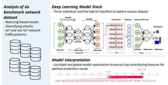
3. Proposed Framework

Many research studies have been performed on anomaly detection where researchers report their model settings and performance measures. Our proposed methodology overcomes some of the important limitations in previous research studies, where researchers do not report their proposed model’s output itself but what features contributed to the model to make certain predictions or influence the overall model performance. Similarly, many previous research studies generate bias results due to training the models only on a single dataset consisting of a limited network traffic pattern. A single dataset does not classify a vast range of attack classes and may lack recent traffic patterns [11]. This paper explores the output of various DL models by implementing SHAP and LIME, analyzing predictions, finding commonalities to avoid bias, improving classifier quality and reliability, and extracting top contributing features that influenced the model predictions most. Figure 1 depicts the proposed framework overview.
To avoid the bias issue of a single dataset, we used various benchmark datasets. The details of these datasets are presented in Section 2.1. Datasets are then trained on eight different deep learning models known for processing sequential data and producing good results in anomaly detection. In our approach, we first implemented single classifiers and then hybrid classifiers to find the impact on classification. Detailed summary results were captured with numerous valuable information such as model settings, trainable parameters, training time, and model size, etc. The novelty of this work is reducing bias results and improving model interpretability by using LIME to explain local predictions and SHAP to explain both local and global model output. The top 20 important contributing features were extracted, which were then used to enhance the DL models by improving model settings, performance and choosing the best classifier for a resource constraint environment.
Our experiments involve various datasets and DL models. To preserve the space, we only present the architecture of one of our hybrid models, “Autoencoder + TCN,” in Figure 2. The same architecture has been used for other hybrid model implementations shown in Figure 1. In other implementations, we replaced the “TCN Structure” block in Figure 2 with LSTM, BRNN, or BLSTM. Model-specific settings are reported in Table 2 (individual classifiers) and Table 3 (hybrid classifiers). In this architecture, first, the autoencoder takes the input shape of the dataset, reduces its dimensions to a smaller size (also known as latent space) and then reconstructs the original data from the compressed representation. Autoencoders generate reconstruction errors and guarantee very high accuracy with low latency detection [78]. The output of autoencoders is passed into a TCN structure. The pooled outputs of TCN block layers are flattened into a one-dimensional array and are passed to a fully connected layer. The last layer is passed with total output classes using the “softmax” activation function to make predictions on each label.
The TCN block in Figure 2 is the layered implementation of the dilated causal convolution of the TCN architecture. Figure 3 reflects the details of this model. TCN block takes three parameters as follows:
T C N   b l o c k   ( f i l t e r s ,   k e r n e l _ s i z e ,   d i a l a t i o n _ r a t e )
where “filters” are similar to units in LSTM, and they affect the model size. A larger filter size is preferred. It helps to train the model in parallel and faster, unlike RNN and LSTM, where predictions must wait for the predecessor results [79]. In TCN, a longer input sequence can be processed as a whole instead of sequentially. The “kernel_size” parameter determines the size of each filter in each convolution layer. It helps to calculate how much of the input is used to calculate each value in the output. A larger kernel_size helps detect complex features. The “dialation_rate” parameter represents a fixed step between two adjacent filters. A “dilation_size=1” is the same as a regular convolution in a CNN network. A larger dilation rate captures a bigger input range on the top convolution layer, making a TCN more receptive [79]. Our TCN structure starts with a CONV1D dilated causal convolution layer, followed by a batch normalization layer to obtain high accuracy values and increase model training. We then implemented a Rectified Linear Unit “Relu” to allow quick network convergence. We then added a “Dropout” layer to avoid over-fitting and added regularization by randomly dropping 30% of weights connected to certain nodes during the training process. The same layer structure was repeated in the TCN block and is shown in Figure 3.

4. Experiments, Results, and Analysis

This section discusses the experimental setup and various findings. We present our rigorous experiments in various parts. First, Table 2 shows the summary of individual classifiers, and Table 3 shows the hybrid classifier’s implementation summary. All experiments presented in Table 2 were executed with 20 epochs and a batch size of 256. Several pieces of valuable information were gathered, including (a) trainable parameters, (b) training time, (c) model size, (d) accuracy, (e) epochs, and batch size. Two separate experiments were performed on NSL-KDD and UNSW_NB15 datasets; In (*a), models were trained and predicted on the given training and testing set. In (*b), we merged the training and testing set, shuffled the dataset, and recreated a new training and testing set based on the 70:30 split ratio. In (*c), models were trained on the given full dataset and created a training and testing set based on a 70:30 ratio. Second, Figure 6 shows the SHAP’s local explanation of the KDD CUP 99 dataset. To conserve space, we only presented a single prediction from a single dataset. Figure 7 also shows the local explanation of one of the predictions using LIME. Lastly, Figure 8 shows the results of SHAP’s global explanation by listing the top 20 most important contributing features.
Table 2 shows that the LSTM model requires over 3 million trainable parameters, thus requiring a longer training time than MLP and CNN. Running the model on UNSW_NB15 (*c) requires over 8.5 h, making it an expensive algorithm for a resource-constrained IoT environment. Figure 4 compares the accuracy comparison of each of the classifiers. All three algorithms return similar accuracy, with LSTM performing slightly better on the UNSW_NB15 (*a) dataset.
Table 3 shows the summary of hybrid classifiers. The “Autoencoder + TCN” takes on average the least number of trainable parameters around 199K, whereas “Autoencoder + BLSTM” takes the most over 9.2 million parameters. All other classifiers also require a large number of parameters, with “Autoencoder + LSTM” taking over 3.3 million and “CNN + LSTM” taking over 3.2 million trainable parameters. For an IoT environment, “Autoencoder + TCN” is convenient due to a smaller than 3 B, shorter training time, and better accuracy than other models.
Figure 5 shows the accuracy comparison of each of the hybrid classifiers. “Autoencoder + TCN” returns better accuracy compared to other algorithms. “Autoencoder + BRNN” returns very low accuracy with only 23.30% on N-BotIoT and 31.90% on UNSW_NB15 (a*) datasets. Model training time is also an important concern in a live environment. As shown in Table 3, algorithms such as “CNN + LSTM” took over 9 h to converge on UNSW_NB15 (*c) dataset. Models that converge faster can be trained multiple times during the day with new attack information to keep them up-to-date.

4.1. Individual Prediction Interpretation—Localized Explanation

We performed two analyses to look for a suitable measure of feature importance. SHAP and LIME provide a localized explanation of a specific prediction. Both local and global explanations show the complexity of models when making predictions. SHAP local explanation in Figure 6 visually shows the features considered important by the classifier in making an individual prediction. The prediction reflects the probability that the input traffic is a DOS attack. Results showed that the base value of 79.24% (model’s average prediction over the training set) would be predicted if the features to the current output f(x) were unknown. However, the classifier was able to predict the DOS attack with 100% accuracy. The top features that predict the attack are shown in red color and are count, dst_host_count, service_ecr_i, service_http, etc., whereas the blue features dst_host_srv_count drives the prediction value lower. The larger arrow size of the count shows the magnitude of this feature’s effect on making a classification decision.
Figure 7 shows the local explanation of a DoS vs. NOT DoS attack using LIME. The classifier predicts that the traffic is a DoS attack, and the LIME bar chart highlights the importance given to the most relevant features that led to the prediction. As shown in Figure 7, protocol_type_udp, logged_in, count, srv_count, and dst_host_srv_count are depicted as contributing to the “DOS” prediction, while serror_rate is against it. Cybersecurity experts can review these granular details to make an informed decision about trusting the model’s predictions.

4.2. Model Interpretation—Global Explanation

Similar to the local explanations presented in Section 4.1, global explanations also interpret the model by providing insights on input features, patterns, and the output correlation to promote model behavior transparency [73]. SHAP provides various methods to explain models. This paper’s scope is limited to deep learning models only, so we used DeepExplainer and GradientExplainer to extract important contributing features in the overall model output. Analyzing global explanations of models is important to understand general model behavior when dealing with large datasets and a large number of features. We implemented multiclass classification in our experiments and extracted the top 20 contributing features for each attack type. The experiments were run on all eight datasets and eight DL classifiers. To conserve space in the paper, we present the visual output of only two datasets in Figure 8. Figure 8a shows the top 20 most contributing features extracted from the BoT_IoT dataset, and Figure 8b shows the top 20 most contributing features extracted from the UNSW_NB15 dataset. Different target classes are shown in color legends as well.
SHAP adds the absolute Shapley values per feature per target label to identify important features globally and sorts them with maximum values on the top and minimum values at the bottom. The visual graph in Figure 8 depicts important contributing features from top to bottom in different colors. The process is represented in Equation (3).
I j = i = 1 n | ϕ j ( i ) |
where ϕ j ( i ) refers to the Shapely value for feature j in the i-th data; N is the total number of samples in the dataset; and I_j is the average Shapley value of the feature j. Briefly, Figure 8a depicts dur as the most important feature followed by sum, N_IN_Conn_P_DstIP, etc., in the BoT_IoT dataset. Similarly, Figure 8b depicts sttl as the most important feature, followed by ct_state_ttl, dttl, smeansz, etc. Further details and analysis of which features each classifier considered important are presented in Section 4.3. Global explanation helps to refine further models towards building an online IDS, which can look at only a limited set of network traffic features to make decisions quickly in an unsupervised manner.

4.3. Top Contributing Features

This section presents the aggregated knowledge of important features identified by each of the eight DL classifiers from all eight datasets. Our approach was to extract the top 20 features and is divided into three sub-categories, (a) Table 4 provides a list of features identified by every classifier. These features must be considered the most important features (b) Table 5 provides a list of features identified by six or more classifiers, and (c) Table 6 provides a list of features identified by five or fewer classifiers. Each classifier reports features sorted by top contributing to low contributing; however, we are not reporting the ordering sequence here because it will require a very big table size if we report the individual output of eight classifiers on eight datasets. Our goal is to present an aggregated knowledge and report those features to which all or the majority of classifiers have been given some importance in the top 20 list regardless of the ordering sequence.
Table 4 reveals that some features in each of the datasets carry more importance than others. Every classifier picked such features in making decisions. Similarly, as shown in Table 5, some other features were given a little less importance by only one out of eight classifiers who did not think it was an important feature. Lastly, many other features were considered important by five or fewer classifiers. These features in the third category still carry importance but not as much compared to the first two categories.
Feature selection has an important role in machine learning. For an IDS, eliminating unnecessary features can help in improving the performance, reducing the computational cost, and early detection of malicious traffic. In addition to these benefits, feature optimization also helps to find a subset of features that can produce better classification results. This paper, based on the output of multiple deep learning algorithms and datasets, presented a minimum set of top contributing features consisting of diverse attack classes and algorithms. From the top contributing features shown in Table 4, Table 5 and Table 6, multiple traffic flow-based features are discovered by each algorithm, for example, source and destination IP addresses, ports, protocol, and flags used. Network flow-based features provide metadata details of many securities-related details of network activities. From the traffic flow information, security experts can identify a given session’s full TCP/IP information to analyze a particular activity better. Network flow-based features also present a good use case to detect large-scale attacks such as DDoS and DoS. These attacks generate excessive network traffic, and detecting them using individual packets could consume all available resources; therefore, it is optimal to analyze flow-based features to detect large-scale attacks [80].
The experimental results and identifying the top contributing features in each dataset by a specific model are a step towards future research where authors plan to further optimize each of the models by training them using only top contributing features shown in Table 4, Table 5 and Table 6. Some DL models generate thousands of neurons and trainable parameters, as shown in Table 2 and Table 3. For a large dataset with many features, this leads to the problem of “Curse of Dimensionality.” Reducing the number of input features helps solve this problem [81]. In [71], the researchers reported accuracy improvement with a 5-fold reduction in training time by selecting reduced features for model training compared to total feature space.

5. Models versus Datasets, a Comparison Study

The performance of an ML-based model depends on multiple factors. For example, the dataset’s size directly impacts the model training time. Although DL is known to provide optimal performance on large datasets, the bigger the training dataset, the longer it takes to train the model. Therefore, researchers have started exploring options to train DL-based models with distributed training using TPU’s and GPU’s that provide better computational capabilities [82]. Another important impact on DL-based models is the datasets with a large number of features. As shown in Table 2 and Table 3, the LSTM model generates over 3 million trainable parameters in individual classifiers, whereas “autoencoder + BLSTM” generates over 9 million trainable parameters on multiple datasets. Models that generate a large number of trainable parameters require longer training time and have bigger model sizes. Domain shift is another issue that impacts DL performance [83]. A general assumption in DL-based modeling is that the training and testing data come from the same distribution under the same settings. This assumption contradicts the real-life scenario where data comes from different sources and would consist of different attack patterns (variants of existing attacks or completely new attacks). DL-based models are normally trained offline with limited traffic patterns collected at a certain time period. Any change in the test data would result in models generating poor results. In [84], the authors empirically proved the impact of dataset size on model accuracy. The authors argued that accuracy increases as the dataset size grows for the DL model. The authors also argued that increasing the minority classes using techniques such as the SMOTE algorithm considerably increases the model accuracy of minority classes.
In data analytics projects, researchers usually publish their results using a particular dataset and a classification model. An accurate comparison with previous work is not possible due to various reasons, which include but are not limited to the following: (a) variation in model settings, i.e., researchers normally publish their results but do not publish their model settings such as the number of hidden layers, epochs, and trainable parameters, (b) difference in computation resources, i.e., training a model on a CPU vs. a GPU environment or a local vs. a cloud provider. (c) The difference in dataset preprocessing steps, i.e., reducing dataset dimensionality using Principal Component Analysis (PCA) vs. Autoencoder or using any other method. By considering all these limitations, we attempted to provide a model accuracy comparison of our work with some of the previous researchers’ work, where researchers have trained an individual or hybrid deep learning classifier using a single benchmark dataset. Although we strongly believe and reported in this paper that any model trained on a single dataset produces bias results. Table 7 gathered some of the previous work where researchers proposed an IDS for IoT’s using a single benchmark dataset to train deep learning classifiers.
Our proposed deep learning model stack provides comparable performance with previous researchers’ work with added benefits of avoiding bias by utilizing various datasets and classifiers. Some of our classifiers perform well on one dataset but not on others; for example, autoencoder + LSTM produces an accuracy of 100% on the BoT_IoT dataset but 80.50% on the N-BaIoT dataset. Similarly, Autoencoder + BRNN returns 100% accuracy on the BoT_IoT dataset but only achieved 23.30% on N-BaIoT, 51.90% on NSL-KDD, and 79.20% on KDD CUP 99 datasets. This emphasizes one of the reasons that a single classifier is not good enough to capture attacks reported in different benchmark datasets. When comparing with the previous researcher’s work, Reference [10] reported a 92.99% accuracy on CNN, whereas our CNN classifier achieved 98.60% accuracy. Reference [70] reported 86.34% accuracy on MLP, which is less than our MLP’s accuracy of 99.90%. They also reported 95.14% accuracy on CNN, whereas our CNN achieved 100% accuracy. The one notable difference where our models returned minimum accuracy is against the N_BaIoT dataset, where Reference [53] reported 99.57% accuracy on CNN and 96.13% on MLP, our models achieving on average 90.80% accuracy. Lastly, Reference [85] reported only 54.43% accuracy on MLP compared to our MLP classifier achieving 100% accuracy. Although our results show an overall better performance than other researchers’ work, we believe that there is a need for baselines or benchmarks to reuse the same configurations to reproduce and provide true comparable results.

6. Conclusions and Future Work

Machine learning predictive modeling is often a trade-off between what the model has predicted and understanding the reasons for why certain predictions were made. Many machine learning-based research studies only report model settings and performance metrics but nothing about the model’s interpretability, output, and findings. Similarly, many machine learning models produce biased results for various reasons, such as training the classifier on a single benchmark dataset or trying to find and tune a single classifier that can provide blanket protection against intrusion detections. Explaining models visually and understanding the reasons for certain model behavior provide a useful tool to detect bias.
Due to the complexity and hidden layers of deep learning models, a post hoc (after model training) approach to interpreting the model is proposed in this paper. We performed a comparative analysis of various benchmark datasets and deep learning models to gather the model’s output commonalities and aggregated knowledge of each model generated on various datasets. SHAP and LIME were used to gather localized explanations of specific predictions and the overall impact of top contributing features to the model’s output to gain insights into model decisions. Our results reveal that building a comprehensive IDS is not possible if the chosen framework is based on a single classifier and a single dataset. To be more explicit, in Table 2, an MLP model could detect attacks in the Bot_IoT dataset with 100% accuracy, while for UNSW_NB15 (*a), it could detect attacks with only 38.90%. Similarly, the “autoencoder + TCN” model could detect attacks in Bot_IoT with 100% accuracy, but for the dataset NSL-KDD (*a), it could detect attacks with only 75.6%. Thus, it is important to diversify the model training on multiple input datasets to increase the model knowledge base for optimal predictions. Our findings in this paper will help the security experts to make informed decisions and improve their trust in the model’s predictions. Similarly, the global interpretation of the model’s output would help researchers improve their model’s design to reduce the size, increase processing speed, and improve attack detection capability. This work reveals future opportunities towards building a comprehensive online IDS based on minimum but significantly contributing features. Future researchers can also gain insight into good-performing classifiers and benchmark datasets to find an optimal fusion of best classifiers and related settings.

Author Contributions

Conceptualization, R.A. and I.A.; methodology, R.A. and I.A.; software, R.A.; validation, I.A., W.A. and L.T.; formal analysis, R.A.; investigation, R.A.; resources, R.A.; data curation, R.A.; writing—original draft preparation, R.A.; writing—review and editing, R.A. and I.A.; visualization, R.A.; supervision, I.A., W.A. and L.T.; project administration, I.A. All authors have read and agreed to the published version of the manuscript.

Funding

This research received no external funding.

Institutional Review Board Statement

Not applicable.

Informed Consent Statement

Not applicable.

Data Availability Statement

Not applicable.

Conflicts of Interest

The authors declare no conflict of interest.

References

  1. Anthi, E.; Williams, L.; Słowińska, M.; Theodorakopoulos, G.; Burnap, P. A supervised intrusion detection system for smart home IoT devices. IEEE Internet Things J. 2019, 6, 9042–9053. [Google Scholar] [CrossRef]
  2. Agazzi, A.E. Smart home, security concerns of IoT. arXiv 2020, arXiv:2007.02628. [Google Scholar]
  3. Karie, N.M.; Sahri, N.M.; Haskell-Dowland, P. IoT threat detection advances, challenges and future directions. In Proceedings of the 2020 Workshop on Emerging Technologies for Security in IoT (ETSecIoT), Sydney, Australia, 21–21 April 2020; pp. 22–29. [Google Scholar] [CrossRef]
  4. Khan, A.Y.; Latif, R.; Latif, S.; Tahir, S.; Batool, G.; Saba, T. Malicious insider attack detection in IoTs using data analytics. IEEE Access 2020, 8, 11743–11753. [Google Scholar] [CrossRef]
  5. Soe, Y.N.; Santosa, P.I.; Hartanto, R. DDoS Attack Detection Based on Simple ANN with SMOTE for IoT Environment. In Proceedings of the 2019 Fourth International Conference on Informatics and Computing (ICIC), Semarang, Indonesia, 16–17 October 2019; pp. 1–5. [Google Scholar] [CrossRef]
  6. GarcIa-Teodoro, P.; DIaz-Verdejo, J.; MaciA-FernAndez, G.; VAzquez, E. Anomaly-based network intrusion detection: Techniques, systems and challenges. Comput. Secur. 2009, 28, 18–28. [Google Scholar] [CrossRef]
  7. Zong, Y.; Huang, G. A feature dimension reduction technology for predicting DDoS intrusion behavior in multimedia internet of things. In Multimedia Tools and Applications; Dordrecht; Springer Nature B.V.: Dordrecht, The Netherlands, 2019; pp. 1–14. [Google Scholar] [CrossRef]
  8. Dushimimana, A.; Tao, T.; Kindong, R.; Nishyirimbere, A. Bi-directional recurrent neural network for intrusion detection system (IDS) in the internet of things (IoT). Int. J. Adv. Eng. Res. Sci. 2020, 7, 524–539. [Google Scholar] [CrossRef]
  9. Das, S.; Venugopal, D.; Shiva, S.; Sheldon, F.T. Empirical Evaluation of the Ensemble Framework for Feature Selection in DDoS Attack. In Proceedings of the 2020 7th IEEE International Conference on Cyber Security and Cloud Computing (CSCloud)/2020 6th IEEE International Conference on Edge Computing and Scalable Cloud (EdgeCom), New York, NY, USA, 1–3 August 2020; pp. 56–61. [Google Scholar] [CrossRef]
  10. Ma, L.; Chai, Y.; Cui, L.; Ma, D.; Fu, Y.; Xiao, A. A Deep Learning-Based DDoS Detection Framework for Internet of Things. In Proceedings of the ICC 2020–2020 IEEE International Conference on Communications (ICC), Dublin, Ireland, 7–11 June 2020; pp. 1–6. [Google Scholar] [CrossRef]
  11. Das, S.; Mahfouz, A.M.; Venugopal, D.; Shiva, S. DDoS intrusion detection through machine learning ensemble. In Proceedings of the 2019 IEEE 19th International Conference on Software Quality, Reliability and Security Companion (QRS-C), Sofia, Bulgaria, 22–26 July 2019; IEEE: Sofia, Bulgaria, 2019; pp. 471–477. [Google Scholar] [CrossRef]
  12. Chaabouni, N.; Mosbah, M.; Zemmari, A.; Sauvignac, C.; Faruki, P. Network Intrusion Detection for IoT Security Based on Learning Techniques. IEEE Commun. Surv. Tutor. 2019, 21, 2671–2701. [Google Scholar] [CrossRef]
  13. Tavallaee, M.; Bagheri, E.; Lu, W.; Ghorbani, A.A. A detailed analysis of the KDD CUP 99 data set. In Proceedings of the 2009 IEEE Symposium on Computational Intelligence for Security and Defense Applications, Ottawa, ON, Canada, 8–10 July 2009; pp. 1–6. [Google Scholar] [CrossRef] [Green Version]
  14. Feng, Z.; Xu, C.; Tao, D. Self-supervised representation learning from multi-domain data. In Proceedings of the 2019 IEEE/CVF International Conference on Computer Vision (ICCV) 2019, Seoul, Korea, 27 October–2 November 2019. [Google Scholar] [CrossRef]
  15. Kelly, C.; Pitropakis, N.; McKeown, S.; Lambrinoudakis, C. Testing and hardening IoT devices against the Mirai botnet. In Proceedings of the 2020 International Conference on Cyber Security and Protection of Digital Services (Cyber Security), Dublin, Ireland, 15–19 June 2020; pp. 1–8. [Google Scholar] [CrossRef]
  16. Singh, D.; Mishra, M.K.; Lamba, A. Security Issues in Different Layers of IoT and Their Possible Mitigation. 2020. Available online: http://www.ijstr.org/final-print/apr2020/Security-Issues-In-Different-Layers-Of-Iot-And-Their-Possible-Mitigation.pdf (accessed on 5 September 2020).
  17. Otoum, Y.; Liu, D.; Nayak, A. DL-IDS: A Deep Learning–Based Intrusion Detection Framework for Securing IoT. Available online: https://www.researchgate.net/profile/Yazan-Otoum/publication/337641081_DL-IDS_a_deep_learning-based_intrusion_detection_framework_for_securing_IoT/links/5f5a67c9299bf1d43cf97509/DL-IDS-a-deep-learning-based-intrusion-detection-framework-for-securing-IoT.pdf (accessed on 5 September 2020).
  18. Shorey, T.; Subbaiah, D.; Goyal, A.; Sakxena, A.; Mishra, A.K. Performance comparison and analysis of slowloris, goldenEye and xerxes DDoS attack Tools. In Proceedings of the 2018 International Conference on Advances in Computing, Communications and Informatics (ICACCI), Bangalore, India, 19–22 September 2018; pp. 318–322. [Google Scholar] [CrossRef]
  19. Fadele, A.; Othman, M.; Hashem, I.; Yaqoob, I.; Imran, M.; Shoaib, M. A novel countermeasure technique for reactive jamming attack in internet of things. Multimed. Tools Appl. 2019, 78, 29899–29920. [Google Scholar] [CrossRef]
  20. Ankit Thakkar, R.L. A Review of the Advancement in Intrusion Detection Datasets. Procedia Comput. Sci. 2020, 167, 636–645. [Google Scholar] [CrossRef]
  21. Kim, B.; Khanna, R.; Koyejo, O. Examples Are not enough, Learn to Criticize! Criticism for Interpretability. In Proceedings of the NIPS’16, Barcelona, Spain, 5–10 December 2016; Curran Associates Inc.: Red Hook, NY, USA, 2016; pp. 2288–2296. [Google Scholar]
  22. Binbusayyis, A.; Vaiyapuri, T. Identifying and benchmarking key features for cyber intrusion detection: An ensemble approach. IEEE Access 2019, 7, 106495–106513. [Google Scholar] [CrossRef]
  23. Wang, M.; Zheng, K.; Yang, Y.; Wang, X. An Explainable Machine Learning Framework for Intrusion Detection Systems. IEEE Access 2020, 8, 73127–73141. [Google Scholar] [CrossRef]
  24. Hu, Z.; Ma, X.; Liu, Z.; Hovy, E.; Xing, E. Harnessing Deep Neural Networks with Logic Rules. arXiv 2020, arXiv:1603.06318. [Google Scholar]
  25. Simonyan, K.; Vedaldi, A.; Zisserman, A. Deep Inside Convolutional Networks: Visualising Image Classification Models and Saliency Maps. arXiv 2014, arXiv:1312.6034. [Google Scholar]
  26. Zhou, B.; Sun, Y.; Bau, D.; Torralba, A. Interpretable Basis Decomposition for Visual Explanation; Lecture Notes in Computer Science; Springer International Publishing: Cham, Switzerland, 2018; pp. 122–138. [Google Scholar] [CrossRef] [Green Version]
  27. Shi, S.; Zhang, X.; Fan, W. A Modified Perturbed Sampling Method for Local Interpretable Model-agnostic Explanation. arXiv 2020, arXiv:2002.07434. [Google Scholar]
  28. Ribeiro, M.T.; Singh, S.; Guestrin, C. Model-Agnostic Interpretability of Machine Learning. arXiv 2016, arXiv:1606.05386. [Google Scholar]
  29. Alvarez-Melis, D.; Jaakkola, T.S. On the Robustness of Interpretability Methods. arXiv 2018, arXiv:1806.08049. [Google Scholar]
  30. Magesh, P.R.; Myloth, R.D.; Tom, R.J. An Explainable Machine Learning Model for Early Detection of Parkinson’s Disease using LIME on DaTscan Imagery. arXiv 2020, arXiv:2008.00238. [Google Scholar] [CrossRef]
  31. Mane, S.; Rao, D. Explaining Network Intrusion Detection System Using Explainable AI Framework. arXiv 2021, arXiv:2103.07110. [Google Scholar]
  32. Siddique, K.; Akhtar, Z.; Aslam Khan, F.; Kim, Y. KDD Cup 99 Data Sets: A Perspective on the Role of Data Sets in Network Intrusion Detection Research. Computer 2019, 52, 41–51. [Google Scholar] [CrossRef]
  33. Marino, D.L.; Wickramasinghe, C.S.; Manic, M. An Adversarial Approach for Explainable AI in Intrusion Detection Systems. arXiv 2018, arXiv:1811.11705. [Google Scholar]
  34. Ahmad, R.; Alsmadi, I.; Alhamdani, W.; Tawalbeh, L. Towards building data analytics benchmarks for IoT intrusion detection. Clust. Comput. 2021, 1–17. [Google Scholar] [CrossRef]
  35. Koroniotis, N.; Moustafa, N.; Sitnikova, E.; Turnbull, B. Towards the development of realistic botnet dataset in the internet of things for network forensic analytics: Bot-IoT dataset. arXiv 2018, arXiv:1811.00701. [Google Scholar] [CrossRef] [Green Version]
  36. Meidan, Y.; Bohadana, M.; Mathov, Y.; Mirsky, Y.; Breitenbacher, D.; Shabtai, A.; Elovici, Y. N-BaIoT: Network-based detection of IoT botnet attacks using deep autoencoders. IEEE Pervasive Comput. 2018, 17, 12–22. [Google Scholar] [CrossRef] [Green Version]
  37. Alsamiri, J.; Alsubhi, K. Internet of things cyber attacks detection using machine learning. Int. J. Adv. Comput. Sci. Appl. 2019, 10, 627–634. [Google Scholar] [CrossRef] [Green Version]
  38. Kurniabudi, K.; Stiawan, D.; Dr, D.; Idris, M.; Bamhdi, A.; Budiarto, R. CICIDS-2017 dataset feature analysis with information gain for anomaly detection. IEEE Access 2020, 8, 132911–132921. [Google Scholar] [CrossRef]
  39. Sharafaldin, I.; Habibi Lashkari, A.; Ghorbani, A.A. Toward generating a new Intrusion detection dataset and intrusion traffic characterization. In Proceedings of the 4th International Conference on Information Systems Security and Privacy, Funchal, Portugal, 22–24 January 2018; SCITEPRESS—Science and Technology Publications: Funchal, Portugal, 2018; pp. 108–116. [Google Scholar] [CrossRef]
  40. Mera, C.; Branch, J.W. A Survey on Class Imbalance Learning on Automatic Visual Inspection. IEEE Lat. Am. Trans. 2014, 12, 657–667. [Google Scholar] [CrossRef]
  41. Wang, S.; Minku, L.L.; Yao, X. A Systematic Study of Online Class Imbalance Learning With Concept Drift. IEEE Trans. Neural Netw. Learn. Syst. 2018, 29, 4802–4821. [Google Scholar] [CrossRef] [PubMed]
  42. Moustafa, N.; Slay, J. UNSW-NB15: A comprehensive data set for network intrusion detection systems (UNSW-NB15 network data set). In Proceedings of the 2015 Military Communications and Information Systems Conference (MilCIS), Canberra, Australia, 10–12 November 2015. [Google Scholar] [CrossRef]
  43. Yavanoglu, O.; Aydos, M. A Review on Cyber Security Datasets for Machine Learning Algorithms. Available online: https://www.researchgate.net/profile/Murat-Aydos-2/publication/321906131_A_Review_on_Cyber_Security_Datasets_for_Machine_Learning_Algorithms/links/5a3a6ece458515889d2dded5/A-Review-on-Cyber-Security-Datasets-for-Machine-Learning-Algorithms.pdf (accessed on 5 September 2020).
  44. Divekar, A.; Parekh, M.; Savla, V.; Mishra, R.; Shirole, M. Benchmarking datasets for Anomaly-based Network Intrusion Detection: KDD CUP 99 alternatives. Version: 1. arXiv 2018, arXiv:1811.05372. [Google Scholar] [CrossRef] [Green Version]
  45. Koroniotis, N.; Moustafa, N.; Sitnikova, E.; Turnbull, B. Towards the development of realistic botnet dataset in the Internet of Things for network forensic analytics: Bot-IoT dataset. Future Gener. Comput. Syst. 2019, 100, 779–796. [Google Scholar] [CrossRef] [Green Version]
  46. Ingre, B.; Yadav, A. Performance Analysis of NSL-KDD Dataset Using ANN. Available online: https://www.researchgate.net/profile/Anamika-Yadav-5/publication/309698316_Performance_analysis_of_NSL-KDD_dataset_using_ANN/links/5959eceeaca272c78abf14bc/Performance-analysis-of-NSL-KDD-dataset-using-ANN.pdf (accessed on 5 September 2020).
  47. McHugh, J. Testing Intrusion detection systems: A critique of the 1998 and 1999 DARPA intrusion detection system evaluations as performed by Lincoln Laboratory. ACM Trans. Inf. Syst. Secur. 2000, 3, 262–294. [Google Scholar] [CrossRef]
  48. Haihua, C.; Ngan, T.; Anand, T.; Jay, B.; Junhua, D. Data Curation and Quality Assurance for Machine Learning-based Cyber Intrusion Detection. arXiv 2021, arXiv:2105.10041v1. [Google Scholar]
  49. Nithya, S.; Shivani, K.; Hannah, H.; Diana, A.; Praveen, P. Everyone Wants to Do the Model Work, Not the Data Work: Data Cascades in High-Stakes AI. In Proceedings of the 2021 CHI Conference on Human Factors in Computing Systems, Online Virtual Conference, 8–13 May 2021. [Google Scholar]
  50. Eitel, L.; Giri, T. Statistical machine learning for network intrusion detection: A data quality perspective. Int. J. Serv. Sci. 2018, 1, 179–195. [Google Scholar] [CrossRef]
  51. Nagisetty, A.; Gupta, G.P. Framework for detection of malicious activities in IoT networks using keras deep learning library. In Proceedings of the 2019 3rd International Conference on Computing Methodologies and Communication (ICCMC), Erode, India, 27–29 March 2019; pp. 633–637. [Google Scholar] [CrossRef]
  52. Lai, Y.; Zhou, K.; Lin, S.; Lo, N. Flow-based Anomaly Detection Using Multilayer Perceptron in Software Defined Networks. In Proceedings of the 2019 42nd International Convention on Information and Communication Technology, Electronics and Microelectronics (MIPRO), Opatija, Croatia, 20–24 May 2019; pp. 1154–1158. [Google Scholar] [CrossRef]
  53. Liu, J.; Liu, S.; Zhang, S. Detection of IoT Botnet Based on Deep Learning. In Proceedings of the 2019 Chinese Control Conference (CCC), Guangzhou, China, 27–30 July 2019; pp. 8381–8385. [Google Scholar] [CrossRef]
  54. Mergendahl, S.; Li, J. Rapid: Robust and adaptive detection of distributed denial-of-service traffic from the internet of things. In Proceedings of the 2020 IEEE Conference on Communications and Network Security (CNS), Avignon, France, 29 June–1 July 2020; pp. 1–9. [Google Scholar] [CrossRef]
  55. Moussa, M.M.; Alazzawi, L. Cyber attacks detection based on deep learning for cloud-dew computing in automotive IoT applications. In Proceedings of the 2020 IEEE International Conference on Smart Cloud (SmartCloud), Washington, DC, USA, 6–8 November 2020; pp. 55–61. [Google Scholar] [CrossRef]
  56. Ahmad, R.; Alsmadi, I. Machine learning approaches to IoT security: A systematic literature review. Internet Things 2021, 14, 100365. [Google Scholar] [CrossRef]
  57. Liang, X.; Znati, T. A Long Short-Term Memory Enabled Framework for DDoS Detection. In Proceedings of the 2019 IEEE Global Communications Conference (GLOBECOM), Waikoloa, HI, USA, 9–13 December 2019; pp. 1–6. [Google Scholar] [CrossRef]
  58. Fu, N.; Kamili, N.; Huang, Y.; Shi, J. A novel deep intrusion detection model based on a convolutional neural network. Aust. J. Intell. Inf. Process. Syst. 2019, 15, 52–59. [Google Scholar]
  59. Chang, S.; Zhang, Y.; Han, W.; Yu, M.; Guo, X.; Tan, W.; Cui, X.; Witbrock, M.; Hasegawa-Johnson, M.; Huang, T.S. Dilated Recurrent Neural Networks. arXiv 2017, arXiv:1710.02224. [Google Scholar]
  60. Rezaei, S.; Liu, X. Deep learning for encrypted traffic classification: An overview. IEEE Commun. Mag. 2019, 57, 76–81. [Google Scholar] [CrossRef] [Green Version]
  61. Hayashi, T.; Watanabe, S.; Toda, T.; Hori, T.; Roux, J.L.; Takeda, K. Bidirectional LSTM-HMM Hybrid System for Polyphonic Sound Event Detection. Available online: http://dcase.community/documents/challenge2016/technical_reports/DCASE2016_Hayashi_2006.pdf (accessed on 16 April 2021).
  62. Cui, Z.; Ke, R.; Pu, Z.; Wang, Y. Deep bidirectional and unidirectional LSTM recurrent neural network for network-wide traffic speed prediction. arXiv 2019, arXiv:1801.02143. [Google Scholar]
  63. Hwang, R.H.; Peng, M.C.; Huang, C.W.; Lin, P.C.; Nguyen, V.L. An Unsupervised Deep Learning Model for Early Network Traffic Anomaly Detection. IEEE Access 2020, 8, 30387–30399. [Google Scholar] [CrossRef]
  64. Mohammadi, M.; Al-Fuqaha, A.; Sorour, S.; Guizani, M. Deep learning for IoT big data and streaming analytics: A survey. IEEE Commun. Surv. Tutor. 2018, 20, 2923–2960. [Google Scholar] [CrossRef] [Green Version]
  65. Derhab, A.; Aldweesh, A.; Emam, A.Z.; Khan, F.A. Intrusion detection system for internet of things based on temporal convolution neural network and efficient feature engineering. Wirel. Commun. Mob. Comput. 2020, 2020, 6689134. [Google Scholar] [CrossRef]
  66. Gehring, J.; Auli, M.; Grangier, D.; Yarats, D.; Dauphin, Y.N. Convolutional sequence to sequence learning. arXiv 2017, arXiv:1705.03122. [Google Scholar]
  67. Veena, K. A Survey on Network Intrusion Detection. Int. J. Sci. Res. Sci. Eng. Technol. 2018, 4, 595–613. [Google Scholar] [CrossRef]
  68. Nguyen, H.; Franke, K.; Petrovic, S. Feature Extraction Methods for Intrusion Detection Systems. Available online: https://www.researchgate.net/profile/Hai-Nguyen-122/publication/231175349_Feature_Extraction_Methods_for_Intrusion_Detection_Systems/links/09e41512b872eebc5d000000/Feature-Extraction-Methods-for-Intrusion-Detection-Systems.pdf (accessed on 5 September 2021).
  69. Xue, B.; Fu, W.; Zhang, M. Multi-Objective Feature Selection in Classification: A Differential Evolution Approach; Lecture Notes in Computer Science; Springer International Publishing: Cham, Switzerland, 2014; pp. 516–528. [Google Scholar] [CrossRef]
  70. Roopak, M.; Tian, G.Y.; Chambers, J. Deep Learning Models for Cyber Security in IoT Networks. In Proceedings of the 2019 IEEE 9th Annual Computing and Communication Workshop and Conference (CCWC), Las Vegas, NV, USA, 7–9 January 2019; pp. 0452–0457. [Google Scholar] [CrossRef]
  71. Roopak, M.; Tian, G.Y.; Chambers, J. An Intrusion Detection System Against DDoS Attacks in IoT Networks. In Proceedings of the 2020 10th Annual Computing and Communication Workshop and Conference (CCWC), Las Vegas, NV, USA, 6–8 January 2020; pp. 0562–0567. [Google Scholar] [CrossRef]
  72. Miller, T. Explanation in Artificial Intelligence: Insights from the Social Sciences. arXiv 2018, arXiv:1706.07269. [Google Scholar] [CrossRef]
  73. Das, A.; Rad, P. Opportunities and Challenges in Explainable Artificial Intelligence (XAI): A Survey. Version: 2. arXiv 2020, arXiv:2006.11371. [Google Scholar]
  74. Ribeiro, M.T.; Singh, S.; Guestrin, C. “Why Should I Trust You?”: Explaining the Predictions of Any Classifier. arXiv 2016, arXiv:1602.04938. [Google Scholar]
  75. Lundberg, S.; Lee, S.I. A Unified Approach to Interpreting Model Predictions. arXiv 2017, arXiv:1705.07874. [Google Scholar]
  76. Pal, N.; Ghosh, P.; Karsai, G. DeepECO: Applying Deep Learning for Occupancy Detection from Energy Consumption Data. In Proceedings of the 2019 18th IEEE International Conference On Machine Learning and Applications (ICMLA), Boca Raton, FL, USA, 16–19 December 2019; pp. 1938–1943. [Google Scholar] [CrossRef]
  77. SHAP API Reference. 2021. Available online: https://shap.readthedocs.io/en/latest/api.html (accessed on 8 May 2021).
  78. Naveed, K.; Wu, H. Poster: A Semi-Supervised Framework to Detect Botnets in IoT Devices. In Proceedings of the 2020 IFIP Networking Conference (Networking), Paris, France, 22–26 June 2020; pp. 649–651. [Google Scholar]
  79. Bai, S.; Kolter, J.Z.; Koltun, V. An Empirical Evaluation of Generic Convolutional and Recurrent Networks for Sequence Modeling. arXiv 2018, arXiv:1803.01271. [Google Scholar]
  80. Omar, E.; Mohammed, A.; Bahari, B.; Basem, A. Flow-Based IDS for ICMPv6-Based DDoS Attacks Detection. Arab. J. Sci. Eng. 2018, 43, 12. [Google Scholar] [CrossRef]
  81. Wojtowytsch, W. Can Shallow Neural Networks Beat the Curse of Dimensionality? A mean field training perspective. arXiv 2021, arXiv:2005.10815. [Google Scholar] [CrossRef]
  82. Xiaoxin, H.; Fuzhao, X.; Xiaozhe, R.; Yang, Y. Large-Scale Deep Learning Optimizations: A Comprehensive Survey. arXiv 2021, arXiv:2111.00856. [Google Scholar]
  83. Eduardo, P.; Pedro, B.; Rodrigo, B. Can we trust deep learning models diagnosis? The impact of domain shift in chest radiograph classification. arXiv 2020, arXiv:1909.01940. [Google Scholar]
  84. Haipeng, C.; Fuhai, X.; Dihong, W.; Lingxiang, Z.; Ao, P. Assessing impacts of data volume and data set balance in using deep learning approach to human activity recognition. In Proceedings of the 2017 IEEE International Conference on Bioinformatics and Biomedicine (BIBM), Kansas City, MO, USA, 13–16 November 2017; pp. 1160–1165. [Google Scholar] [CrossRef]
  85. Susilo, B.; Sari, R.F. Intrusion detection in IoT networks using deep learning algorithm. Information 2020, 11, 279. [Google Scholar] [CrossRef]
Figure 1. Overview of the proposed framework.
Futureinternet 13 00318 g001
Figure 2. Autoencoder + TCN architecture.
Futureinternet 13 00318 g002
Figure 3. TCN block architecture.
Futureinternet 13 00318 g003
Figure 4. Individual classifier models’ accuracy.
Futureinternet 13 00318 g004
Figure 5. Hybrid classifier models’ accuracy.
Futureinternet 13 00318 g005
Figure 6. SHAP local explanation of a DOS attack.
Futureinternet 13 00318 g006
Figure 7. LIME local explanation of DoS vs. NOT DoS attack.
Futureinternet 13 00318 g007
Figure 8. SHAP global explanation of top 20 features impact on model output magnitude.
Futureinternet 13 00318 g008
Table 1. Benchmark datasets analysis.
DatasetAttacks CapturedTotal FeaturesTotal Benign RecordsTotal Malicious RecordsDescription
Bot-IoTDoS, DDoS, Reconnaissance, Theft454773,668,045The dataset consists of both legitimate and simulated IoT traffic and various attack types. It provides full packet capture information with corresponding labels [35]. The dataset is highly imbalanced, with very few benign and a large volume of malicious records. The full dataset consists of 73,360,900 rows and has a size of over 69 GB. UNSW provides a scaled-down 5 percent dataset to make data handling easy.
N-BaIoTGafgyt combo, Gafgyt junk, Gafgyt scan, Gafgyt TCP, Gafgyt UDP, Mirai ack, Mirai scan, Mirai syn, Mirai UDP, and mirai_udpplain115555,9326,506,676The dataset consists of real IoT network traffic collected from 9 commercial IoT devices. Dataset is infected with two famous and harmful IoT botnets Mirai and BASHLITE (also known as Gafgyt) [36]. Dataset is unbalanced, with benign records much smaller than malicious records [37].
CICIDS-2017DoS Hulk, PortScan, DDoS, DoS GoldenEye, FTP-Patator, SSH-Patator, DoS slowloris, DoS Slowhttptest, Bot, Web Attack Brute, Force, Web Attack XSS, Infiltration, Web Attack SQL Injection, Heartbleed852,271,320556,556This dataset consists of complex features that were not available in previous datasets, such as NSL-KDD, KDDCUP 99 [38]. Dataset does not provide IoT-specific traffic [12]. The dataset contains some of the recent large-scale attacks such as DDoS and bot [39]. The dataset consists of 83 features and captures 14 attacks. The dataset is highly imbalanced [40] and is prone to generate biased results towards the majority classes with poor generalization [41]
UNSW-NB15Generic, Exploits, Fuzzers, DoS, Reconnaissance, Analysis, Backdoor, Shellcode, Worms492,218,764321,283Dataset is designed based on a synthetic environment for generating attack activities [42]. The dataset is not IoT specific and generated by collecting the real benign network traffic and synthetically generated attacks. It contains approximately one hour of anonymized traffic traces from a DDoS attack in 2007 [43]. The overall classification accuracy has a mitigating effect on this dataset; it is due to the greater number of classes (10 in NB15 vs. 5 in KDD) and a higher Null Error Rate (55.06% in NB15 vs. 26.1% in KDD) [44]
NSL-KDDDoS, Probe, R2L, U2R4377,05471,463Dataset is an extension of the dataset “KDDCUP 99”. It is not IoT specific, contains no duplicate records, and lacks in modern large-scale attacks [5,12,45]. The training dataset provides 22 attack types, and the test dataset provides 37 attack types, which are categorized into four attack classes [46].
KDD CUP 99Dos, Probe, R2L, U2R411,033,3724,176,086Dataset is not specific to the IoT environment. Lacks the latest attack data and contains unbalanced labels [5,12,13]. Excessive duplication in records leads to skewed label distribution, and the classifier generates biased results towards most occurring records and cannot thoroughly learn the least occurring records [47]
Table 2. Individual DL classifiers summary.
TrainableTrainingModel
ClassifierDatasetParametersTimeSizeAccuracy
MLPBot-IoT32,5817 min434 KB100.00%
CICIDS201738,2555 min500 KB99.90%
NSL-KDD (*a)43,2051 min193 KB78.20%
NSL-KDD (*b)43,2050.5 min560 KB98.90%
UNSW_NB15 (*a)52,8900.5 min673 KB38.90%
UNSW_NB15 (*c)53,7865 min684 KB97.80%
N-BaIoT42,4112 min550 KB90.80%
KDD CUP 9942,6931 min553 KB99.90%
CNNBot-IoT12,90111 min198 KB100.00%
CICIDS201718,4959 min264 KB100.00%
NSL-KDD (*a)23,5251 min322 KB80.10%
NSL-KDD (*b)23,5251 min322 KB98.60%
UNSW_NB15 (*a)33,1701 min436 KB37.30%
UNSW_NB15 (*c)34,06615 min447 KB97.70%
N-BaIoT22,6835 min313 KB90.90%
KDD CUP 9923,0132 min316 KB99.90%
LSTMBot-IoT3,100,261162 min36 MB100.00%
CICIDS20173,188,495248 min37 MB100.00%
NSL-KDD (*a)3,270,24523 min38 MB73.60%
NSL-KDD (*b)3,270,24520 min38 MB98.70%
UNSW_NB15 (*a)3,423,93023 min39 MB51.50%
UNSW_NB15 (*c)3,438,266532 min39 MB98.00%
N-BaIoT3,256,011121 min37 MB90.80%
KDD CUP 993,262,05361 min37 KB99.90%
Table 3. Hybrid DL classifiers summary.
ClassifierDatasetTrainable ParamsEpochBatch SizeTraining TimeModel SizeAccuracy
Autoencoder + TCNBot-IoT87,4832025670 min1 MB100%
CICIDS2017140,3151051224 min2 MB99.99%
NSL-KDD (*a)173,50510025625 min2 MB75.6%
NSL-KDD (*b)173,50510025615 min2 MB99%
UNSW_NB15 (*a)339,6261003253 min2 MB75.7%
UNSW_NB15 (*c)348,85850256208 min3 MB97.9%
N-BaIoT167,0732012839 min2 MB90.7%
KDD CUP 99169,473103222 min2 MB99.9%
Autoencoder + LSTMBot-IoT3,104,180551235 min36 MB100%
CICIDS20173,204,681551240 min37 MB99.4%
NSL-KDD (*a)3,291,59110025690 min38 MB79%
NSL-KDD (*b)3,291,591203268 min38 MB98.9%
UNSW_NB15 (*a)3,454,9515032193 min40 MB42.3%
UNSW_NB15 (*c)3,511,55815512216 min40 MB97.9%
N-BaIoT3,276,1741025642 min38 MB80.5%
KDD CUP 993,282,6031012830 min38 MB99.9%
Autoencoder + BRNNBot-IoT2,329,2685512121 min27 MB100%
CICIDS20172,517,8335512181 min29 MB99.4%
NSL-KDD (*a)2,686,66350256350 min31 MB73.6%
NSL-KDD (*b)2,686,66320256121 min31 MB51.9%
UNSW_NB15 (*a)3,044,09550256375 min35 MB31.9%
UNSW_NB15 (*c)3,074,5665512272 min35 MB95.7%
N-BaIoT2,656,9105256181 min31 MB23.3%
KDD CUP 992,669,48310128228 min31 MB79.2%
Autoencoder + BLSTMBot-IoT8,825,780551256 min101 MB100%
CICIDS20179,014,345551288 min103 MB99.9%
NSL-KDD (*a)9,183,175100256300 min105 MB76%
NSL-KDD (*b)9,183,1752032145 min105 MB98.7%
UNSW_NB15 (*a)9,540,60750256156 min109 MB38.1%
UNSW_NB15 (*c)9,571,0785512300 min110 MB97.7%
N-BaIoT9,153,42210256162 min105 MB90.8%
KDD CUP 999,165,99510128105 min105 MB99.5%
CNN + LSTMBot-IoT3,115,92520256126 min36 MB100%
CICIDS20173,204,15920256190 min37 MB100%
NSL-KDD (*a)3,285,9092025618 min38 MB73.4%
NSL-KDD (*b)3,285,9092025620 min38 MB98.9%
UNSW_NB15 (*a)3,439,5942025625 min39 MB52.7%
UNSW_NB15 (*c)3,453,93020256550 min39 MB97.7%
N-BaIoT3,271,67520256125 min38 MB90.9%
KDD CUP 993,277,7172025662 min38 MB99.9%
Table 4. Top features identified by all classifiers.
DatasetFeature Name
BoT_IoTmean, min, N_IN_Conn_P_DstIP, N_IN_Conn_P_SrcIP, Pkts_P_State_P_Protocol_P_DestIP, proto_number, seq, state_number, stddev, stime, TnP_Per_Dport, dur, TnP_PDstIP
CICIDS2017ACK Flag Count, Destination I.P., Fwd Packet Length Max, Init_Win_bytes_forward, Min Packet Length, Source I.P., Source Port
NSL-KDD (*a)count, dst_host_count, dst_host_rerror_rate, dst_host_same_src_port_rate, dst_host_same_srv_rate, dst_host_serror_rate, dst_host_srv_count, service_http, dst_host_srv_serror_rate, flag_S0, logged_in, same_srv_rate, srv_rerror_rate
NSL-KDD (*b)count, dst_host_count, dst_host_rerror_rate, dst_host_same_src_port_rate, dst_host_same_srv_rate, dst_host_serror_rate, dst_host_srv_count, same_srv_rate, service_http, srv_serror_rate, logged_in
UNSW_NB15 (*a)ct_dst_src_ltm, ct_srv_dst, ct_srv_src, ct_state_ttl, dmean, dttl, service_dns, service_-, sttl
UNSW_NB15 (*c)ct_dst_sport_ltm, ct_dst_src_ltm, ct_src_dport_ltm, ct_srv_dst, ct_state_ttl, dmeansz, dttl, service_dns, service_-, sttl, swin
N-BaIoTMI_dir_L0.1_weight
KDD CUP 99count, dst_host_count, logged_in, protocol_type_icmp, dst_host_same_src_port_rate, dst_host_srv_count, service_ecr_i, same_srv_rate, service_http
Table 5. Top features identified by six or more classifiers.
DatasetFeature Name
BoT_IoTflgs_number, ltime, max, sum, Pkts_P_State_P_Protocol_P_SrcIP, TnP_PerProto, TnP_PSrcIP
CICIDS2017Protocol, Average Packet Size, Destination Port, PSH Flag Count, Fwd IAT Std
NSL-KDD (*a)dst_host_diff_srv_rate, dst_host_srv_rerror_rate, rerror_rate. service_private
NSL-KDD (*b)diff_srv_rate, dst_host_diff_srv_rate, dst_host_srv_serror_rate, serror_rate, flag_SF, rerror_rate
UNSW_NB15 (*a)id, smean, ct_src_dport_ltm, ct_src_ltm, proto_tcp
UNSW_NB15 (*c)ct_srv_src, smeansz, proto_tcp, proto_udp
N-BaIoTMI_dir_L1_variance, H_L0.01_weight, H_L0.1_variance, H_L1_weight, H_L0.1_weight, H_L0.01_variance, H_L1_variance, MI_dir_L0.1_variance, MI_dir_L0.01_weight, MI_dir_L1_weight
KDD CUP 99dst_host_diff_srv_rate, dst_host_same_srv_rate, protocol_type_udp, serror_rate, dst_host_serror_rate, dst_host_srv_serror_ra, protocol_type_tcp, srv_count
Table 6. Top features identified by five or fewer classifiers.
DatasetFeature Name
BoT_IoTsport, TnBPSrcIP, dport, drate, pkts
CICIDS2017Packet Length Variance, Down/Up Ratio, Fwd IAT Max, Packet Length Std, Flow IAT Std, Avg Bwd Segment Size, Bwd IAT Total, Bwd Packet Length Max, Bwd Packet Length Mean, Bwd Packet Length Min, Bwd Packet Length Std, FIN Flag Count, Flow Duration, Flow IAT Max, Flow Packets/s, Fwd IAT Total, Fwd Packet Length Mean, Fwd Packet Length Min, Fwd Packet Length Std, Idle Max, Idle Mean, Idle Min, Max Packet Length, Packet Length Mean
NSL-KDD (*a)serror_rate, srv_serror_rate, diff_srv_rate, fla_REJ, flag_SF, protocol_type_tcp, protocol_type_udp, service_telnet, srv_count
NSL-KDD (*b)dst_host_srv_rerror_rate, fla_REJ, flag_S0, hot, protocol_type_icmp, protocol_type_tcp, protocol_type_udp, service_domain_u, service_ecr_i, service_private, srv_count, srv_diff_host_rate, srv_rerror_rate
UNSW_NB15 (*a)ackdat, ct_dst_ltm, ct_dst_sport_ltm, ct_flw_http_mthd, djit, dload, dur, dwin, proto_udp, proto_unas, rate, service_http, sjit, sload, state_CON, state_FIN, state_INT, swin, trans_depth
UNSW_NB15 (*c)ackdat, ct_dst_ltm, ct_src_ltm, djit, dload, dtcpb, dwin, ltime, proto_leaf-2, proto_unas, sjit, sload, sloss, spkts, state_CON, state_FIN, state_INT, stcpb, stime
N-BaIoTH_L0.01_mean, H_L0.1_mean, H_L1_mean, H_L3_mean, H_L3_variance, H_L3_weight, H_L5_weight, HH_jit_L0.01_mean, HH_jit_L0.01_weight, HH_jit_L0.1_mean, HH_jit_L0.1_weight, HH_jit_L1_mean, HH_jit_L1_weight, HH_jit_L3_mean, HH_jit_L5_mean, HH_L0.01_magnitude, HH_L0.01_mean, HH_L0.01_weight, HH_L0.1_mean, HH_L0.1_weight, HH_L1_magnitude, HH_L1_weight, HH_L3_mean, HH_L5_magnitude, HH_L5_mean, HH_L5_weight, HpHp_L0.01_mean, HpHp_L0.1_magnitude, HpHp_L0.1_mean, HpHp_L1_magnitude, HpHp_L1_mean, HpHp_L3_magnitude, HpHp_L5_magnitude, HpHp_L5_mean, MI_dir_L0.01_mean, MI_dir_L0.01_variance, MI_dir_L0.1_mean, MI_dir_L1_mean, MI_dir_L3_weight, MI_dir_L5_variance, MI_dir_L5_weight
KDD CUP 99srv_serror_rate, dst_host_rerror_rate, flag_SF, diff_srv_rate, service_domain_u, service_other, service_smtp, flag_S0, hot, service_ftp_data, dst_bytes, dst_host_srv_diff_host_rate, duration, flag_REJ, rerror_rate, service_private
Table 7. Accuracy comparison with previous work.
Other Researcher’s Model and Accuracy
Ref.DatasetModelAccuracy
[10]NSL-KDDCNN92.99%
[70]CICIDS2017MLP86.34%
CNN95.14%
LSTM96.24%
CNN + LSTM97.16%
[71]CICIDS2017CNN + LSTM99.03%
[58]NSL-KDDTCN90.50%
[51]UNSW-NB15DNN99.24%
MLP98.96%
[53]N-BaIoTCNN99.57%
MLP96.13%
[85]BoT-IoTCNN90.76%
MLP54.43%
[8]KDD CUP 1999BRNN99.04%
Accuracy of Our Models
MLPCNNLSTMAE + TCNAE + LSTMAE + BRNNAE + BLSTMCNN + LSTM
98.90%98.60%98.70%99.00%98.90%51.90%98.70%98.90%
99.90%100.00%100.00%99.99%99.40%99.40%99.90%100.00%
99.90%100.00%100.00%99.99%99.40%99.40%99.90%100.00%
98.90%98.60%98.70%99.00%98.90%51.90%98.70%98.90%
97.80%97.70%98.00%97.90%97.90%95.70%97.70%97.70%
90.80%90.90%90.80%90.70%80.50%23.30%90.80%90.90%
100.00%100.00%100.00%100.00%100.00%100.00%100.00%100.00%
99.90%99.90%99.90%99.90%99.90%79.20%99.50%99.90%
Publisher’s Note: MDPI stays neutral with regard to jurisdictional claims in published maps and institutional affiliations.

