Author Contributions
Conceptualization J.J.E.-C. and O.R.G.-E.; Design of experiments (screening and optimization), O.R.G.-E.; I.S.-V., A.M.-A., P.S.-C. and J.J.E.-C.; Data analysis, O.R.G.-E., J.J.E.-C., P.S.-C., E.A.-A., C.L.D.-D. and I.M.R.-C.; In vivo test, O.R.G.-E., G.A.C.-C., A.Y.S.-P., C.M.-M., M.C.P.-J. and B.R.-P.; Funding acquisition, J.J.E.-C. All authors have read and agreed to the published version of the manuscript.
Abbreviations
PDI: polidispersion index, DM: diabetes mellitus, DM2: type 2 diabetes mellitus, NPs: nanoparticles, NP: nanoparticle, EE: encapsulation efficiency, SEM: scanning electron microscopy, MA/EA NPs: methacrylic acid–ethyl acrylate copolymer nanoparticles, STZ: streptozotocin, ANOVA: analysis of variance.
Figure 1.
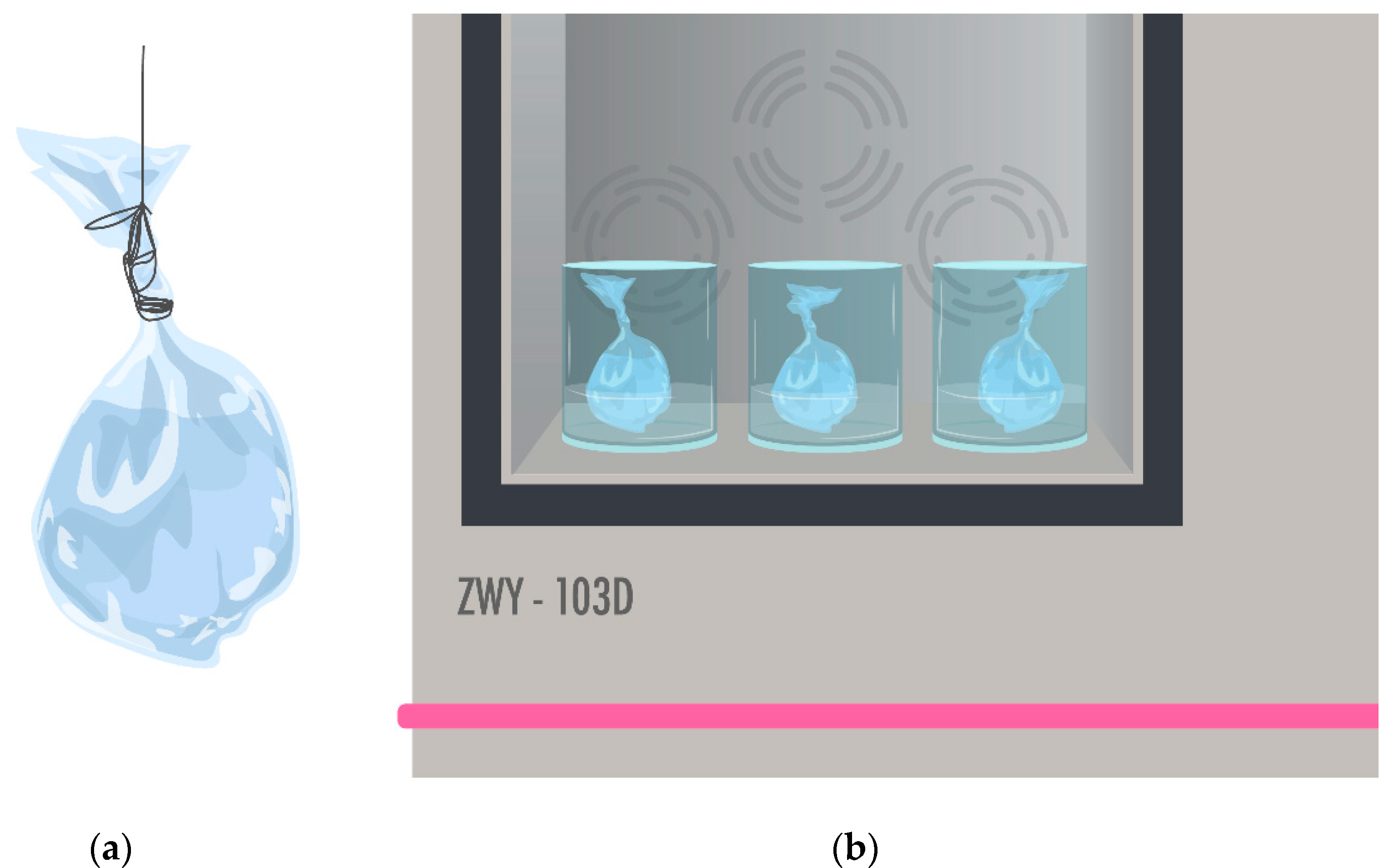
(a) Dialysis tubing with MA/EA NP suspension to evaluate glibenclamide release; (b) Shaker-incubator with dialysis tubing in PBS pH 7.4 solution.
Figure 1.
(a) Dialysis tubing with MA/EA NP suspension to evaluate glibenclamide release; (b) Shaker-incubator with dialysis tubing in PBS pH 7.4 solution.
Figure 2.
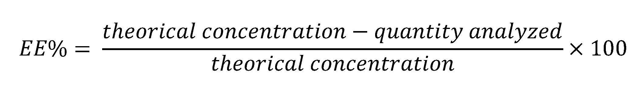
Encapsulation efficiency equation.
Figure 2.
Encapsulation efficiency equation.
Figure 3.
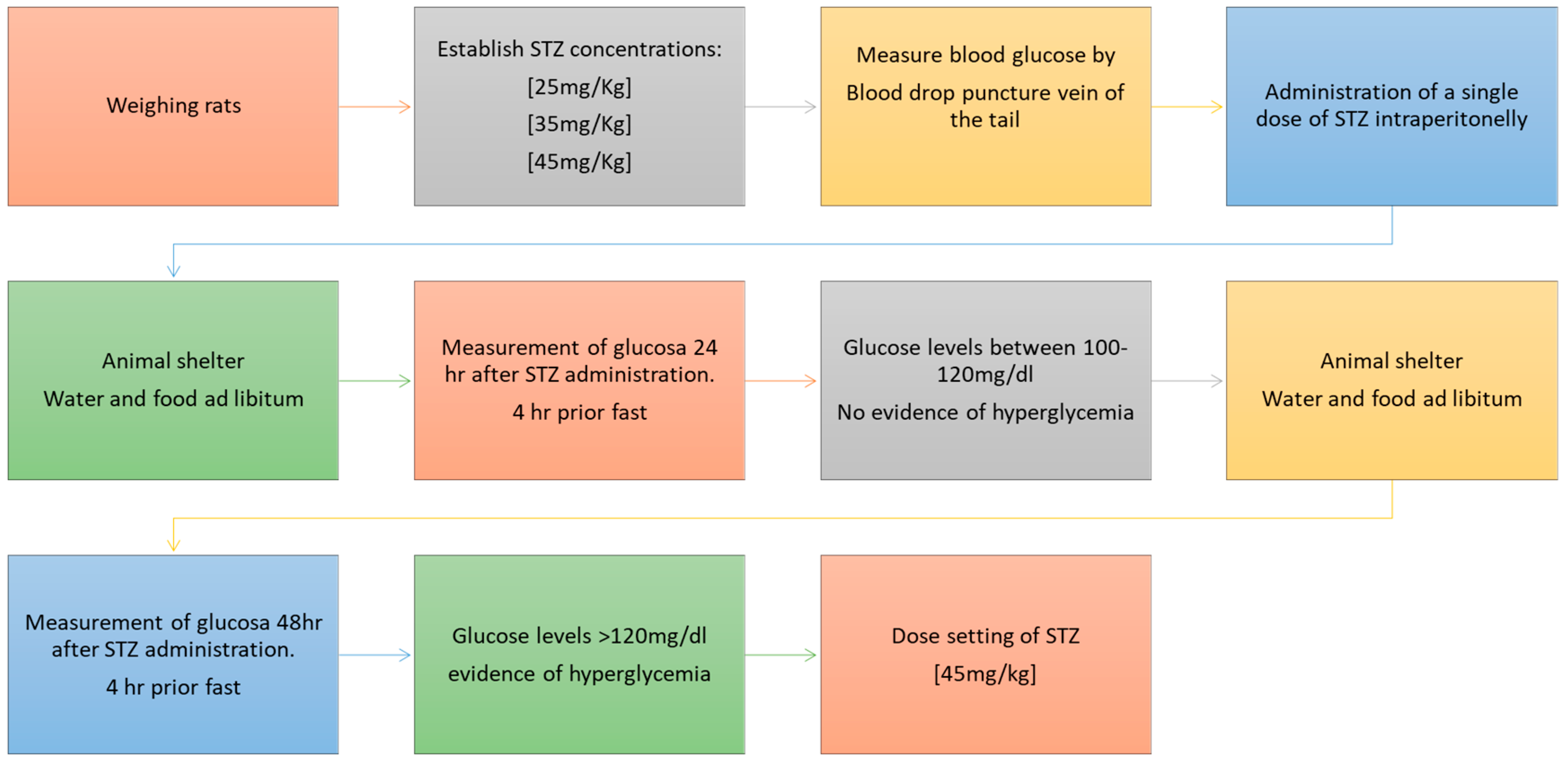
Selection of the dose of STZ to generate hyperglycemia in rats.
Figure 3.
Selection of the dose of STZ to generate hyperglycemia in rats.
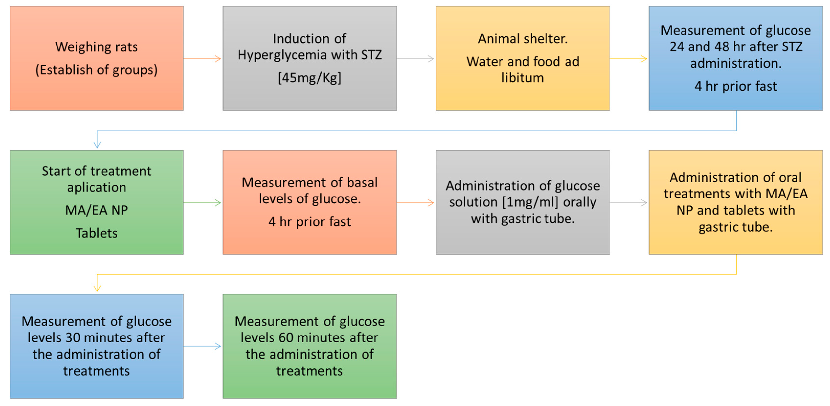
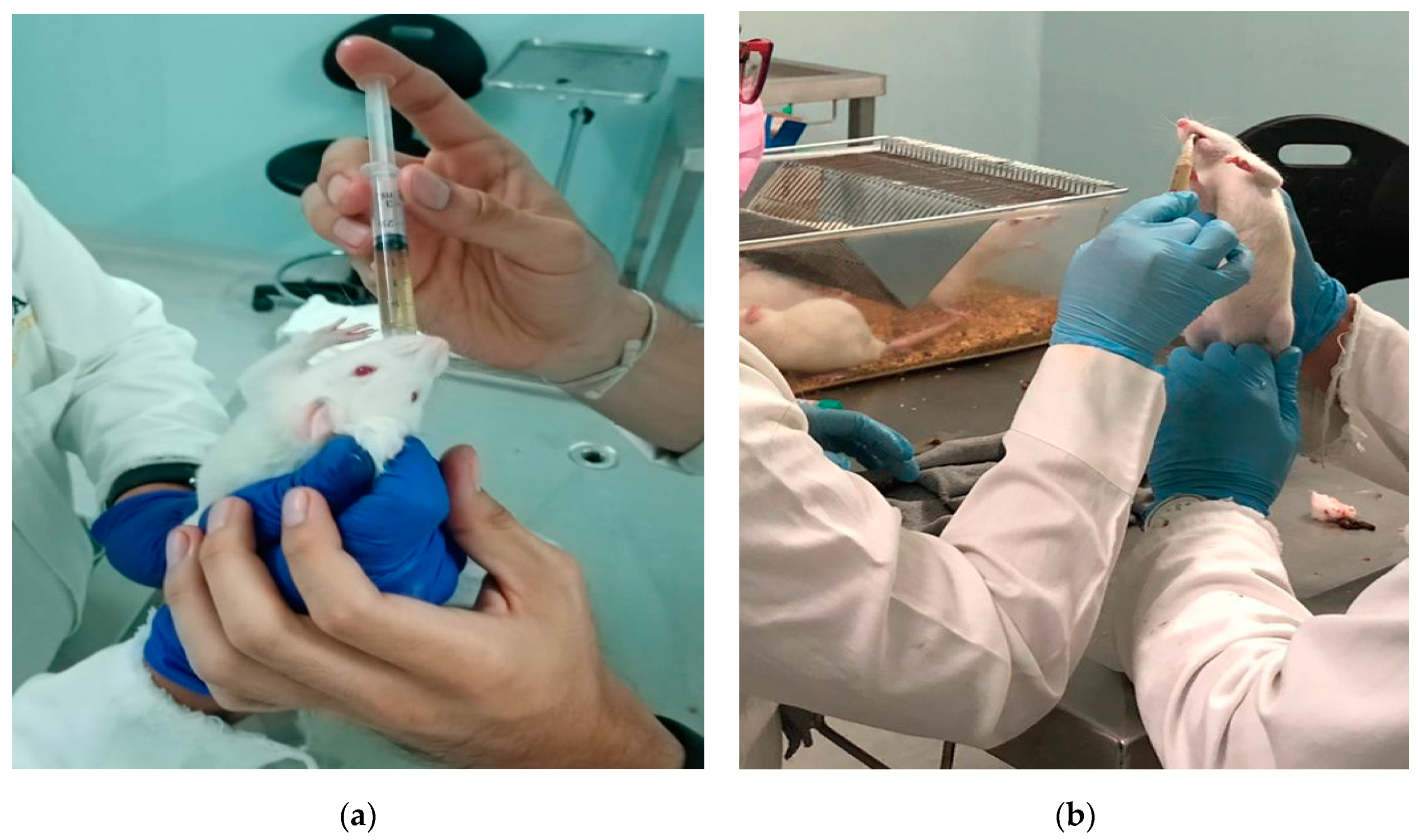
Figure 4.
Application of treatments and determination of blood glucose levels.
Figure 4.
Application of treatments and determination of blood glucose levels.
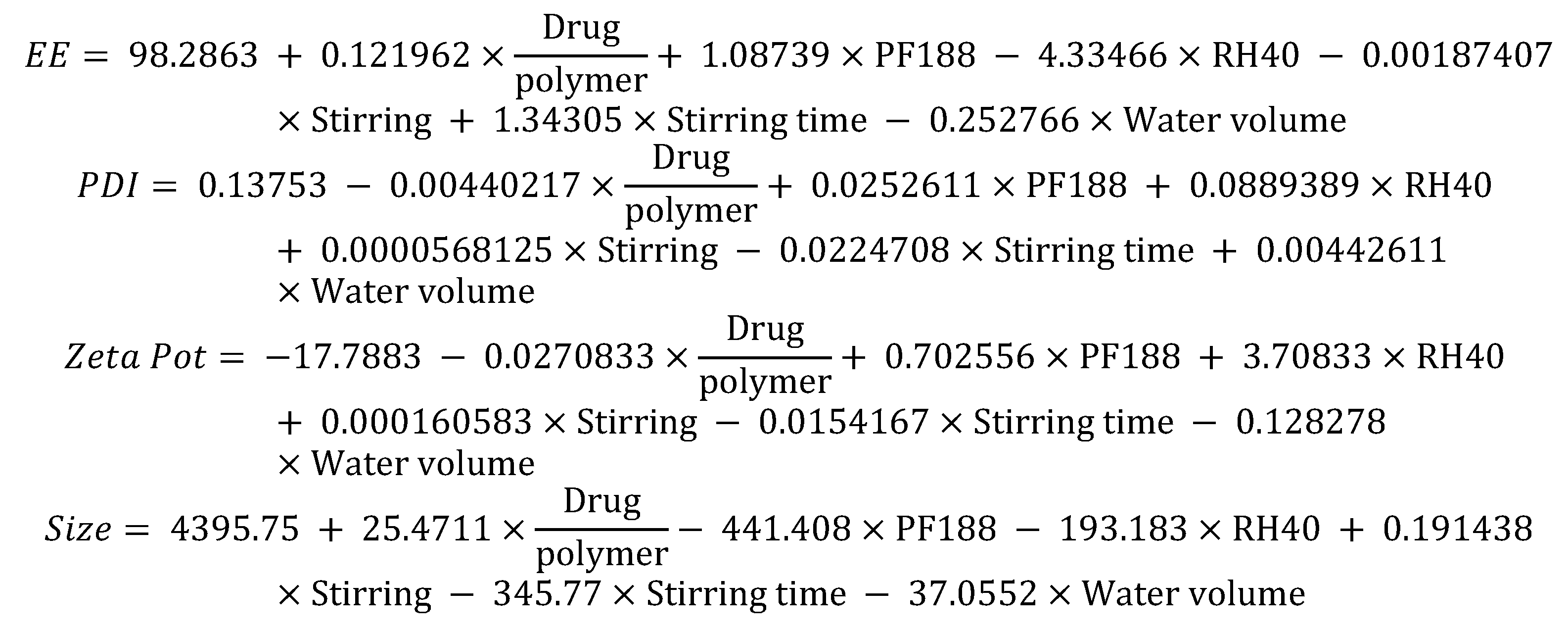
Figure 5.
Equations showing the interactions of the different factors in the development of NPs in the screening phase.
Figure 5.
Equations showing the interactions of the different factors in the development of NPs in the screening phase.
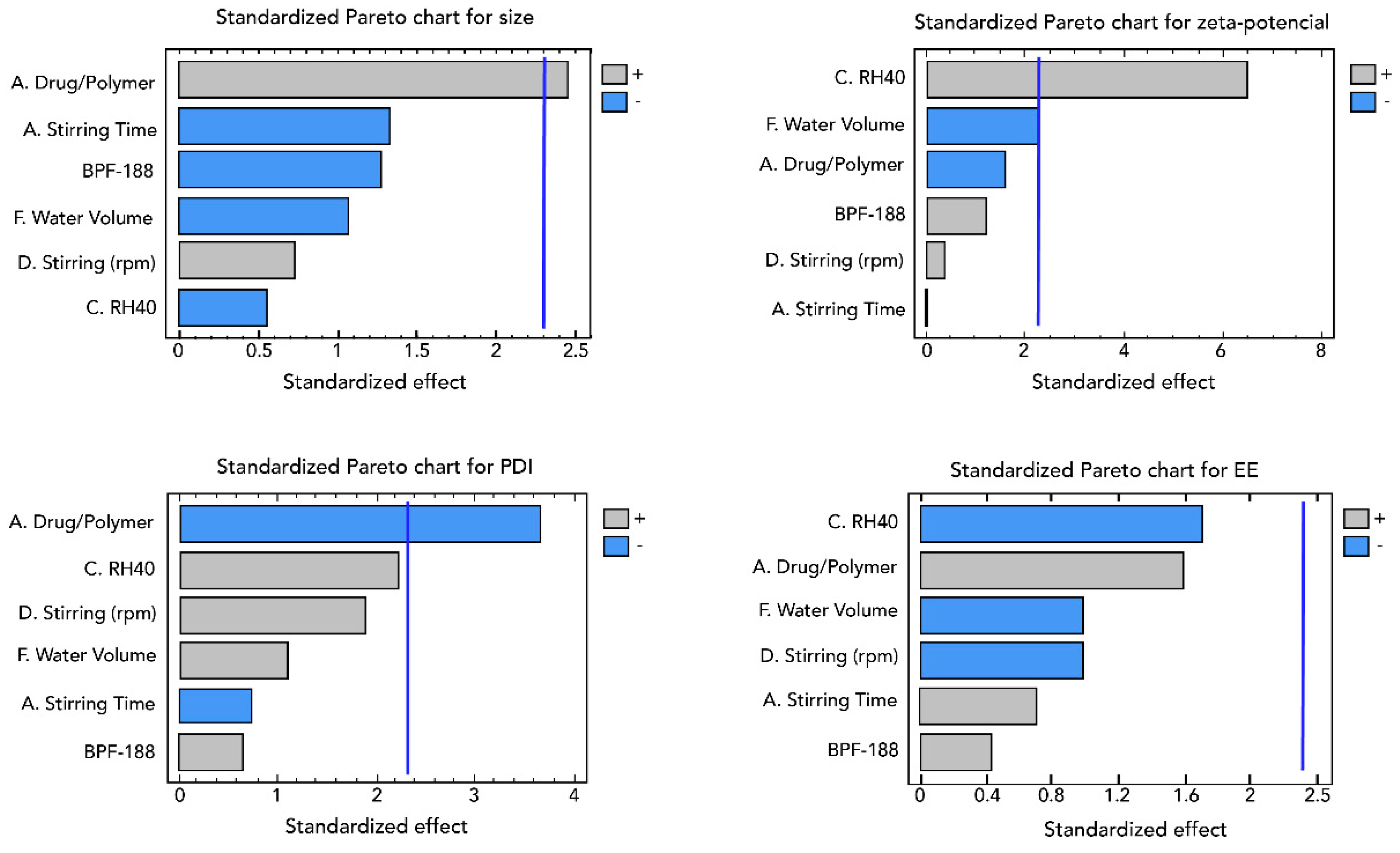
Figure 6.
Pareto diagrams showing the factors with significant response in the screening design for the synthesis of NPs with glibenclamide.
Figure 6.
Pareto diagrams showing the factors with significant response in the screening design for the synthesis of NPs with glibenclamide.
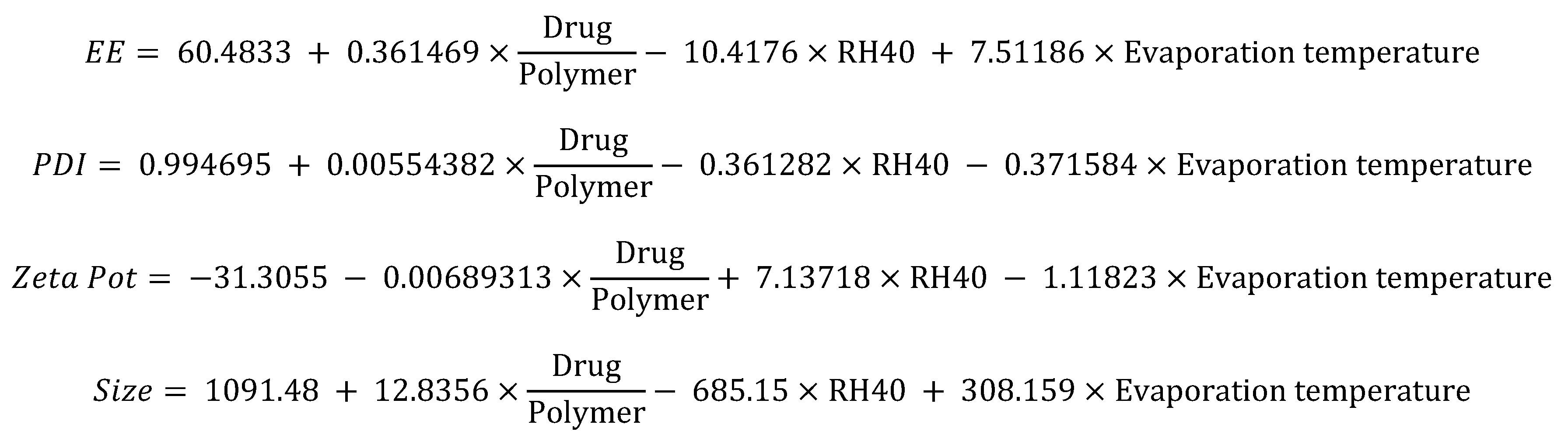
Figure 7.
Interaction between factors for any response in the optimization phase.
Figure 7.
Interaction between factors for any response in the optimization phase.
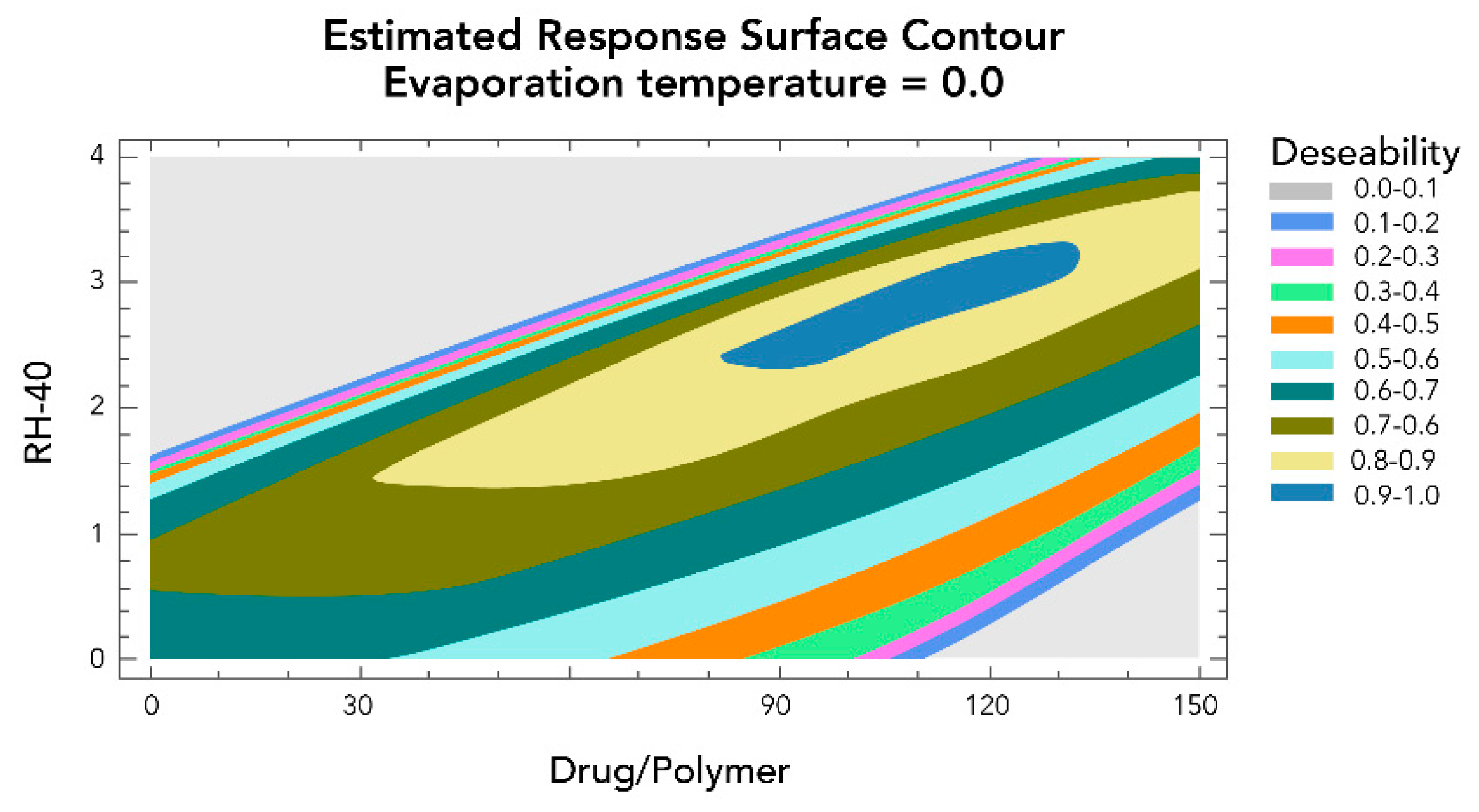
Figure 8.
Response surface plot for the development of nanoparticles of 50 nm in diameter.
Figure 8.
Response surface plot for the development of nanoparticles of 50 nm in diameter.
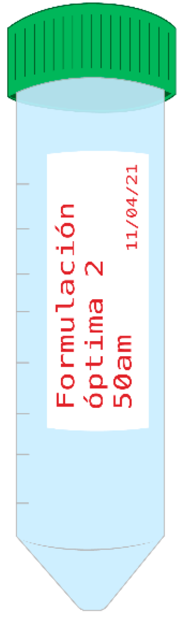
Figure 9.
Formulation of optimized glibenclamide NPs.
Figure 9.
Formulation of optimized glibenclamide NPs.
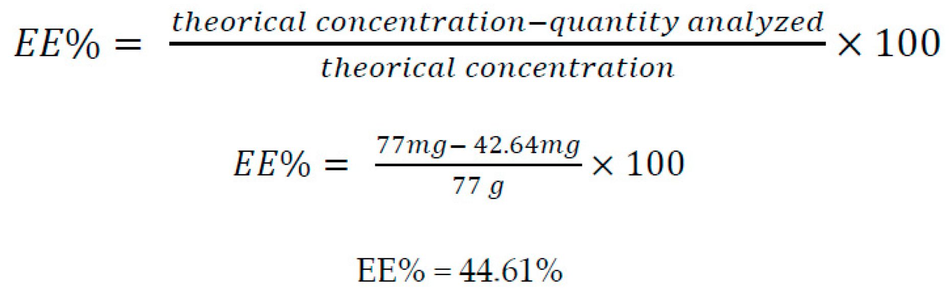
Figure 10.
Equation substituted with units to obtain the encapsulation efficiency.
Figure 10.
Equation substituted with units to obtain the encapsulation efficiency.
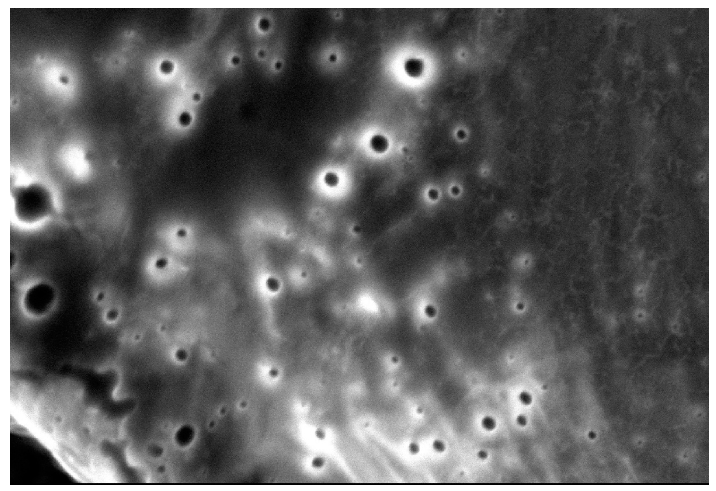
Figure 11.
SEM of the optimized formulation of MA/EA copolymer NPs loaded with glibenclamide, size 19nm magnification 2500×.
Figure 11.
SEM of the optimized formulation of MA/EA copolymer NPs loaded with glibenclamide, size 19nm magnification 2500×.
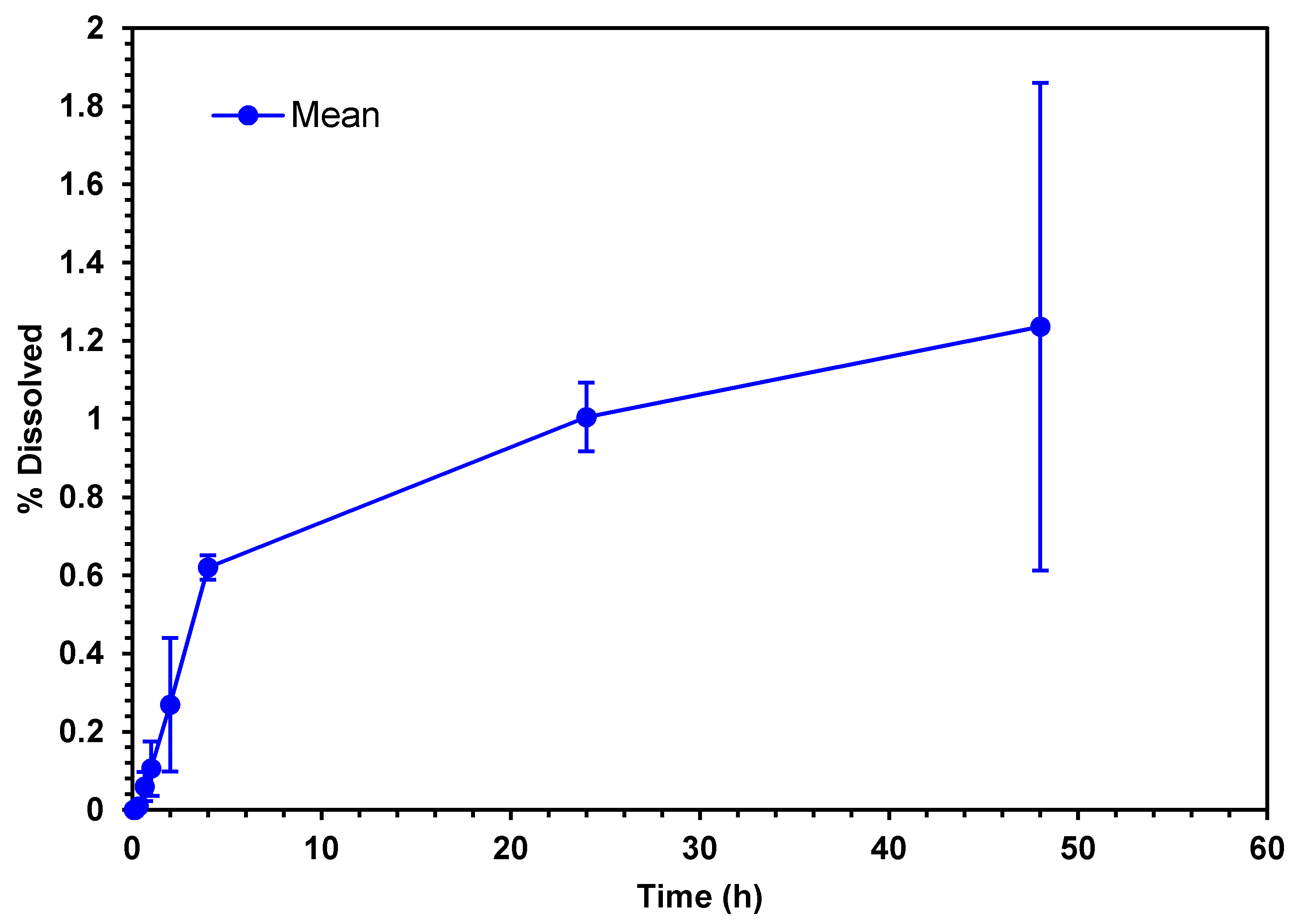
Figure 12.
Drug release profiles of the optimized formulation of MA/EA NPs in dialysis tubing bags.
Figure 12.
Drug release profiles of the optimized formulation of MA/EA NPs in dialysis tubing bags.
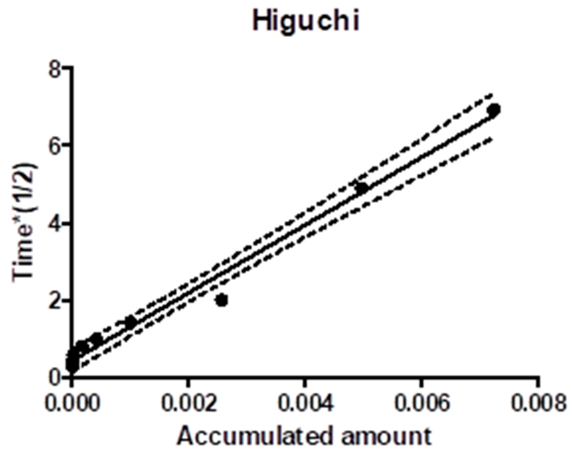
Figure 13.
Higuchi model where r2 = 0.9850.
Figure 13.
Higuchi model where r2 = 0.9850.
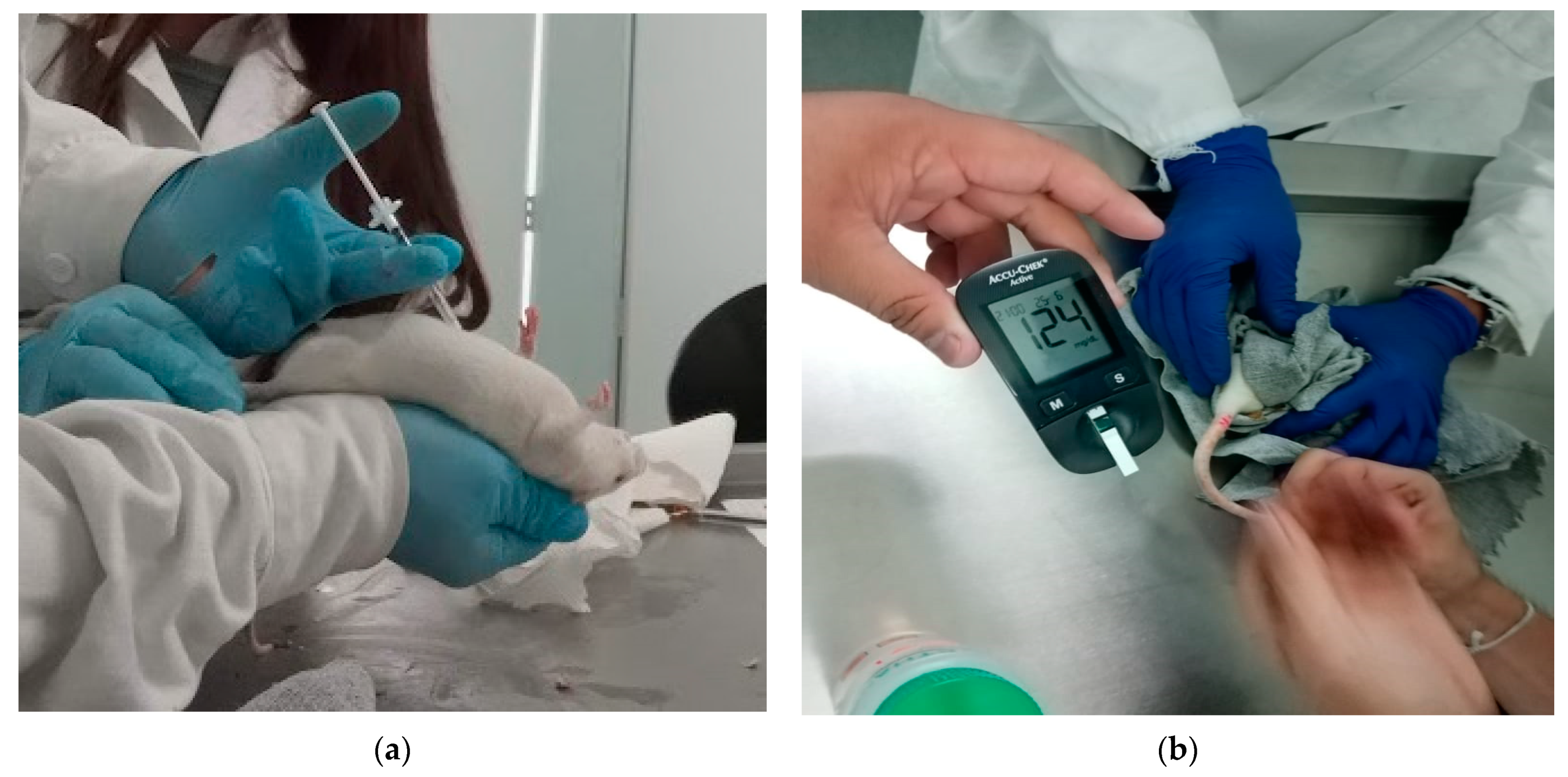
Figure 14.
(a) STZ administration through the intraperitoneal. (b) Glucose levels greater that 120 mg/dL are indicative of animals with diabetes.
Figure 14.
(a) STZ administration through the intraperitoneal. (b) Glucose levels greater that 120 mg/dL are indicative of animals with diabetes.
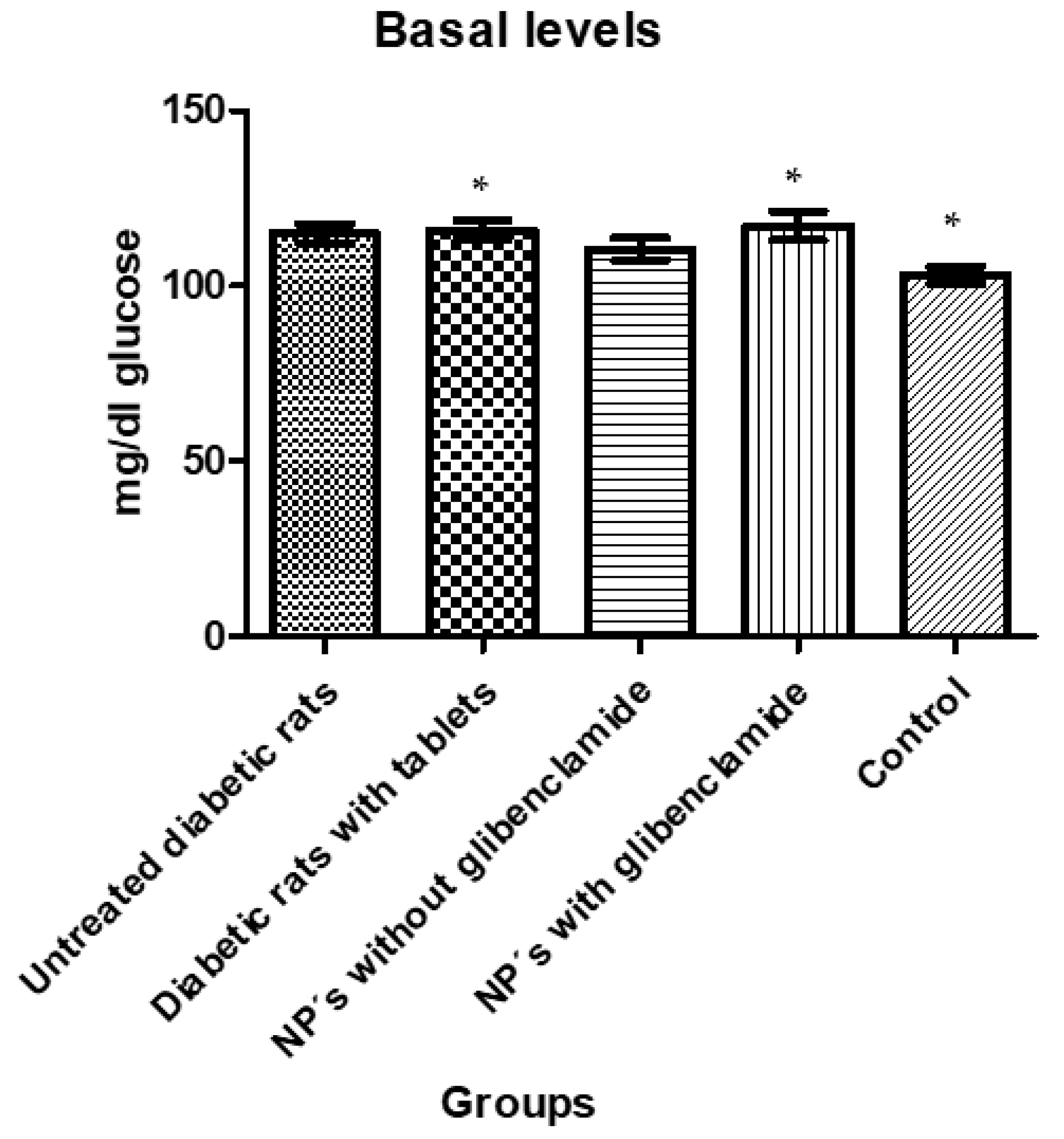
Figure 15.
Baselines glucose levels showing significant differences between groups. The asterisks (*) represent a statistically significant difference between groups (p < 0.05).
Figure 15.
Baselines glucose levels showing significant differences between groups. The asterisks (*) represent a statistically significant difference between groups (p < 0.05).
Figure 16.
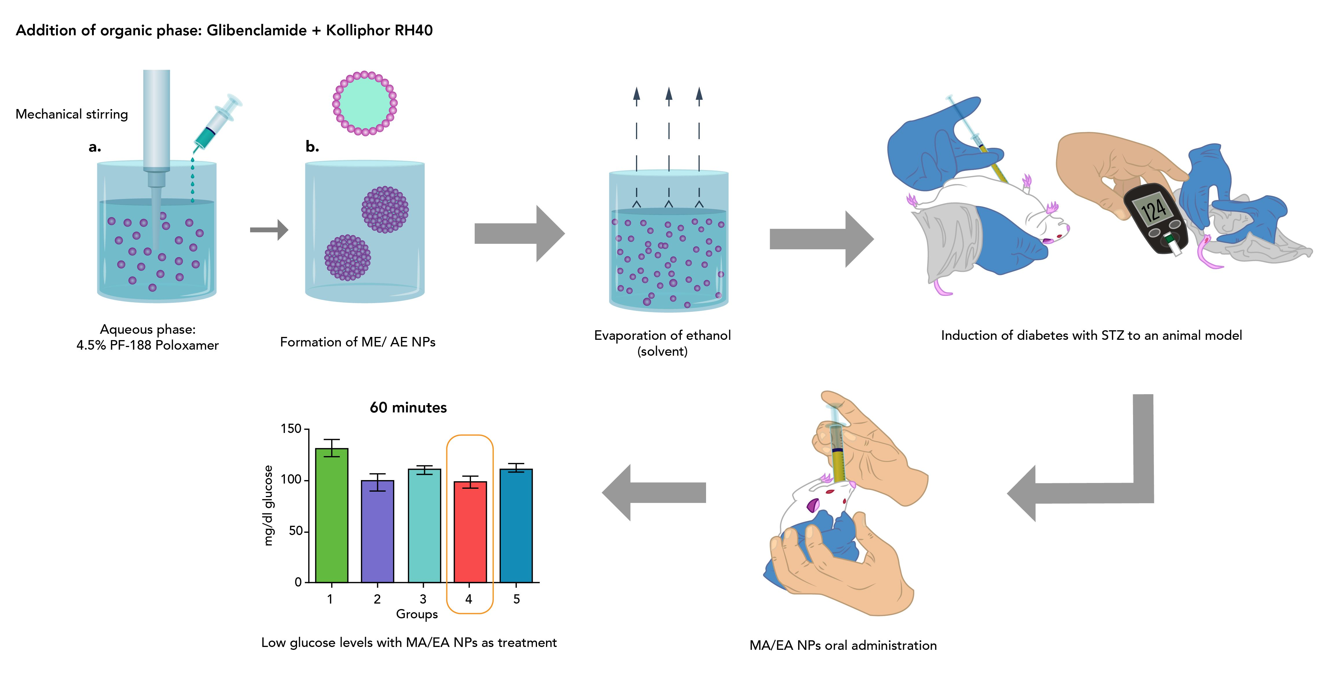
(a) Oral administration of glucose solution (1 g/mL). (b) Oral administration of MA/EA NPs suspension.
Figure 16.
(a) Oral administration of glucose solution (1 g/mL). (b) Oral administration of MA/EA NPs suspension.
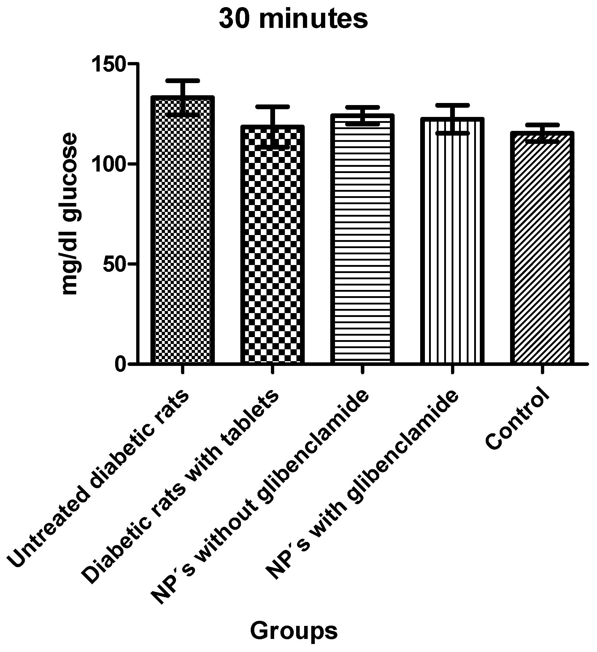
Figure 17.
Glucose levels 30 min after administration of a glucose solution and glibenclamide treatments.
Figure 17.
Glucose levels 30 min after administration of a glucose solution and glibenclamide treatments.
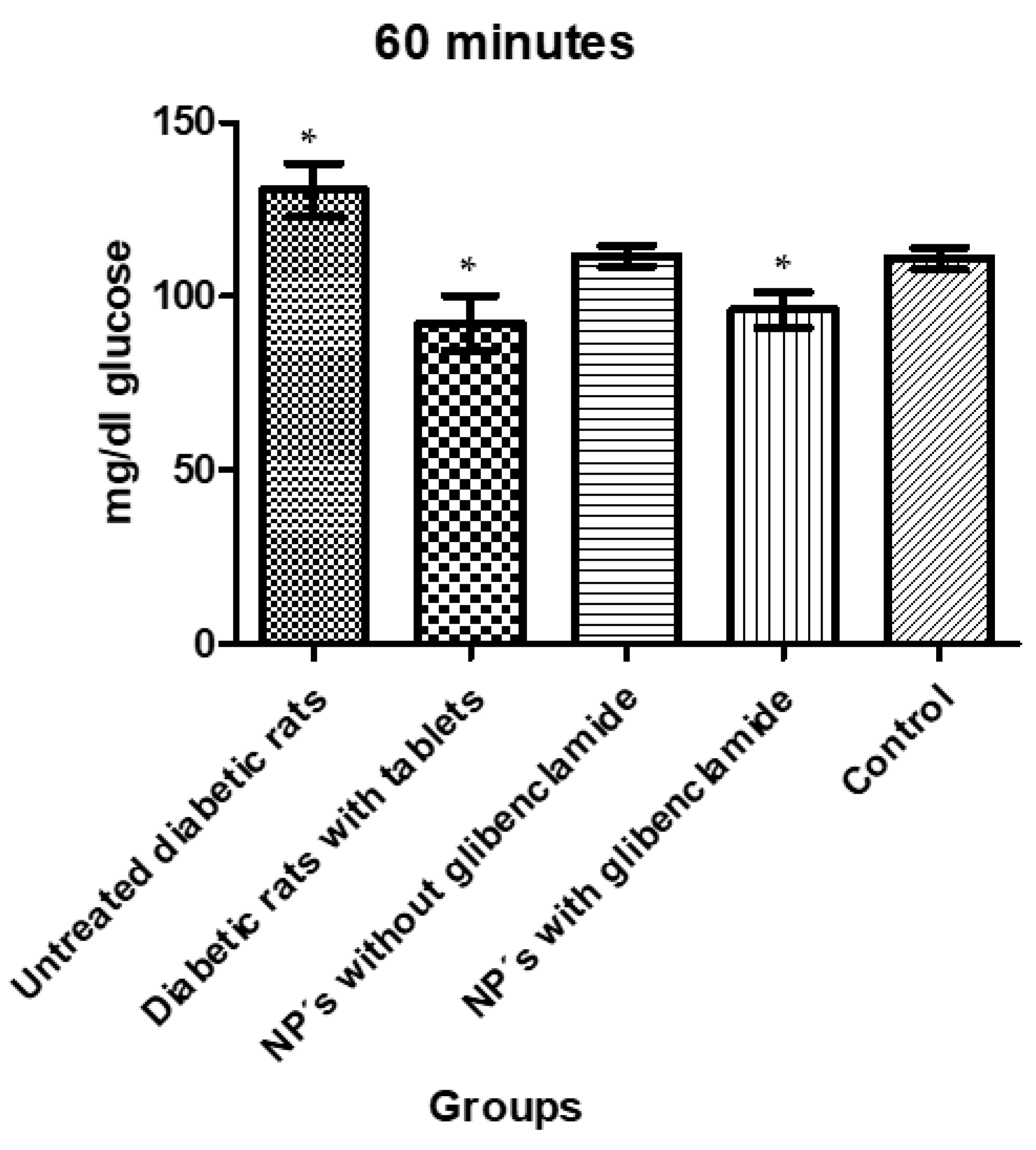
Figure 18.
Glucose levels 60 min after administration of a glucose solution and glibenclamide treatments. The asterisks (*) represent a statistically significant difference between groups (p < 0.05).
Figure 18.
Glucose levels 60 min after administration of a glucose solution and glibenclamide treatments. The asterisks (*) represent a statistically significant difference between groups (p < 0.05).
Table 1.
Independent variables and levels selected for the screening design.
Table 1.
Independent variables and levels selected for the screening design.
| Factors | Low | High | Units |
|---|
| Drug/polymer | 50 | 150 | Mg |
| PF-188 | 1.5 | 4.5 | % |
| RH-40 | 1.5 | 4.5 | G |
| Stirring speed | 2000 | 6000 | Rpm |
| Stirring time | 2.0 | 6.0 | Min |
| Volume of water | 45 | 75 | mL |
Table 2.
Dependent variables selected in the optimization phase.
Table 2.
Dependent variables selected in the optimization phase.
| Response | Units |
|---|
| Size | Nm |
| Zeta potential | mV |
| PDI | -- |
| Encapsulation efficiency (EE) | % |
Table 3.
Independent variables in the optimization of glibenclamide ME/EA NPs.
Table 3.
Independent variables in the optimization of glibenclamide ME/EA NPs.
| Factors | Low | High | Units | Continuous |
|---|
| Drug/Polymer | 40 | 120 | mg | Yes |
| RH-40 | 1 | 3 | g | Yes |
| Evaporation temperature | −1 | 1 | °C | Yes |
Table 4.
Dependent variables in the optimization phase.
Table 4.
Dependent variables in the optimization phase.
| Response | Units |
|---|
| Size | Nm |
| Zeta potential | mV |
| PDI | -- |
| EE | % |
Table 5.
Group in which the 25 rats were classified by weight order.
Table 5.
Group in which the 25 rats were classified by weight order.
| Animals Were Divided into 5 Different Groups with 5 Individuals Each as Follows: |
|---|
| Group 1: untreated diabetic rats |
| Group 2: diabetic rats with conventional pharmaceutical form (tablets) |
| Group 3: diabetic rats administered with NP without glibenclamide |
| Group 4: diabetic rats administered with NP with glibenclamide |
| Group 5: control |
Table 6.
Factors and responses in the screening phase.
Table 6.
Factors and responses in the screening phase.
| Drug/Polymer | PF-188 | Kolliphor RH-40® | Stirring | Stirring Time | Water Volume | Size | Zeta Pot | PDI | EE |
|---|
| mg | % | G | rpm | min | mL | Nm | mV | | % |
| 50 | 4.5 | 4.5 | 6000 | 2 | 75 | 24.59 | −11.42 | 1.2 | 75.253666 |
| 150 | 1.5 | 4.5 | 6000 | 2 | 75 | 4687 | −10.14 | 0.2939 | 63.397299 |
| 150 | 4.5 | 1.5 | 6000 | 6 | 45 | 3891 | −16.22 | 0.1027 | 99.312885 |
| 50 | 1.5 | 1.5 | 6000 | 6 | 75 | 1634 | −23.44 | 0.4802 | 87.46687 |
| 150 | 1.5 | 4.5 | 2000 | 2 | 45 | 5117 | −11.54 | 0.189 | 94.337278 |
| 150 | 4.5 | 1.5 | 6000 | 2 | 45 | 3664 | −20.68 | 0.2228 | 98.847868 |
| 100 | 3 | 3 | 4000 | 4 | 60 | 5136 | −10.69 | 0.3943 | 97.082929 |
| 150 | 4.5 | 4.5 | 2000 | 6 | 75 | 14.79 | −11.54 | 0.4279 | 88.191434 |
| 150 | 1.5 | 1.5 | 2000 | 6 | 75 | 1893 | −27 | 0.0299 | 101.33701 |
| 50 | 1.5 | 1.5 | 2000 | 2 | 45 | 2245 | −18.03 | 0.3975 | 90.442499 |
| 50 | 4.5 | 1.5 | 2000 | 2 | 75 | 37.11 | −17 | 0.5533 | 70.439951 |
| 100 | 3 | 3 | 4000 | 4 | 60 | 4577 | −14.36 | 0.7203 | 74.129591 |
| 50 | 1.5 | 4.5 | 6000 | 6 | 45 | 22.13 | −5.168 | 0.969 | 62.067704 |
| 100 | 3 | 3 | 4000 | 4 | 60 | 12.74 | −12.66 | 0.3544 | 62.876815 |
| 50 | 4.5 | 4.5 | 2000 | 6 | 45 | 21.3 | −5.812 | 0.3075 | 86.575837 |
Table 7.
Factors and responses established for optimization design.
Table 7.
Factors and responses established for optimization design.
| Block | Drug/Polymer | Kolliphor RH-40® | Evaporation Temperature | Size | Zeta Potential | PDI | EE |
|---|
| | Mg | G | °C | nm | mV | | % |
| 1 | 40 | 1 | 1 | 1565 | −18.19 | 0.6814 | 79.491841 |
| 1 | 80 | 2 | 1.68179 | 756 | −18.93 | 0.6576 | 83.9436238 |
| 1 | 120 | 1 | −1 | 1823 | −24.94 | 4.418 | 93.0083276 |
| 1 | 80 | 3.68179 | 0 | 13.97 | −13.35 | 0.2083 | 76.8001864 |
| 1 | 147.272 | 2 | 0 | 1250 | −17.75 | 0.3323 | 80.6717907 |
| 1 | 120 | 1 | 1 | 3979 | −25.41 | 0.04271 | 94.2851601 |
| 1 | 80 | 2 | 0 | 34.43 | −13.67 | 0.3513 | 47.9191043 |
| 1 | 40 | 1 | −1 | 32.4 | −23.82 | 1.374 | 79.6281078 |
| 1 | 120 | 3 | −1 | 746 | 0.02799 | 0.9255 | 88.8181854 |
| 1 | 120 | 3 | 1 | 22.02 | −13.71 | 0.4585 | 87.1761386 |
| 1 | 80 | 2 | −1.68179 | 15.83 | −15.17 | 0.3648 | 10.3197805 |
| 1 | 80 | 2 | 0 | 27.75 | −18.33 | 0.08396 | 63.2713165 |
| 1 | 40 | 3 | −1 | 15.93 | −12.29 | 0.3544 | 43.862202 |
| 1 | 12.7283 | 2 | 0 | 19.16 | −13.77 | 0.3824 | 44.8243383 |
| 1 | 40 | 3 | 1 | 14.97 | −12.66 | 0.3222 | 23.1320136 |
| 1 | 80 | 0.318207 | 0 | 1653 | −39.36 | 0.4928 | 99.8984444 |
Table 8.
Size, PDI, and zeta potential of the optimal MA/EA NP formulation.
Table 8.
Size, PDI, and zeta potential of the optimal MA/EA NP formulation.
| Expected Size | Size (nm) | PDI | Zeta Potential |
|---|
| 50 nm | 18.98 +/− 9.14 | 0.37085 +/− 0.014 | −13.7125 +/− 1.82 |
Table 9.
Load capacity and encapsulation efficiency of methacrylic acid–ethyl acrylate copolymer nanoparticles.
Table 9.
Load capacity and encapsulation efficiency of methacrylic acid–ethyl acrylate copolymer nanoparticles.
| Absorbance 305 nm | Dilution | Quantification (µg/mL) | Dilution Factor | Quantification (mg) | Theoretical Load (mg) | Load Capacity (mg) | Encapsulation Efficiency (%) |
|---|
1.4907
1.4865
1.4907 | (1:2) | 251.118644 | 502.237288 | 42.6901695 | 77 | 34.3098305 | 44.5582214 |
| (1:2) | 250.40678 | 500.813559 | 42.5691525 | 77 | 34.4308475 | 44.7153863 |
| (1:2) | 251.118644 | 502.237288 | 42.6901695 | 77 | 34.3098305 | 44.5582214 |
| 1.4893 | (1:2) | 250.881356 | 501.762712 | 42.6498305 | 77 | 34.3501695 | 44.61 +/- 0.22 |
Table 10.
Tukey test showing the groups that showed a statistically significant difference in baseline levels.
Table 10.
Tukey test showing the groups that showed a statistically significant difference in baseline levels.
| Tukey’s Multiple Comparison Test | Significant p < 0.05 | Summary | 95% CI of diff |
|---|
| Group 1 vs. Group 2 | No | ns | −13.78 to 12.00 |
| Group 1 vs. Group 3 | No | ns | −8.380 to 17.40 |
| Group 1 vs. Group 4 | No | ns | −15.03 to 10.75 |
| Group 1 vs. Group 5 | No | ns | −0.9797 to 24.80 |
| Group 2 vs. Group 3 | No | ns | −6.755 to 17.55 |
| Group 2 vs. Group 4 | No | ns | −13.40 to 10.90 |
| Group 2 vs. Group 5 | Yes | * | 0.6451 to 24.95 |
| Group 3 vs. Group 4 | No | ns | −18.80 to 5.505 |
| Group 3 vs. Group 5 | No | ns | −4.755 to 19.55 |
| Group 4 vs. Group 5 | Yes | * | 1.895 to 26.20 |
Table 11.
Tukey test showing the groups that showed a statistically significant difference at 60 min.
Table 11.
Tukey test showing the groups that showed a statistically significant difference at 60 min.
| Tukey’s Multiple Comparison Test | Significant p < 0.05 | Summary | 95% CI of diff |
|---|
| Group 1 vs. Group 2 | Yes | *** | 15.42 to 61.18 |
| Group 1 vs. Group 3 | No | ns | −4.005 to 41.76 |
| Group 1 vs. Group 4 | Yes | *** | 11.52 to 57.29 |
| Group 1 vs. Group 5 | No | ns | −3.008 to 42.23 |
| Group 2 vs. Group 3 | No | ns | −41.30 to 2.460 |
| Group 2 vs. Group 4 | No | ns | −25.78 to 17.99 |
| Group 2 vs. Group 5 | No | ns | −40.29 to 2.919 |
| Group 3 vs. Group 4 | No | ns | −6.354 to 37.41 |
| Group 3 vs. Group 5 | No | ns | −20.87 to 22.34 |
| Group 4 vs. Group 5 | No | ns | −36.40 to 6.813 |


 ,
, 


