A Comprehensive Brain MRI Image Segmentation System Based on Contourlet Transform and Deep Neural Networks

Abstract

Brain tumors are one of the deadliest types of cancer. Rapid and accurate identification of brain tumors, followed by appropriate surgical intervention or chemotherapy, increases the probability of survival. Accurate determination of brain tumors in MRI scans determines the exact location of surgical intervention or chemotherapy. However, this accurate segmentation of brain tumors, due to their diverse morphologies in MRI scans, poses challenges that require significant expertise and accuracy in image interpretation. Despite significant advances in this field, there are several barriers to proper data collection, particularly in the medical sciences, due to concerns about the confidentiality of patient information. However, research papers for learning systems and proposed networks often rely on standardized datasets because a specific approach is unavailable. This system combines unsupervised learning in the adversarial generative network component with supervised learning in segmentation networks. The system is fully automated and can be applied to tumor segmentation on various datasets, including those with sparse data. In order to improve the learning process, the brain MRI segmentation network is trained using a generative adversarial network to increase the number of images. The U-Net model was employed during the segmentation step to combine the remaining blocks efficiently. Contourlet transform produces the ground truth for each MRI image obtained from the adversarial generator network and the original images in the processing and mask preparation phase. On the part of the adversarial generator network, high-quality images are produced, the results of which are similar to the histogram of the original images. Finally, this system improves the image segmentation performance by combining the remaining blocks with the U-net network. Segmentation is evaluated using brain magnetic resonance images obtained from Istanbul Medipol Hospital. The results show that the proposed method and image segmentation network, which incorporates several criteria, such as the DICE criterion of 0.9434, can be effectively used in any dataset as a fully automatic system for segmenting different brain MRI images.

1. Introduction

Brain cancer is a highly lethal type of cancer, and an immediate and precise diagnosis will significantly affect a patient’s chances of survival. A brain tumor is formed by any cluster of aberrant cells that occupy space within the brain. Over 40 distinct classifications of brain tumors have been identified so far, categorized into two broad groups, Benign tumors exhibit slow growth and do not metastasize. Malignant tumors are malignant neoplasms characterized by uncontrolled growth and the potential to metastasize to other regions of the brain and spinal cord [1,2,3]. Multiple therapeutic alternatives are available for individuals diagnosed with brain tumors. Some of these techniques include surgery, radiation, and chemotherapy.

Precise localization of malignancy is crucial for performing surgery on individuals with brain tumors and enhancing their chances of survival. Segmenting the brain before surgery based on tumor size, shape, position, and light dispersion is complex [4]. Computed tomography (CT) or magnetic resonance imaging (MRI) are used to assess the dimensions and location of tumors in all three treatment approaches. Typically, medical professionals, such as doctors and radiologists, examine brain tumors. Radiologists commonly employ MRI sequences and compare these images to identify brain tumor locations accurately [5]. Nevertheless, manually evaluating and segmenting MRI data is intricate and time-consuming. Numerous techniques have been suggested to determine the precise location of the tumor, in order to minimize human mistakes and enhance precision, by progresses in computer technology, each yielding distinct outcomes.

The advancements in deep learning in medical domains, along with the advancements in graphics cards and processors in recent years [6,7,8,9], have led to significant improvements in the performance of deep learning networks. The improvement is so significant that performance exceeds human knowledge in specific medical applications, such as diagnostics [10,11]. This successfully addresses challenges related to distinct attributes of images, including variations in size, shape, location, intensity, unclear borders, and contradicting properties observed in diverse imaging [12]. Nevertheless, this research encountered particular challenges, such as the absence of standardized data and the scattered nature of the available data, which consisted of many sets. Additionally, the time-consuming processing and preparation of this data using various software tools prompted the adoption of a method for segmenting brain tumor regions.

This study includes Section 2 and Section 3, including data preparation and pre-processing, followed by GAN networks for data enrichment. To train the segmentation network, we prepared the images for the background truth using the contourlet transform. Finally, we segmented the images by combining a remaining block in the segmentation network. In the last part, we analyze the results and explain them.

2. Literature Review

In recent years, extensive studies have been conducted on the importance of brain cancer, accurate localization and tumor dimensions, due to the proliferation of deep networks. Several of these articles focus on the diagnosis and classification of brain tumors. Other papers prioritize segmentation, while some papers deal with the basic design of the network and ways to enhance it. A few articles also produce new data, summarizing the work done.

The authors in [13] have used standard data to diagnose glioma and automatically segment three-dimensional brain tumors. The proposed model combines a deep residual network and a U-Net model and thus uses low-level and high-level features for prediction. The proposed architecture is applied to the mean DICE score for tumor core (TC), total tumor (WT), and tumor enhancement (ET) in the BraTS 2020 dataset.

In [14], a technique is employed to identify and segment brain images. This structure has used fast demarcation methods and thresholding methods for segmentation. The classification section examines the use of two pre-trained networks, VGG-19 and AlexNet, in conjunction with a transfer learning technique to classify MR images. For this purpose, Kegel and Figshare datasets were used.

In [15], the authors proposed a semantic segmentation approach utilizing a convolutional neural network that employs the encoder and decoder techniques. This method is designed to automatically segment brain tumors on a 3D brain tumor segmentation BraTS image dataset. The dataset comprises images captured using four imaging methods. This technique effectively measured the tumor’s area and dimensions, including its height, width, and depth. Additionally, it generated images of various planes, such as sagittal, coronal, and axial. Ultimately, the dice criterion was employed to assess this network.

In [16], the U-Net model, a technique for image segmentation, was used. The suggested methodology incorporates jump connections, two twisting sequences of metro asymmetry, and a unique residual path called the Multipath residual attention block, which was put into the system. This study utilized the brain tumor segmentation challenge datasets from 2018 to 2021.

In [17], a new automatic technique for brain tumor segmentation based on the U network was developed using a multiscale residual attention approach. This approach allows changes in the specific area of focus to be implemented, increasing accuracy in identifying the tumor’s location. The proposed technique for brain tumor segmentation is evaluated using BraTS2020 data.

In [18], the authors created a sophisticated 3D residual neural network specifically designed to identify and separate brain tumors accurately. This approach employs the BraTS 2018 dataset and demonstrates decreased computational complexity and GPU memory utilization.

In [8], the authors devised an automated segmentation technique employing a convolutional neural network (CNN) deep neural network architecture. The authors used 3 × 3 small kernels for a deeper architecture design. The research findings in the 2013 segmentation challenge were evaluated using BraTS 2013 based on the dice criteria.

In [19], the authors have used the transfer learning technique in a deep neural network using the complex ResNet34 architecture. After that, this model was used to automatically classify MRI images into two distinct groups: normal brain and brain with pathological condition. During training, the network used techniques such as fine-tuning, determining the best learning rate, and traditional data augmentation. The entire study was based on 613 images from the Harvard University website.

In [20], the Fusion of CNN and BAT networks was applied to different MRI input images to detect human brain tumors. First, they were processed to identify and reduce any background noise. The utilization of a 2D Gabor filter resulted in enhanced precision in identifying tumors. Despite being limited to a small dataset obtained from the hospital, the proposed method was successful. It was evaluated based only on the collected data and with the Dice criterion.

In [21], a novel deep-learning approach is introduced for classifying tumors in MR images. The method utilizes a discriminant within a generative adversarial network to extract reliable features and understand the structure of MR images using convolutional layers. The approach was applied to various datasets of MR images. The model was trained, after which the fully connected layers were substituted, and the entire deep network was further trained as a classifier to identify the three tumor types accurately. The method was used for an MRI data set consisting of 233 individuals diagnosed with three distinct forms of brain tumor: meningioma, glioma, and pituitary tumor. The performance of the network was assessed using evaluation parameters, such as F1 score, sensitivity, and accuracy.

The review of sources and articles shows that the preparing of desired data and MR images is still one of the challenges and issues facing deep learning networks, especially in segmentation methods. Given that segmentation is part of supervised learning, we need labeling. For this purpose, a background truth (mask) must be prepared for each image, which takes time and requires skill. For this reason, most papers have used standard datasets, such as the Brain Tumor Segmentation Challenge dataset (BraTS), Kaggle dataset, or Figshare dataset, for deep learning segmentation methods or their data in the classification section.

3. Method

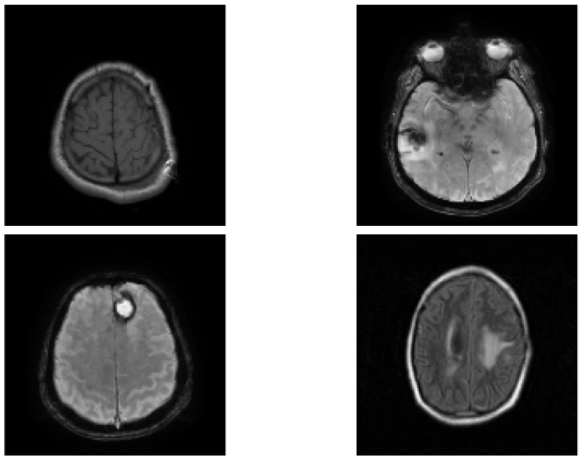
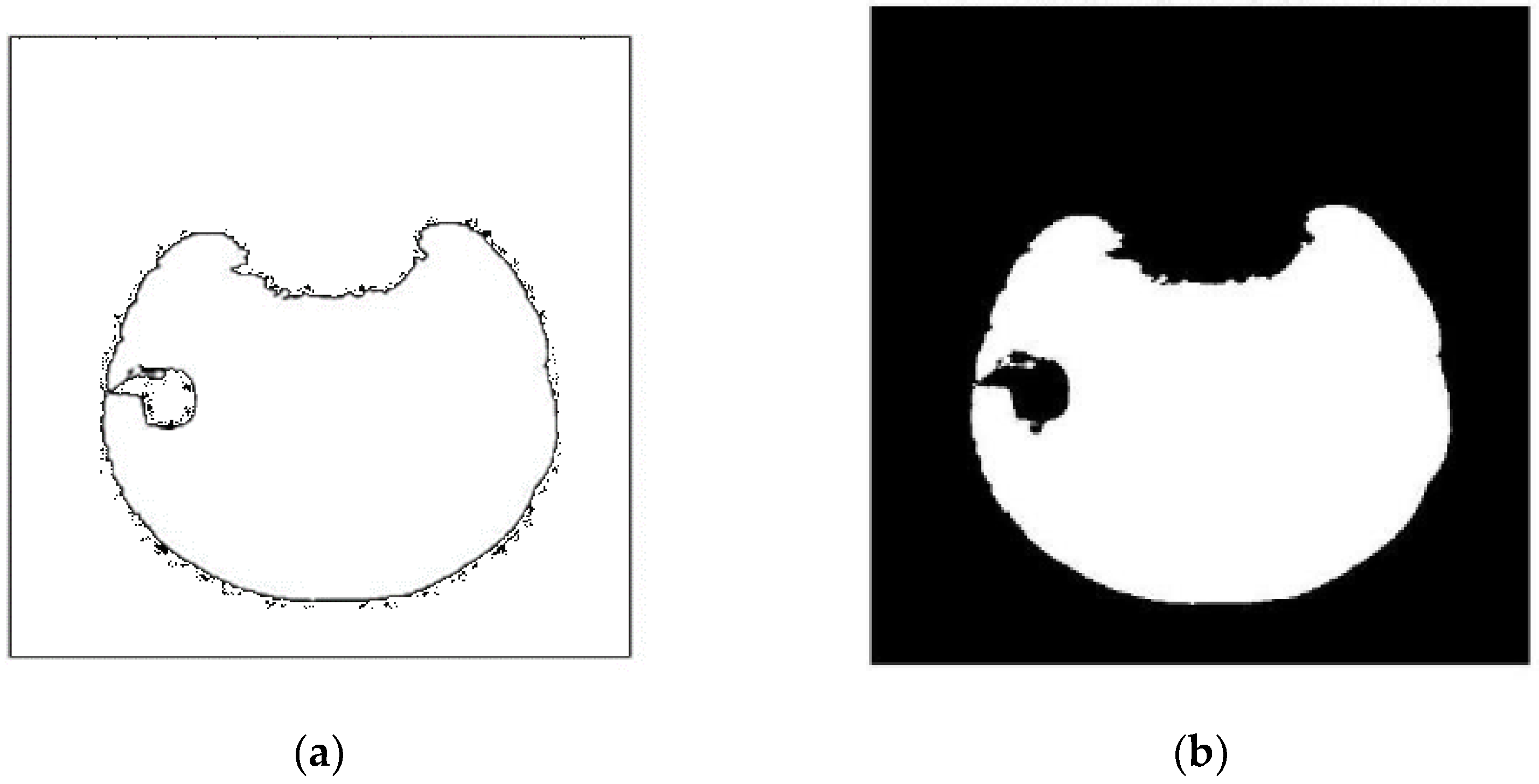
3.1. Dataset and Pre-Processing

This study utilizes magnetic resonance imaging (MRI) data from Medpol Hospital in Istanbul using GE HealthCare and Philips devices. The initial sample consisted of 253 individuals, each patient having a unique magnetic resonance (MR) image selected from a sequence of scans, typically from the T1, T2, or flair planes. After performing pre-processing on the images, including resizing them to 128 × 128 pixels, turning them to grayscale, and further pre-processing, a subset of these images is displayed in Figure 1. Then, 98 of these images were categorized with non-tumor classifications and 155 images were labeled with cancer.

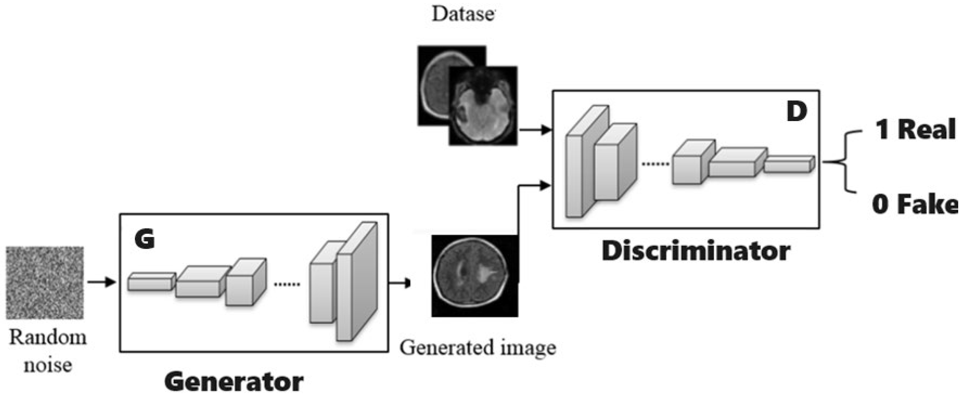
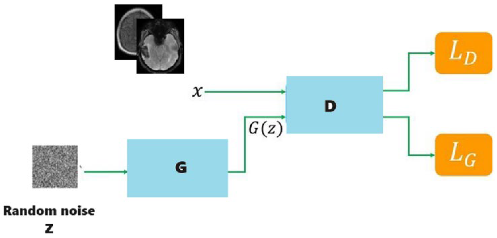
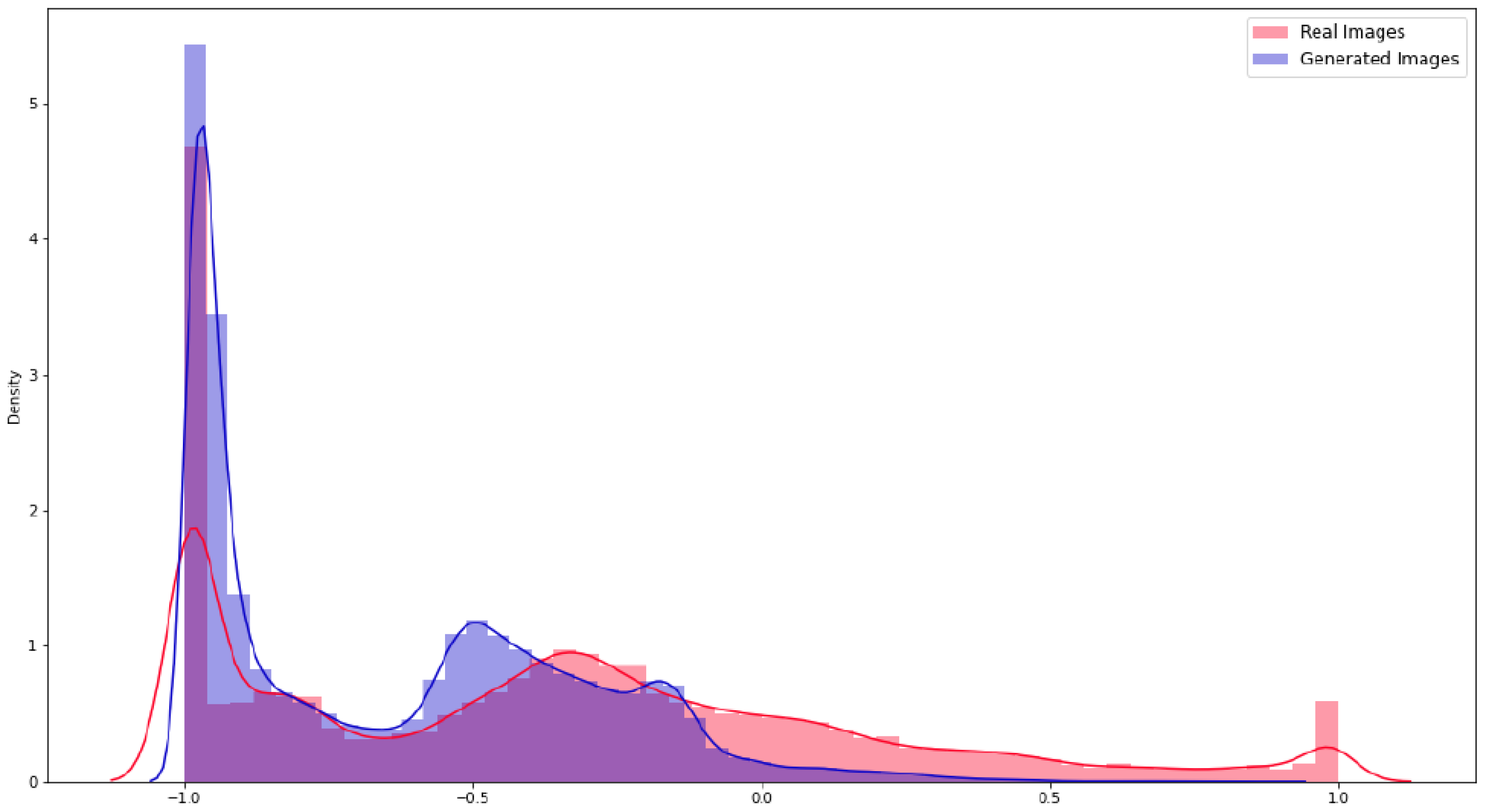
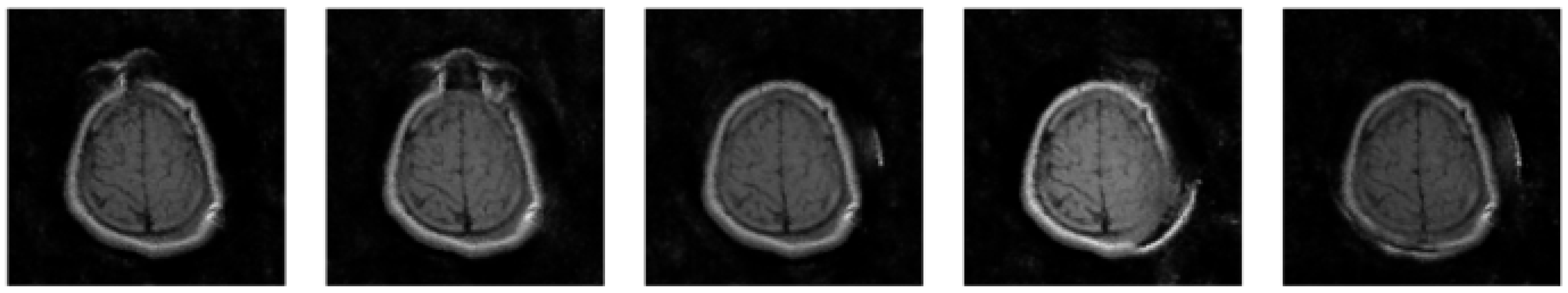
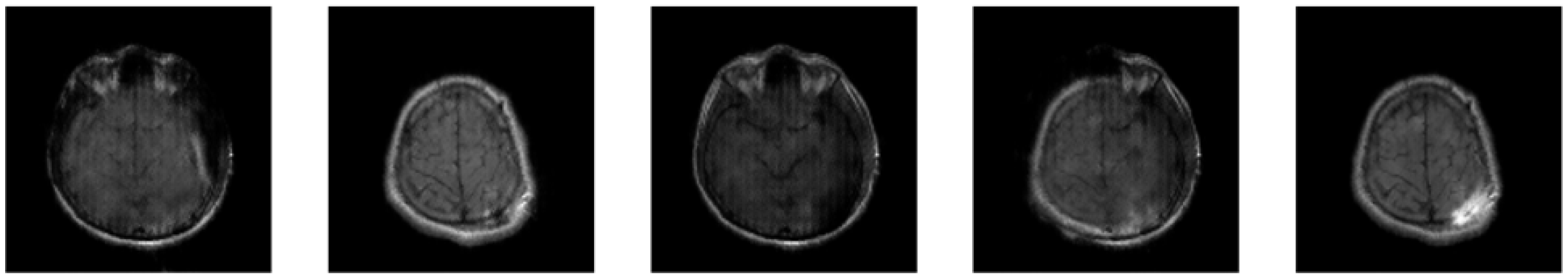
3.2. Data Augmentation and Generative Adversarial Networks

Machine learning algorithms used in the medical field face limitations in their use of medical data, mainly due to patient privacy concerns. In this context, traditional data augmentation methods are often used to collect more data for deep network training, a process which has many disadvantages, and many articles try to improve these methods in various research projects. Generative Adversarial Networks (GAN) to generate images for data augmentation can be used as one approach, which is considered purely computational and problem-solving. Deep generative models refer to a class of deep learning models that can learn the underlying data distribution from a given sample. These models can decrease data into its essential characteristics or generate novel data samples with diverse attributes. GANs are a type of implicit likelihood model that can create data samples by capturing the statistical distribution of the data. The GAN neural network was proposed in 2014 by Goodfellow and colleagues [22,23]. The GAN network comprises a Generator G(x) and a Discriminator D(x), both engaged in an adversarial game. Network D looks for any quality data coming from G to be fake. Any data from the real side re also labeled as accurate. Network G wants its generated data to safely pass through network D and to obtain the real data label. Both deep networks work simultaneously to learn and train the MRI data. Figure 2 shows the general structure of the GAN for MRI data generation.

In this system, the result ultimately depends on D’s decision, and the D network’s output is related to the loss functions. A GAN network has two cost functions: generator cost and discriminator cost. Both of these costs are defined based on the discriminator error. The overview is shown in Figure 3.

The loss function for discrimination evaluates the D network’s accuracy by examining the false and true prediction outcomes, as seen below. The number of errors in the D network determines the magnitude of loss. Finally, the error was rectified, and the parameters were revised. This function exhibits binomial loss. There are two terms used to refer to the input values in a system: “real input” for the value x and “fake input” for the value G(z). The initial component of the loss function for the actual input is denoted as Equation (1).

$$l_{{Discriminator}_1}=\log \delta \left(D\left(x\right)\right)$$

(1)

In the given relationship, σ represents a sigmoid excitation function that produces an output value ranging from 0 to 1. A value of 1 in the output indicates that the data is genuine, as determined by D. When the sigmoid output number approaches 1, the logarithm evaluates to 0. Therefore, we have no waste. Indeed, network D has accurately identified that input x corresponds to genuine data, and the second statement refers to the fabricated input (G(z)). We expect network D to classify these inputs as counterfeit and generate zero output for these specific input types in Equation (2).

$$l_{{Discriminator}_2}=\log \left(1-\delta \left(D\left(G\left(z\right)\right)\right)\right)$$

(2)

Now, we have to add the two expressions above together and write the discriminator loss function in Equation (3):

$$L_{Discriminator}=l_{{Discriminator}_1}+l_{{Discriminator}_2}=\log \delta \left(D\left(x\right)\right)+\log \left(1-\delta \left(D\left(G\left(z\right)\right)\right)\right)$$

(3)

The argument of logarithms is a value ranging from 0 to 1. For input values less than 1, the logarithm function yields a negative result. Therefore, the above phrase will consistently have a value lower than zero. Our objective is to optimize this correlation to achieve a zero value. Alternatively, similar to other neural networks, we introduce a negative (−sign to the relationship mentioned above to minimize the loss. Next, we need to optimize the above function using a negative value in Equation (4).

$$L_{Discriminator}=-\left(\log \delta \left(D\left(x\right)\right)+\log \left(1-\delta \left(D\left(G\left(z\right)\right)\right)\right)\right)$$

(4)

D’s ability to detect bogus or authentic G-generated data defines the generator loss function, as shown in the picture above. The D network informs the generator loss function that this data is entirely counterfeit. The dissipation function G is verified, and the dissipation value is computed. However, there is a crucial aspect to consider. Minimizing this expression implies that G can produce counterfeit data that closely resembles actual data, but D is deceived in its ability to identify counterfeit data. Network G desires the output to be directed to the numeral 1. It refers to the consumption of the actual data label. The generator loss function is defined as Equation (5):

$$l_{\mathrm{G}\mathrm{e}\mathrm{n}\mathrm{e}\mathrm{r}\mathrm{a}\mathrm{t}\mathrm{o}\mathrm{r}}=\log \delta \left(D\left(G\left(z\right)\right)\right)$$

(5)

Table 1. The internal structure and layers of the generative model.

Layer	Width	Hight	Depth	Stride	Layer Info
Dense	1	1	262,144	-	-
Activation	1	1	262,144	-	LeakyReLU
Reshape	32	32	256	-	-
ConVol-Transpose	64	64	256	2	-
Activation	64	64	256	-	LeakyReLU
ConVol-Transpose	128	128	256	2	-
Activation	128	128	256	-	LeakyReLU
ConVol	128	128	1	-	-
Activation	128	128	1	-	Tanh

and

Table 2. Internal structure and discriminating model layers.

Layer	Width	Hight	Depth	Stride	Layer Info
ConVol	128	128	64	-	-
Activation	128	128	64	-	LeakyReLU
ConVol	64	64	128	2	-
Activation	64	64	128	-	LeakyReLU
ConVol	32	32	128	2	-
Activation	32	32	128	-	LeakyReLU
ConVol	16	16	256	2	-
Activation	16	16	256	-	LeakyReLU
Flatten	1	1	65,536	-	-
Dropout	1	1	65,536	-	Rate 0.4
Dense	1	1	65,537	-	-
Activation	1	1	65,537	-	Sigmoid

show the combination of layers, the shape of each layer in pixels, and the parameters of the generator and separator network, respectively.

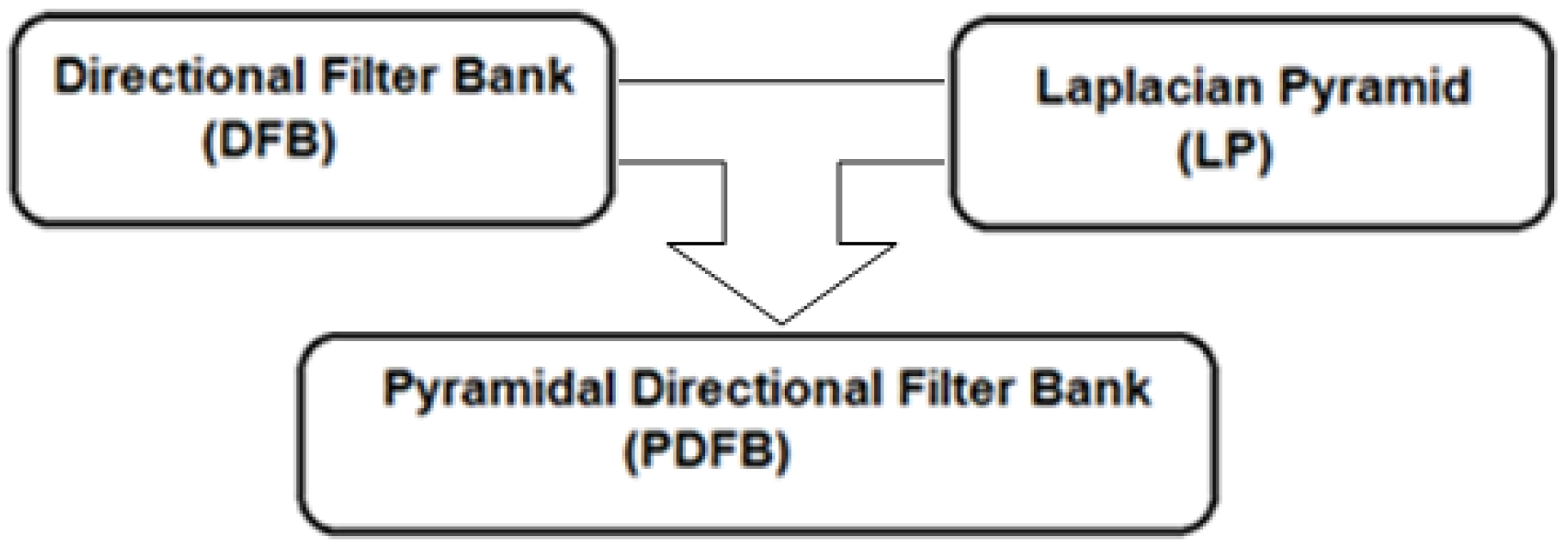
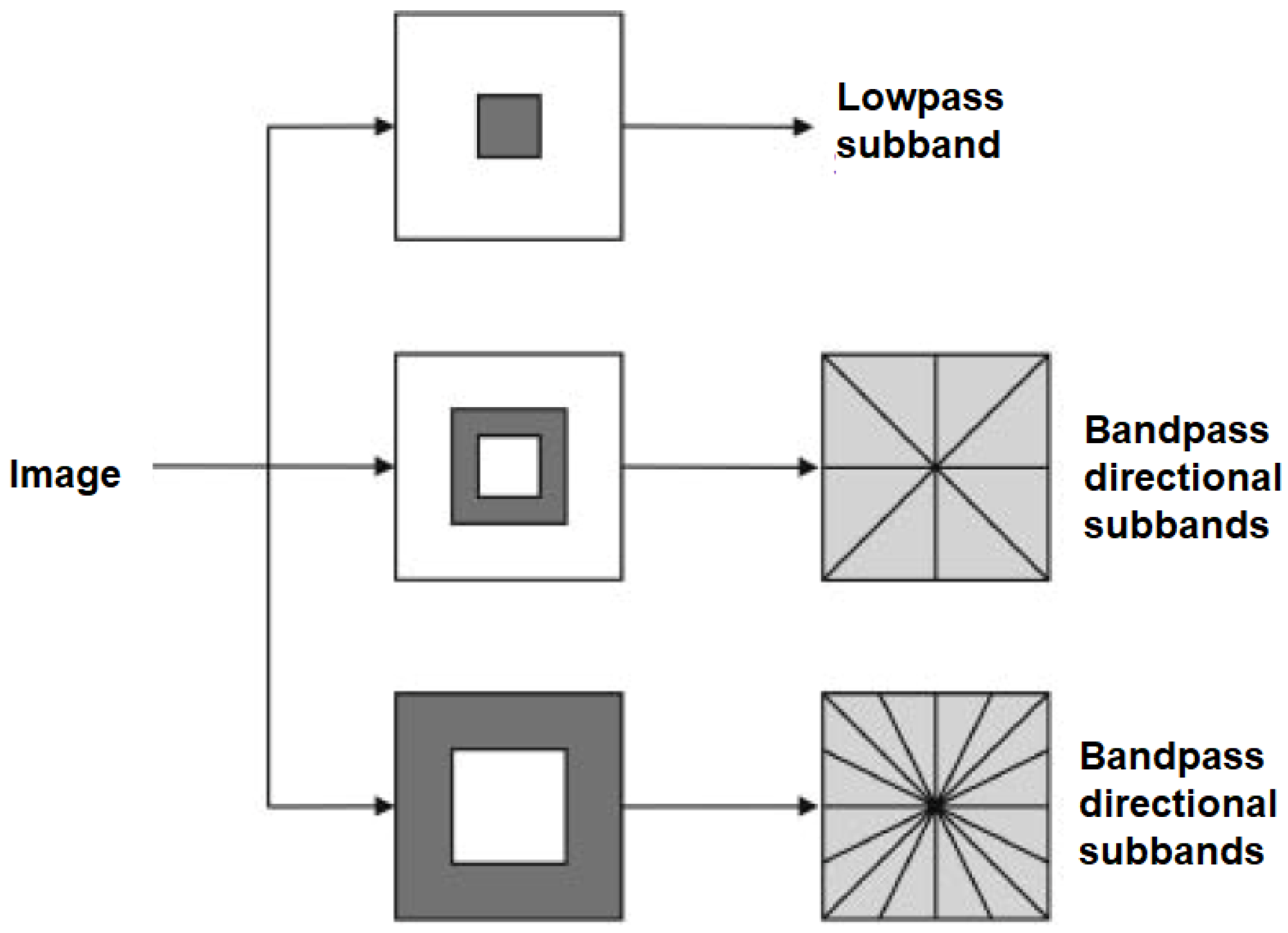
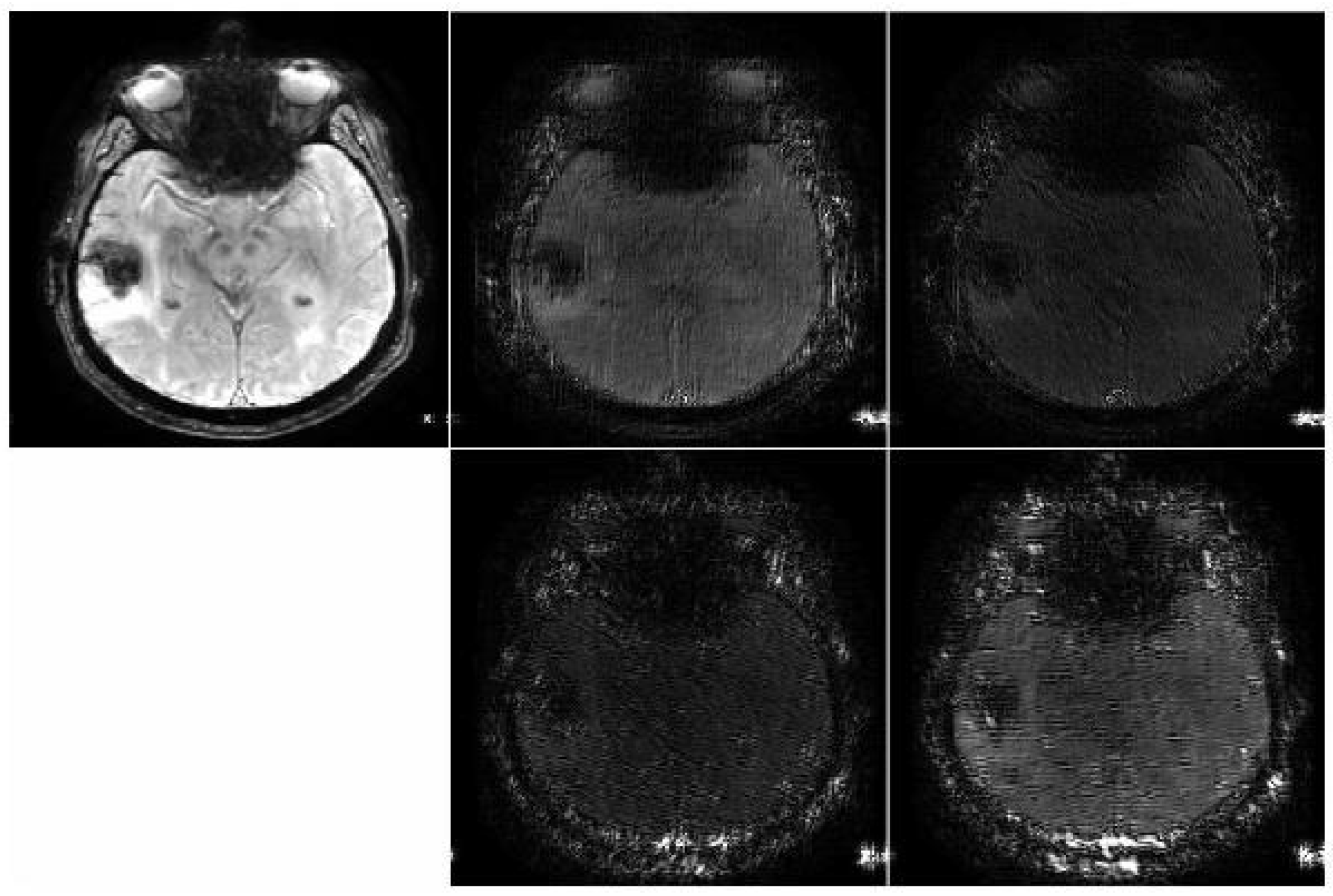
3.3. Data Processing and Contourlet Transform

Image segmentation is a task in computer analysis that falls under supervised learning. Supervised learning is a machine learning technique that entails utilizing datasets that have been annotated with labels. The model can gradually assess its accuracy and acquire knowledge using labeled inputs and outputs. Ground truth is utilized in the process of image segmentation. Ground truth is the process of training or validating a model using a dataset that has been labeled or tagged. Establishing the ground truth for datasets involves labor-intensive methods such as developing models, labeling data, and designing classifiers. A team of human annotators predominantly annotates the dataset’s ground truth labels. Subsequently, different methodologies are employed to compare and decide the target labels. More significant annotated datasets provide accurate reference points for machine learning and deep learning algorithms to enhance their pattern recognition abilities by including diverse data. Typically, labeling in image segmentation is laborious and requires manual effort from individuals using various software tools.

Do and Vetterli introduced contourlet transformation to improve image presentation by wavelet transform [24]. Later expanded by the same authors in [25], Contourlet transformation has been used in many fields, such as noise reduction [26,27], image feature extraction, image compression [28], face recognition [29], and image fusion [30] and edge detection [31]. The weaknesses of wavelet transformation have provoked the emergence of contourlet transformation. The wavelet exclusively handles one-dimensional units [32]. Furthermore, it is an exceptionally appropriate instrument for analyzing one-dimensional continuous signals. However, when dealing with 2D signals, such as images, it is expected to use the multiplication of individual wavelets resulting from the external expansion of 1D wavelets, and this approach is not suitable for accurately representing certain regions, especially those along image boundaries. Visual information relies heavily on the inherent geometric structures present in natural images.

The contourlet transform utilizes two filter banks from the Laplace pyramid plus a Directional Filter Bank (DFB), as depicted in Figure 4. The Laplace pyramid enables the detection of numerous boundaries and captures the discontinuities defined by the Laplace filter. The proportions of the image are halved at each level in the pyramid.

To provide a more comprehensive clarification, we will examine Figure 5. The bandpass is retrieved from the original image; in other words, this process is performed. Initially, the image’s high frequencies are computed. Next, the image undergoes a subtraction process to remove the lower frequencies. The intermediate frequencies are isolated, and directional operators are subsequently applied. When comparing the wavelet transform to the desired number of directions, we observe the extraction of several directions instead of just three. Each of these instructions assists us in identifying distinct boundaries of the image.

Similarly, the method is replicated in the low-frequency region using sample reduction. The intermediate frequencies are extracted using the DFB operator, and the procedure is repeated as often as required. Contourlet transformation involves utilizing the Laplacian pyramid with varying sizes and the DFB filter in different orientations.

Our goal in this transformation was to classify and label the pixels of the brain MRI image into two categories. In this way, the ground truth is obtained for each MR image using image processing techniques and contourlet transformation. We can apply the contourlet transformation in our MRI to find the boundaries and edges of the image in different levels and directions. Due to the two-dimensionality of the images, we performed the contourlet transformation in the second level in the four main directions, and the resulting images from this decomposition level are shown in Figure 6. To find the borders of the MR image, for simplicity and to obtain the desired results, we limited ourselves to analysis at two levels and the finding of the borders in four directions. Moreover, if the images are more complex or three-dimensional, we can carry out this conversion at the third level by analyzing them in eight directions.

Combining the original image’s decomposition coefficients in four directions was performed to find the image’s borders. After multiplying the coefficients of these four directions, the edges of the original image were obtained. By setting the binary threshold limit, we obtained the desired edges of the image and, finally, the mask that results from the ground truth is shown in Figure 7.

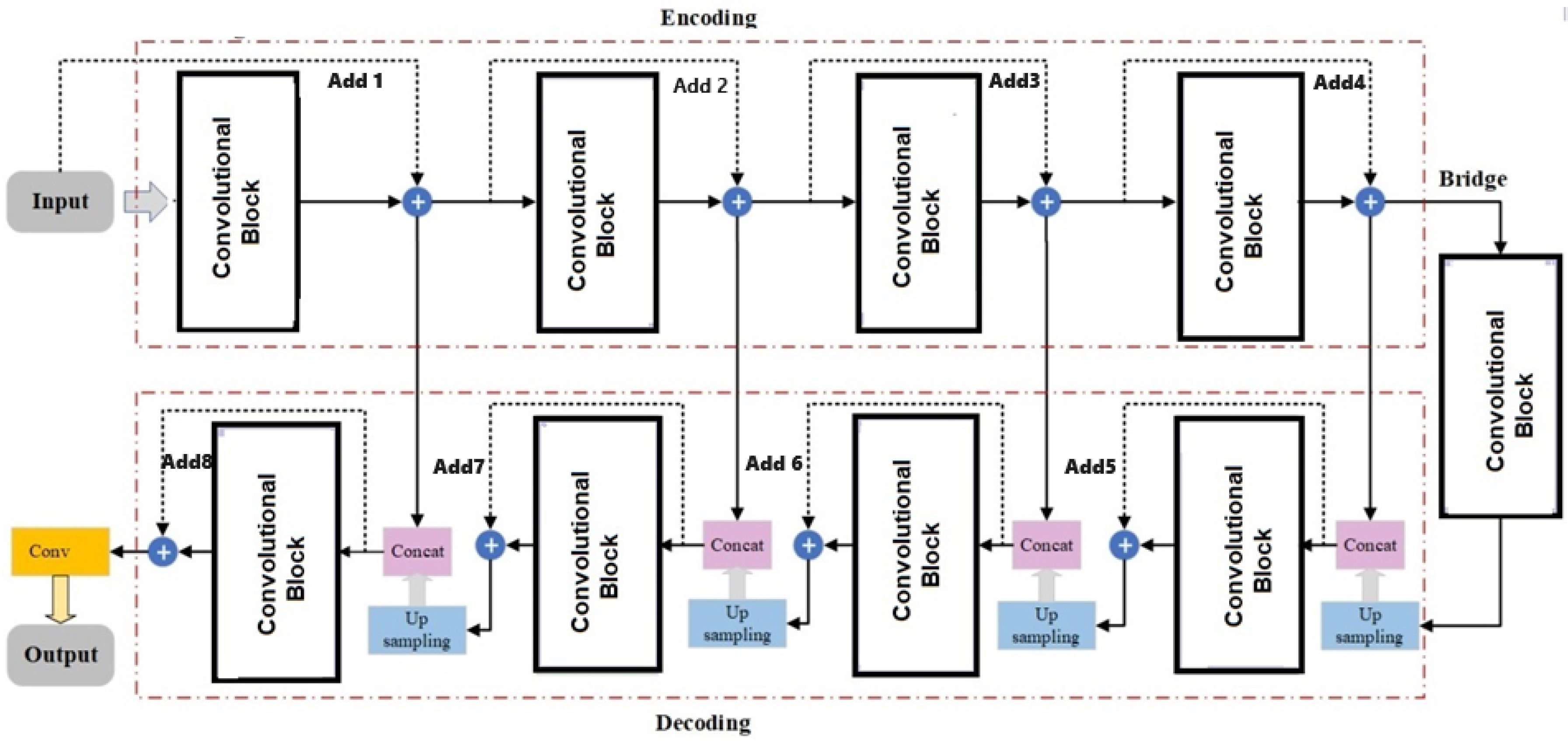
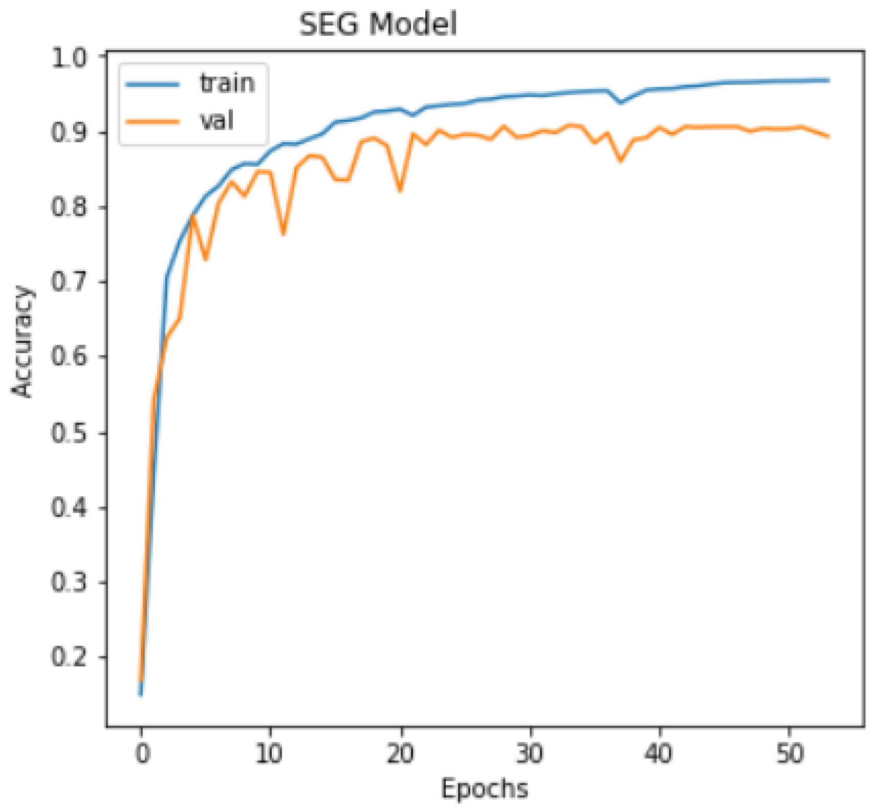
3.4. Segmentation Network

The U-Net technique has become increasingly popular in deep learning due to its accurate results, rapid processing speed, and minimal need for advanced and costly hardware [33,34]. The U-Net architecture is a convolutional neural network initially designed to segment semantic information in biological images. The network’s architectural design is strikingly similar to the contour of the English letter U, thereby earning it the famous moniker U-Net. The U-Net architecture has gained prominence in image segmentation due to its capacity to extract local and global properties by employing methods that can handle diverse scales. The U-Net design consists of three stages: encoder (contraction), bridge (bottleneck), and decoder (expansion). The encoder module leverages the attributes of the input image to reconstruct the segmented output. The decoder component arranges each pixel to display the segmented composition.

Augmenting the depth of a multi-layer neural network can amplify its efficacy. However, this could hinder the training process, decreasing the gradient [35]. Residual networks are formed by combining cumulative residual units [36] that aid the network’s training. Using jumpers within a residual unit allows the transmission of information beyond the unit’s boundaries. The primary function of the remaining blocks is to ease the transmission of information between layers, allowing for the creation of a more complex neural network. Utilizing channels decreases the computational expense and increases the dependence on those channels.

Our proposed model is an enhanced version that integrates U-Net and Residual networks, resulting in a higher learning capability. Figure 8 provides a concise summary of the intended architectural concept. Each convolutional block in the proposed framework is constructed from group normalization, leaky ReLU activation, and convolutional layers.

Table 3. The internal structure of the proposed blocks.

Layer	Encoder Block Structure	Decoder Block Structure
1	Add	Add
2	Activation	Activation
3	Max pooling	Up-sampling
4	ConVol	Concatenate
5	Batch Normalization	ConVol
6	Activation	Batch Normalization
7	ConVol	Activation
8	Batch Normalization	ConVol
9	ConVol	Batch Normalization
10	Batch Normalization	ConVol
11		Batch Normalization

shows the parameters and internal structure of the blocks.

4. Results and Discussion

Ultimately, by employing 253 photos and harnessing the computational capabilities of a 16 GB NVIDIA Tesla P100 graphics card, we utilized a generative network that operates on a random normal distribution to produce a sample that closely resembles the original distribution. For this network, we employed 12 epochs and 2000 steps for each epoch to generate images with a resolution of 128 by 128 pixels. The optimization algorithm we used was Adam, which had a learning rate of 0.0002.

Table 4. The results of the value of the loss functions.

EPOCH	Generator Loss	Discriminator Loss
1	2.7882	0.2121
2	1.7463	1.5576
3	1.4884	0.7854
4	2.0414	0.0719
5	2.1013	0.2531
6	4.2882	0.0856
7	6.8006	0.0007
8	4.5135	0.0913
9	2.9847	0.1567
10	7.7373	0.0208
11	3.3118	0.0454
12	2.7657	0.0614

displays the losses of the generating and discriminating functions at each stage.

By graphing the distribution of the generated images in the network and comparing it to the distribution of real images in Figure 9, we can observe the overlap between these two graphs. This overlap indicates that the generated samples closely resemble the real images. For a better understanding, sample images of the initial stage and stage 12 of the network are shown in Figure 10 and Figure 11, respectively.

Following the generation of new data and extraction of the mask for each image, it was time to assess the performance of the proposed deep neural network. Various evaluation criteria, such as accuracy, precision, sensitivity, and specificity, can be considered. Nevertheless, every measure possesses both benefits and drawbacks. Our strategy combines all of these aspects to attain exceptional outcomes.

The F1 Score is a metric that quantifies the balance between precision and recall. It is defined by Equation (6), which considers both accuracy and sensitivity. Equation (7) demonstrates the Dice criterion (DSC), which is frequently used as a criterion in segmentation problems. The DSC criterion is frequently used to calculate the similarity between two pictures. The Dice coefficient measures the level of similarity between the segmentation model’s outputs and the texture mask in image segmentation. Furthermore, with the Dice criterion, we utilize the Intersection-Over-Union (IoU) metric, also known as the Jaccard index. Equation (8) specifies the measure as the ratio of the overlapping area between the expected segmentation and the actual segmentation to the total area of the predicted segmentation and the actual segmentation.

$$F1 score=\frac{2\times (\mathrm{p}\mathrm{r}\mathrm{e}\mathrm{c}\mathrm{i}\mathrm{s}\mathrm{i}\mathrm{o}\mathrm{n}\times \mathrm{s}\mathrm{e}\mathrm{n}\mathrm{s}\mathrm{i}\mathrm{t}\mathrm{i}\mathrm{v}\mathrm{i}\mathrm{t}\mathrm{y})}{\mathrm{p}\mathrm{r}\mathrm{e}\mathrm{c}\mathrm{i}\mathrm{s}\mathrm{i}\mathrm{o}\mathrm{n}+\mathrm{s}\mathrm{e}\mathrm{n}\mathrm{s}\mathrm{i}\mathrm{t}\mathrm{i}\mathrm{v}\mathrm{i}\mathrm{t}\mathrm{y}}=\frac{2TP}{2\mathrm{T}\mathrm{P}+\mathrm{F}\mathrm{P}+\mathrm{F}\mathrm{N}}$$

(6)

The confusion matrix assigns TP to true positives, FP to false positives, and FN to false negatives.

$$DSC=\frac{2\left|X\cap Y\right|}{\left|X\right|+\left|Y\right|}$$

(7)

X is the mask of each image, and Y is the mask predicted in the image by our model.

$$IoU=\frac{\left|X\cap Y\right|}{\left|X\cup Y\right|}$$

(8)

The segmentation network employed in our study utilized the Dice Similarity Coefficient (DSC) loss function and the Adam optimizer to segment MR images automatically. Furthermore, the data in this network undergoes group normalization to enhance the network’s speed and stability. We had a grand total of 253 unique photos. The adversarial generating network generated ten additional images for each input image. Consequently, we possess a total of 2530 MR pictures, of which 80% (2024 images) were utilized for training, while 15% were allocated for validation. The dataset consisted of 379 photos, with the remaining 5% (127 images) reserved for testing the segmentation of deep neural networks. Figure 12 illustrates the proposed model’s training and validation dice scores for 60 epochs. The orange line in each figure corresponds to the validation data, while the blue line represents the test data. The graph illustrates consistent maintenance of high dice scores during the training period. After completing 50 epochs, it was seen that there was no significant alteration in the die score, leading to the decision to stop the training.

The primary objective of a deep neural network is to assess the model’s performance and identify the components that require optimization. The determination is often achieved by comparing the accuracy metrics of the test data with the validation data to assess the network’s suitability. If a substantial disparity exists between the two, it can be deduced that our network is displaying signs of overfitting and overtraining. Furthermore, “underfit mode” describes a model that cannot accurately represent the training data, resulting in substantial mistakes. The validation data should ideally exhibit accuracy levels comparable to or slightly lower than the accuracy seen in the test data. Figure 13 displays the training and validation losses of the model. The proposed method provides a substantial decrease in redundancies during the training of neural networks, distinguishing it from earlier networks. Augmenting the number of iterations in the training of deep neural networks is well acknowledged to lead to an increased requirement for computational resources.

The assessment standards for all segmented MRI images utilizing the proposed model in two modes, employing the GAN network for data creation and without it, are outlined in

Table 5. Performance results of segmentation network with a GAN network and without GAN on our dataset.

Evaluation Criteria	DSC	IoU	Precision	Specificity	Sensitivity
With GAN	0.9434	0.8928	0.9390	0.9390	0.9479
Without GAN	0.8070	0.6764	0.7863	0.7807	0.8288

. Furthermore, to assess the residual network’s performance more precisely, we compared the regular Unet network and the suggested residual network in

Table 6. Comparing the performance results of the proposed network with the standard Unet network in our brain MRI dataset.

Criteria	DSC	IoU
Our segmentation model	0.9434	0.8928
Standard U net	0.9281	0.8658

. The image segmentation result for a sample is displayed in Figure 14.

5. Discussion and Conclusions

This study employed an automated method for segmenting brain tumors in brain MRI datasets. This was achieved by integrating a generative adversarial neural network system, which generates and enhances the data, with a deep neural network for image segmentation training. The contourlet transform connected these two networks and effectively retrieved the accurate ground truth for each brain MRI. The distribution graph of the generated data, which exhibits a significant degree of overlap with the distribution of the original data, demonstrated the efficacy of the adversarial generator network in producing fresh data of superior quality. In the contourlet transformation stage, the background truth of each image was effectively retrieved due to its strong capability in border recognition. It is feasible, and we can employ this conversion to extract masks from 3D images. The segmentation deep neural network demonstrated superior performance during training and a faster convergence rate than traditional topologies, enhancing the integration of residual learning models. Residual blocks effectively transmitted local properties within the segmentation system to the entire system, making them well-suited for automated resolution of combinatorial segmentation issues. By integrating supervised learning with unsupervised learning, this system can be used for various datasets, even those with limited samples, and offers a completely automated approach to image segmentation. The proposed approach was evaluated using the dataset from Medipol Hospital in Istanbul. The test results demonstrated the significant efficacy of the suggested technique, as seen by the dice scores of 0.9434.

References

1. Abd-Ellah, M.K.; Awad, A.I.; Khalaf, A.A.; Hamed, H.F. A review on brain tumor diagnosis from MRI images: Practical implications, key achievements, and lessons learned. Magn. Reson. Imaging 2019, 61, 300–318. [Google Scholar] [CrossRef]
2. Wadhwa, A.; Bhardwaj, A.; Verma, V.S. A review on brain tumor segmentation of MRI images. Magn. Reson. Imaging 2019, 61, 247–259. [Google Scholar] [CrossRef] [PubMed]
3. Zhao, X.; Wu, Y.; Song, G.; Li, Z.; Zhang, Y.; Fan, Y. A deep learning model integrating FCNNs and CRFs for brain tumor segmentation. Med. Image Anal. 2018, 43, 98–111. [Google Scholar] [CrossRef] [PubMed]
4. Ilunga–Mbuyamba, E.; Avina–Cervantes, J.G.; Cepeda–Negrete, J.; Ibarra–Manzano, M.A.; Chalopin, C. Automatic selection of localized region-based active contour models using image content analysis applied to brain tumor segmentation. Comput. Biol. Med. 2017, 91, 69–79. [Google Scholar] [CrossRef] [PubMed]
5. Iqbal, S.; Ghani, M.U.; Saba, T.; Rehman, A. Brain tumor segmentation in multi-spectral MRI using convolutional neural networks (CNN). Microsc. Res. Tech. 2018, 81, 419–427. [Google Scholar] [CrossRef] [PubMed]
6. Ker, J.; Wang, L.; Rao, J.; Lim, T. Deep Learning Applications in Medical Image Analysis. IEEE Access 2017, 6, 9375–9389. [Google Scholar] [CrossRef]
7. Saman, S.; Narayanan, S.J. Survey on brain tumor segmentation and feature extraction of MR images. Int. J. Multimedia Inf. Retr. 2019, 8, 79–99. [Google Scholar] [CrossRef]
8. Pereira, S.; Pinto, A.; Alves, V.; Silva, C.A. Brain tumor segmentation using convolutional neural networks in MRI images. IEEE Trans. Med. Imaging 2016, 35, 1240–1251. [Google Scholar] [CrossRef]
9. More, S.S.; Mange, M.A.; Sankhe, M.S.; Sahu, S.S. Convolutional neural network based brain tumor detection. In Proceedings of the 2021 5th International Conference on Intelligent Computing and Control Systems (ICICCS), Madurai, India, 6–8 May 2021; pp. 1532–1538. [Google Scholar]
10. Spinner, T.; Schlegel, U.; Schafer, H.; El-Assady, M. explAIner: A visual analytics framework for interactive and explainable machine learning. IEEE Trans. Vis. Comput. Graph. 2019, 26, 1064–1074. [Google Scholar] [CrossRef]
11. Piccialli, F.; Di Somma, V.; Giampaolo, F.; Cuomo, S.; Fortino, G. A survey on deep learning in medicine: Why, how and when? Inf. Fusion 2021, 66, 111–137. [Google Scholar] [CrossRef]
12. Ben Naceur, M.; Saouli, R.; Akil, M.; Kachouri, R. Fully automatic brain tumor segmentation using end-to-end incremental deep neural networks in MRI images. Comput. Methods Programs Biomed. 2018, 166, 39–49. [Google Scholar] [CrossRef] [PubMed]
13. Raza, R.; Bajwa, U.I.; Mehmood, Y.; Anwar, M.W.; Jamal, M.H. dResU-Net: 3D deep residual U-Net based brain tumor segmentation from multimodal MRI. Biomed. Signal Process. Control 2023, 79, 103861. [Google Scholar] [CrossRef]
14. Gull, S.; Akbar, S.; Shoukat, I.A. A Deep Transfer learning approach for automated detection of brain tumor through magnetic resonance imaging. In Proceedings of the 2021 International Conference on Innovative Computing (ICIC), Online, 15–16 September 2021; pp. 1–6. [Google Scholar]
15. Karayegen, G.; Aksahin, M.F. Brain tumor prediction on MR images with semantic segmentation by using deep learning network and 3D imaging of tumor region. Biomed. Signal Process. Control 2021, 66, 102458. [Google Scholar] [CrossRef]
16. Akbar, A.S.; Fatichah, C.; Suciati, N. Single level UNet3D with multipath residual attention block for brain tumor segmentation. J. King Saud Univ. Comput. Inf. Sci. 2022, 34, 3247–3258. [Google Scholar] [CrossRef]
17. Ullah, Z.; Usman, M.; Jeon, M.; Gwak, J. Cascade multiscale residual attention CNNs with adaptive ROI for automatic brain tumor segmentation. Inf. Sci. 2022, 608, 1541–1556. [Google Scholar] [CrossRef]
18. Zhou, X.; Li, X.; Hu, K.; Zhang, Y.; Chen, Z.; Gao, X. ERV-Net: An efficient 3D residual neural network for brain tumor segmentation. Expert Syst. Appl. 2021, 170, 114566. [Google Scholar] [CrossRef]
19. Talo, M.; Baloglu, U.B.; Yıldırım, Ö.; Acharya, U.R. Application of deep transfer learning for automated brain abnormality classification using MR images. Cogn. Syst. Res. 2019, 54, 176–188. [Google Scholar] [CrossRef]
20. Chawla, R.; Beram, S.M.; Murthy, C.R.; Thiruvenkadam, T.; Bhavani, N.; Saravanakumar, R.; Sathishkumar, P. Brain tumor recognition using an integrated bat algorithm with a convolutional neural network approach. Meas. Sensors 2022, 24, 100426. [Google Scholar] [CrossRef]
21. Ghassemi, N.; Shoeibi, A.; Rouhani, M. Deep neural network with generative adversarial networks pre-training for brain tumor classification based on MR images. Biomed. Signal Process. Control 2020, 57, 101678. [Google Scholar] [CrossRef]
22. Goodfellow, I.; Pouget-Abadie, J.; Mirza, M.; Xu, B.; Warde-Farley, D.; Ozair, S.; Courville, A.; Bengio, Y. Generative adversarial networks. Commun. ACM 2020, 63, 139–144. [Google Scholar] [CrossRef]
23. Salimans, T.; Goodfellow, I.; Zaremba, W.; Cheung, V.; Radford, A.; Chen, X. Improved techniques for training gans. Adv. Neural Inf. Process. Syst. 2016, 2234–2242. [Google Scholar]
24. Do, M.N.; Vetterli, M. Contourlets: A directional multiresolution image representation. In Proceedings of the International Conference on Image Processing, New York, NY, USA, 22–25 September 2002. [Google Scholar]
25. Do, M.; Vetterli, M. The contourlet transform: An efficient directional multiresolution image representation. IEEE Trans. Image Process. 2005, 14, 2091–2106. [Google Scholar] [CrossRef] [PubMed]
26. Mejía Muñoz, J.M.; de Jesús Ochoa Domínguez, H.; Ortega Máynez, L.; Vergara Villegas, O.O.; Cruz Sánchez, V.G.; Gordillo Castillo, N.; Gutiérrez Casas, E.D. SAR image denoising using the non-subsampled contourlet transform and morphological operators. In Proceedings of the Advances in Artificial Intelligence, 9th Mexican International Conference on Artificial Intelligence, MICAI 2010, Pachuca, Mexico, 8–13 November 2010; Springer: Berlin/Heidelberg, Germany, 2010; pp. 337–347. [Google Scholar]
27. Sadreazami, H.; Ahmad, M.O.; Swamy, M. A study on image denoising in contourlet domain using the alpha-stable family of distributions. Signal Process. 2016, 128, 459–473. [Google Scholar] [CrossRef]
28. Bi, X.; Chen, X.; Li, X. Medical image compressed sensing based on contourlet. In Proceedings of the 2009 2nd International Congress on Image and Signal Processing, Tianjin, China, 17–19 October 2009; pp. 1–4. [Google Scholar]
29. Sajedi, H.; Jamzad, M. A contourlet-based face detection method in color images. In Proceedings of the 2007 Third International IEEE Conference on Signal-Image Technologies and Internet-Based System, Shanghai, China, 16–18 December 2007; pp. 727–732. [Google Scholar]
30. Khare, A.; Srivastava, R.; Singh, R. Edge preserving image fusion based on contourlet transform. In Proceedings of the International Conference on Image and Signal Processing, Agadir, Morocco, 28–30 June 2012; pp. 93–102. [Google Scholar]
31. Xia, L.; Fangfei, Y.; Ligang, S. Image Edge Detection Based on Contourlet Transform Combined with the Model of Anisotropic Receptive Fields. In Proceedings of the 2014 Fifth International Conference on Intelligent Systems Design and Engineering Applications, Hunan, China, 15–16 June 2014; pp. 533–536. [Google Scholar]
32. Fernandes, F.; van Spaendonck, R.; Burrus, C. A new framework for complex wavelet transforms. IEEE Trans. Signal Process. 2003, 51, 1825–1837. [Google Scholar] [CrossRef]
33. Çiçek, Ö.; Abdulkadir, A.; Lienkamp, S.S.; Brox, T.; Ronneberger, O. 3D U-Net: Learning dense volumetric segmentation from sparse annotation. In Proceedings of the Medical Image Computing and Computer-Assisted Intervention–MICCAI 2016: 19th International Conference, Athens, Greece, 17–21 October 2016; Springer: Berlin/Heidelberg, Germany, 2016; pp. 424–432. [Google Scholar]
34. Ronneberger, O.; Fischer, P.; Brox, T. U-net: Convolutional networks for biomedical image segmentation. In Proceedings of the Medical Image Computing and Computer-Assisted Intervention–MICCAI 2015: 18th International Conference, Munich, Germany, 5–9 October 2015; Springer: Berlin/Heidelberg, Germany, 2015; pp. 234–241. [Google Scholar]
35. He, K.; Zhang, X.; Ren, S.; Sun, J. Deep residual learning for image recognition. In Proceedings of the IEEE Conference on Computer Vision and Pattern Recognition, Las Vegas, NV, USA, 27–30 June 2016; pp. 770–778. [Google Scholar]
36. He, K.; Zhang, X.; Ren, S.; Sun, J. Identity mappings in deep residual networks. In Proceedings of the Computer Vision–ECCV 2016, Presented at the 14th European Conference, Amsterdam, The Netherlands, 11–14 October 2016; Springer: Berlin/Heidelberg, Germany, 2016; pp. 630–645. [Google Scholar]
Figure 1. Example of MR images after initial pre-processing.
Algorithms 17 00130 g001
Figure 2. The general structure of the GAN for MRI data generation.
Algorithms 17 00130 g002
Figure 3. Cost functions in the GAN network.
Algorithms 17 00130 g003
Figure 4. The structure of the filters that make up the contourlet transform.
Algorithms 17 00130 g004
Figure 5. The frequency structure of the contourlet transform.
Algorithms 17 00130 g005
Figure 6. Decomposition of the second level in four directions in sample MRI.
Algorithms 17 00130 g006
Figure 7. (a) The edges of the images; (b) ground truth related to the sample MRI.
Algorithms 17 00130 g007
Figure 8. The Proposed ResU-Net Architecture.
Algorithms 17 00130 g008
Figure 9. Distribution of the original dataset with network-constructed data.
Algorithms 17 00130 g009
Figure 10. The images are generated in the initial iteration of the GAN network.
Algorithms 17 00130 g010
Figure 11. Images produced in the last iteration of the GAN network.
Algorithms 17 00130 g011
Figure 12. Training and Validation accuracy in our model.
Algorithms 17 00130 g012
Figure 13. Training and Validation Loss in our Model.
Algorithms 17 00130 g013
Figure 14. Image segmentation result for a sample MRI. (a) Brain MR; (b) the original mask is made with contourlet transformation; (c) predicted mask by the segmentation network.
Algorithms 17 00130 g014