

Analysis of a Two-Step Gradient Method with Two Momentum Parameters for Strongly Convex Unconstrained Optimization

Abstract
:1. Introduction
2. Analysis of Two-Step Method
2.1. Convergence Conditions
- (1)
- Let the new variable be introduced. Then, method (6) can be rewritten as a single-step method:where matrix T is written asThis method converges if, and only if, (spectral radius of matrix T) is strictly less than unity [3].Matrix A can be represented by the spectral decomposition , where is the diagonal matrix of eigenvalues of A, S is a matrix of eigenvectors, and . The following transformation of T can be introduced: , whereMatrix has the same eigenvalues, as matrix T.Let us demonstrate that has the same spectrum as the following matrix:where are matrices, which are presented asMatrix is presented aswhere , , , . The determinant of this matrix is computed by the following rule [30]:where , .The determinant of the block-diagonal matrix is written asand, as can be seen, it is equal to . So, both matrices have the same eigenvalues , and these eigenvalues are computed as eigenvalues of matrices .
- (2)
- According to the result presented above, the analysis of eigenvalues of T leads to the analysis of roots of an algebraic equation:In order to guarantee convergence, parameters should be chosen in a way which guarantees that . For obtaining these conditions, we perform conformal mapping of the interior of the unit circle to the set with use of the following function:The conditions on coefficients of (10) guarantee roots are provided by the Routh–Hurwitz criterion [30,31]. The Hurwitz matrix for (10) is written asThe conditions of the Routh–Hurwitz criterion lead to two inequalities:Inequity (11) is valid , according to the ranges of values of stated in the conditions of the theorem. Inequity (12) is rewritten asand it is valid for values of h chosen from Inequity (7). This, condition (7) guarantees that , and as a consequence that under the stated conditions. This leads to the convergence of (6) for any .
2.2. Analysis of Convergence Rate
- (1)
- Let us obtain the expression for . For in the case of , the following inequality takes place: and if , and in this case . If , we obtain that and . So, if and , we have that .If and , we have that , and for we have that if , then . If , then and . So if and , we obtain that .For , it is easy to see that . The case of and case are trivial to analyze. Thus, it is demonstrated that
- (2)
- Let us analyze the behavior of for . The expression for D is written asSo, the non-negative values of D are associated with the solutions of the following inequality:The corresponding discriminant is equal to . As can be seen, solutions to this inequality exist, whenThe opposite inequality guarantees that it is valid for all . For analysis of the general situation of the sign of D this restriction is too strict, so we consider the case of condition (14).The case of leads to the investigation of function . Condition leads to the restriction , which is valid for . It should be noted that this condition correlates with (7) for values of , under condition . The derivative of is written asand for , it is strictly negative, so decreases on the considered interval and its maximum is equal to .For , we obtain that . The case corresponds to the interval , where r decreases, and case corresponds to , where r increases. So, the maximum of r in this situations is realized in point or .For , two situations should be considered. For , the behavior of function should be analyzed. Its derivative is written asand according to , we can see that if , will be negative, so decreases. Let us determine where this inequality is valid:soFunction is strictly positive, whenAs can be seen, this inequality is valid when condition (14) is realized on values of . So, in the interval , function decreases.Positive values of can be realized when the following inequality is valid:which leads to . According to , this leads to the evident inequality , which takes place for under condition (15).Let us demonstrate that (16) correlates with (14): Inequity (16) leads to , which leads to the following inequality:which is equivalent towhich is equivalent to (14).It is easy to see thatso, when (corresponds to ), r decreases when and increases when and its maximum is realized in the boundary point.The case leads to the analysis of function on the interval, defined by inequality (see case )The first derivative of is written asAccording to , we obtain that if (this takes place when ), this derivative is strictly positive. According to (17), it is valid for the interval defined by (18), so and, as a consequence, function r increases in the case of corresponding to (18) and its maximum takes place in the right boundary point , if intervals and (18) have an intersection.Thus, for all values of D, we can see that r reaches its maximum value at the boundaries of interval .
2.3. Optimal Parameters
- (1)
- (2)
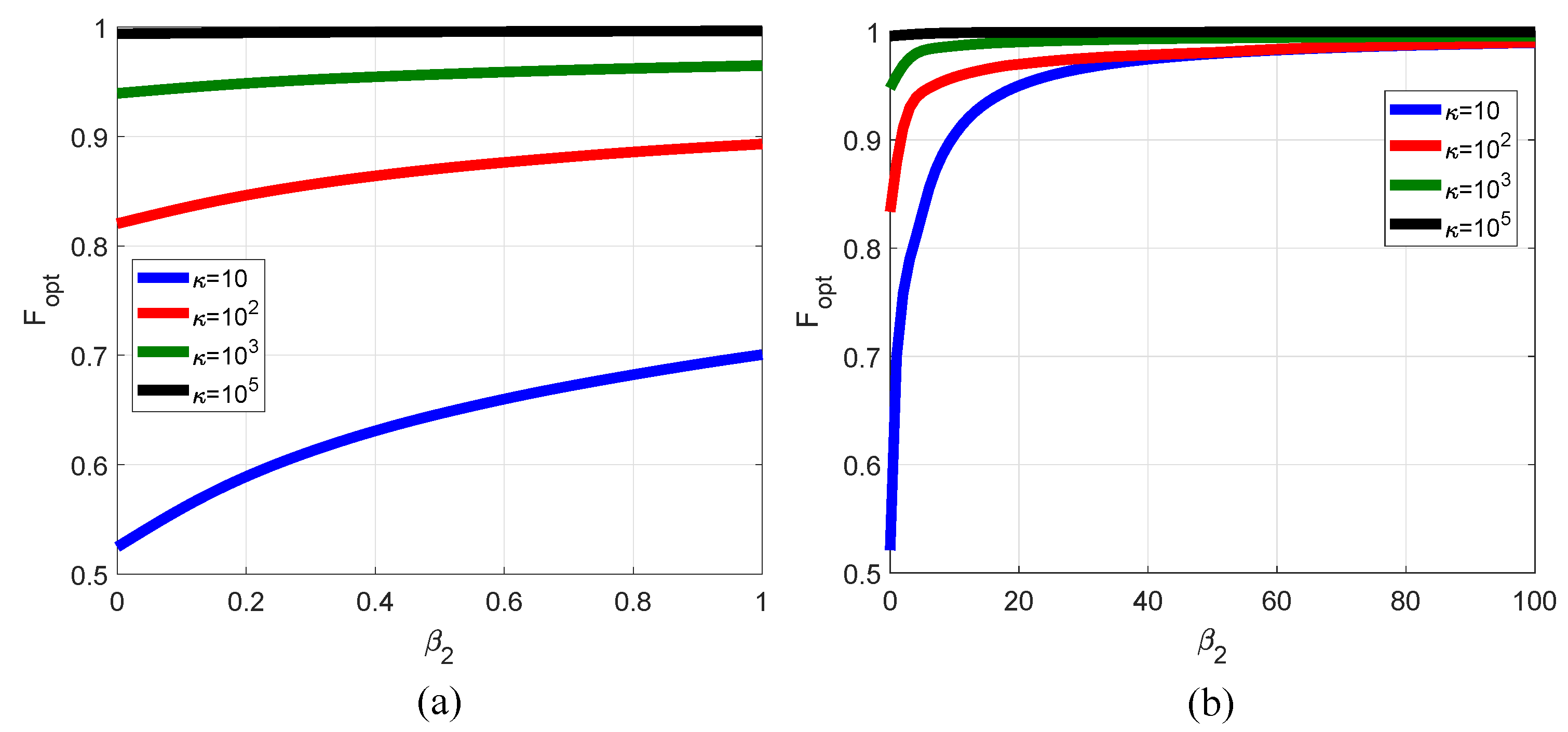
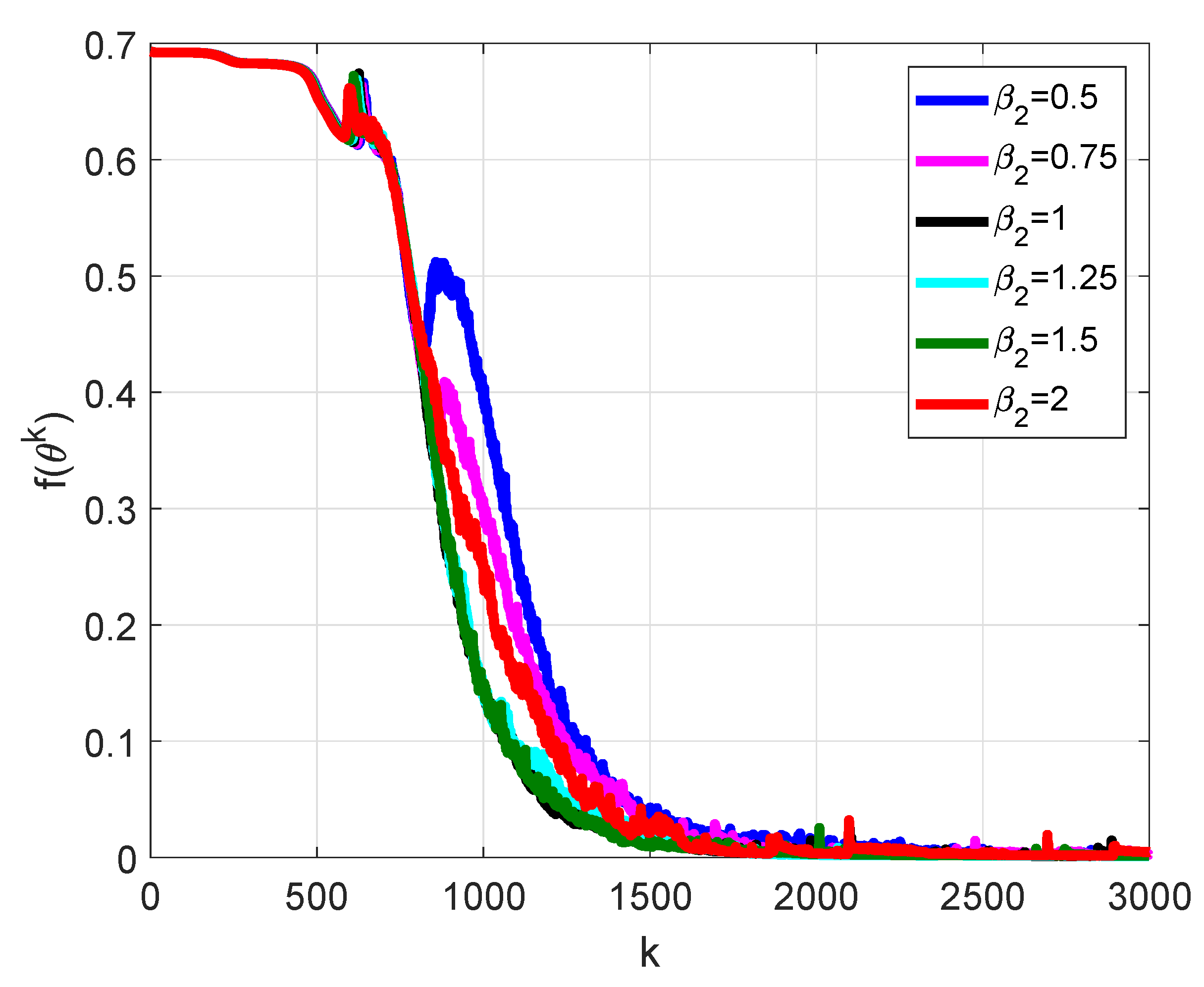
- Nesterov’s accelerated gradient method for a strongly convex quadratic function (Nesterov2) [28]:The numerical solution to problem (19) is realized using the same method as for problem (21), but for the Nelder–Mead method, four ’good’ points are obtained with a random search. The interval on is bounded by 0.5, according to the behavior, illustrated in Figure 1.
2.4. Equivalent ODE
3. Numerical Experiments and Discussion
3.1. Rosenbrock Function
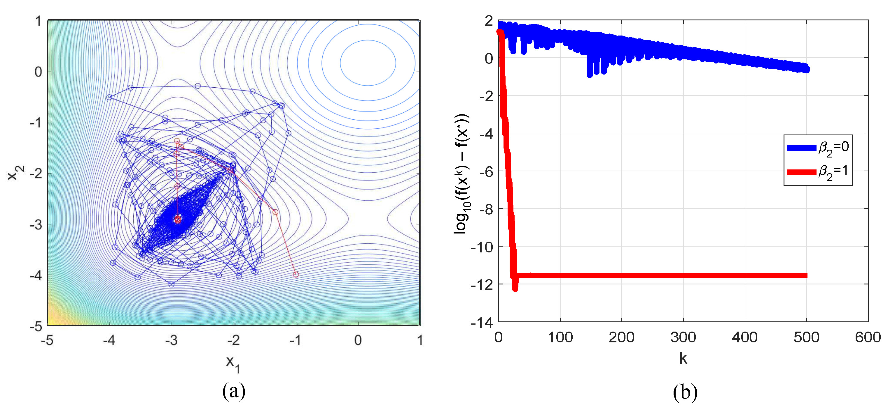
3.2. Himmelblau Function
3.3. Styblinski–Tang Function
3.4. Zakharov Function
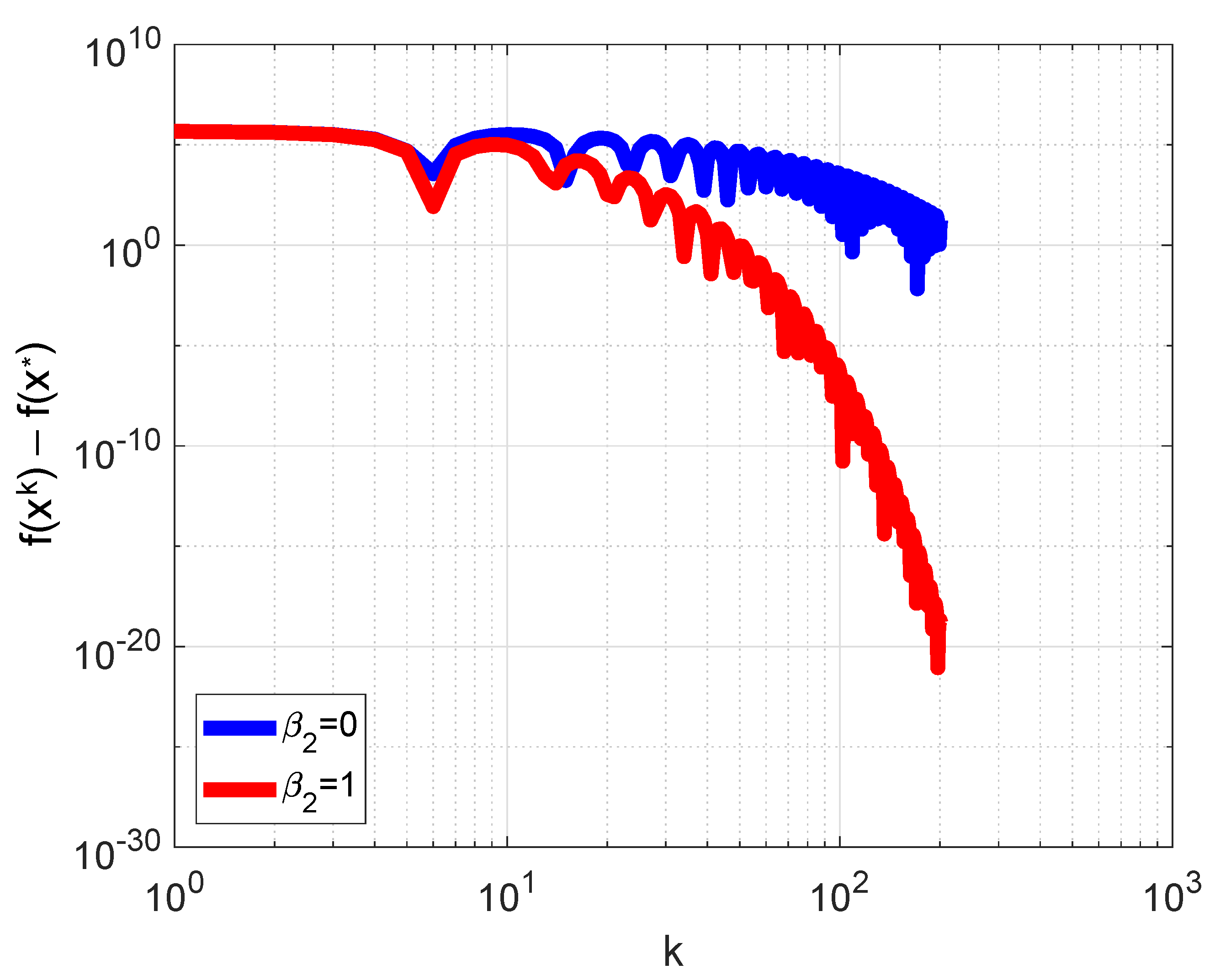
3.5. Non-Convex Function in Multidimensional Space
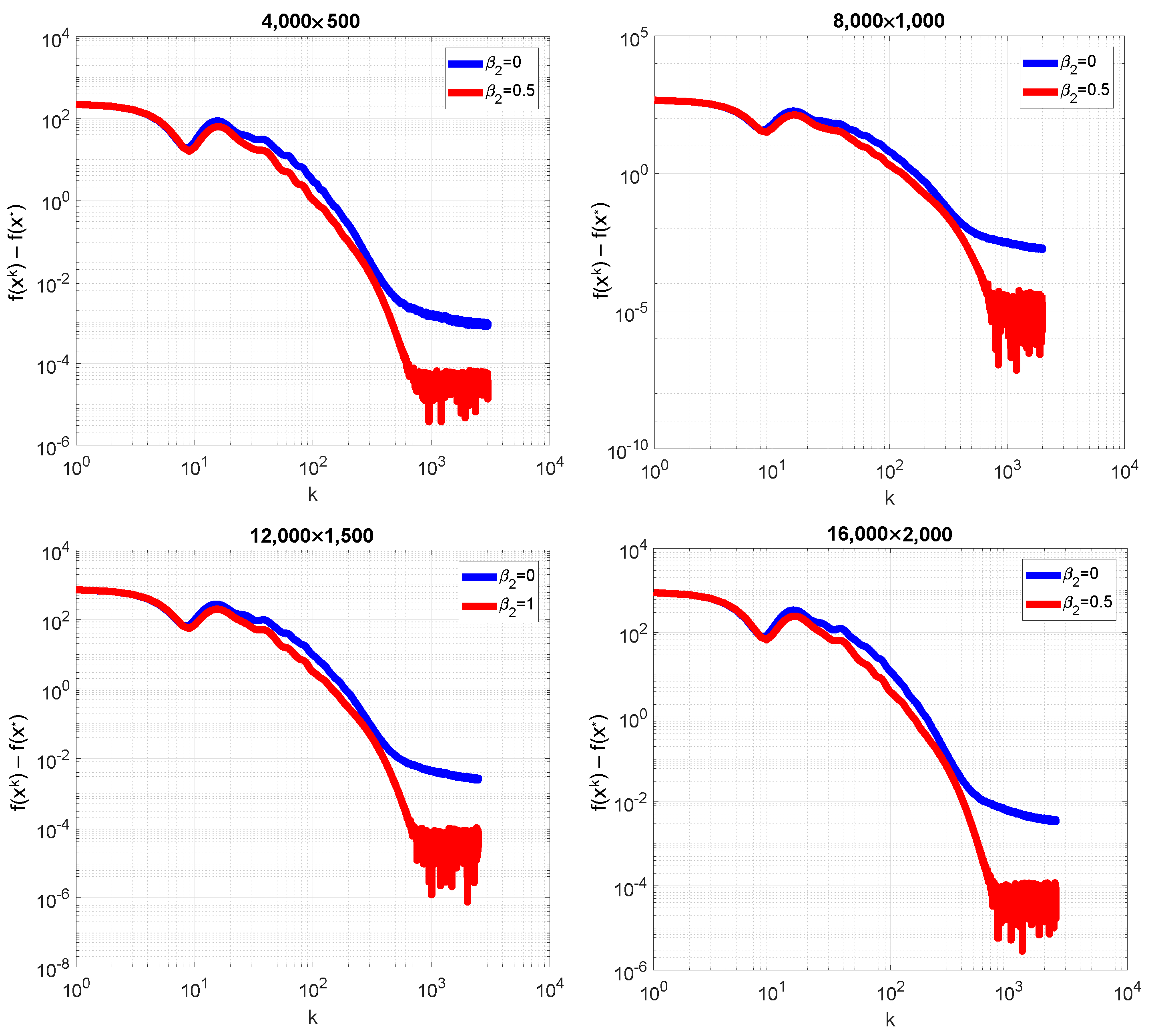
3.6. Smoothed Elastic Net Regularization
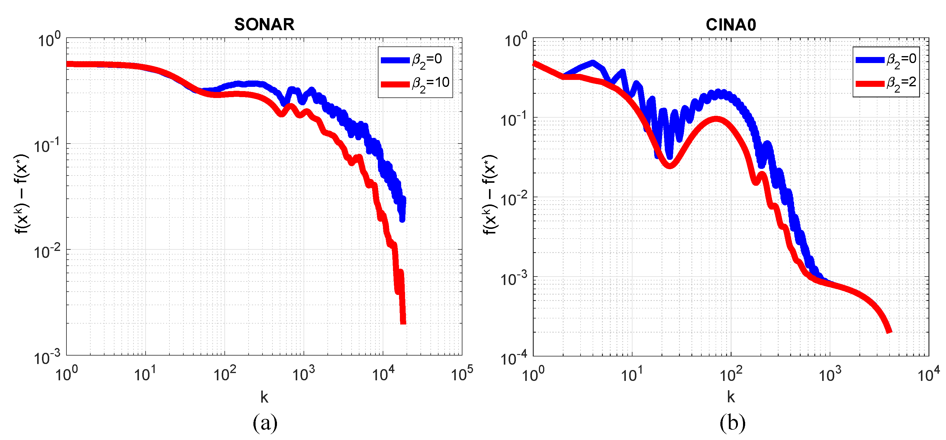
3.7. Logistic Regression
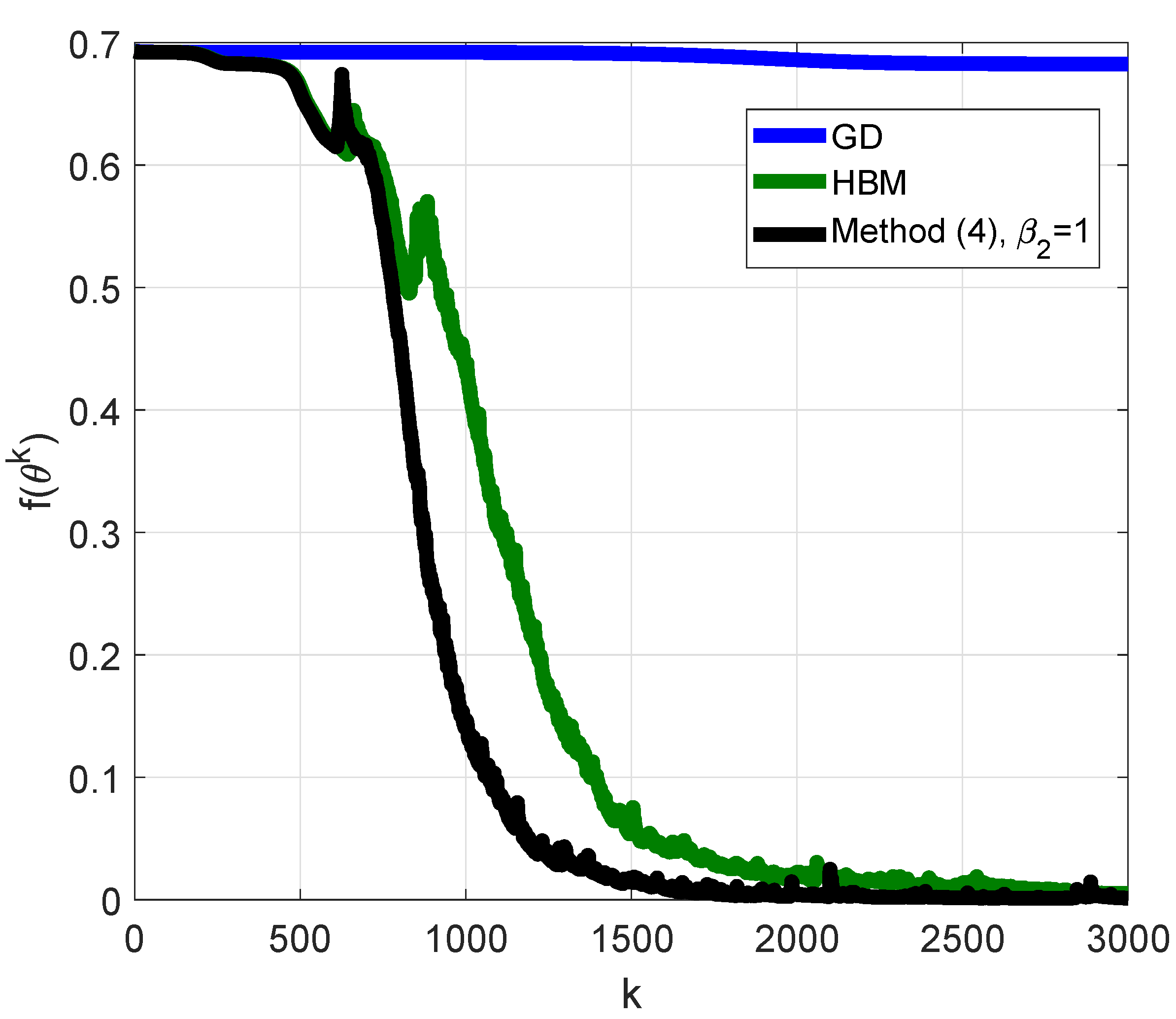
3.8. Recurrent Neural Network
4. Conclusions
- It was demonstrated that, in the case of the quadratic function, method (4) can be easily investigated using the first Lyapunov method. As a result of its application, the convergence conditions presented in Theorem 1 were obtained. Such conditions led to the conditions for the HBM (3) in the case of (see [7]). For functions from , such conditions can be treated as the conditions of local convergence.
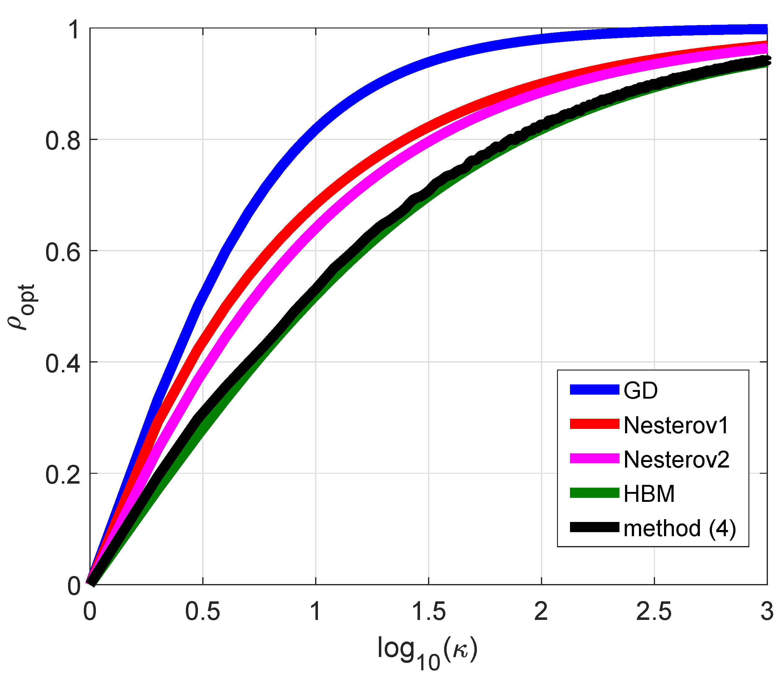
- In comparison with the HBM, optimal parameters for method (4) can only be obtained numerically by the solution of the 3D constrained problems (19) and (20). As demonstrated, for the quadratic case, the optimal value of was equal to zero, so method (4) did not provide additional acceleration in comparison to the standard HBM.
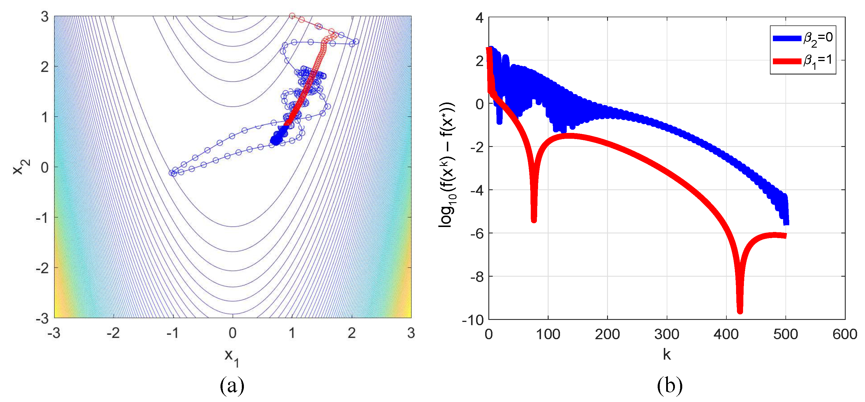
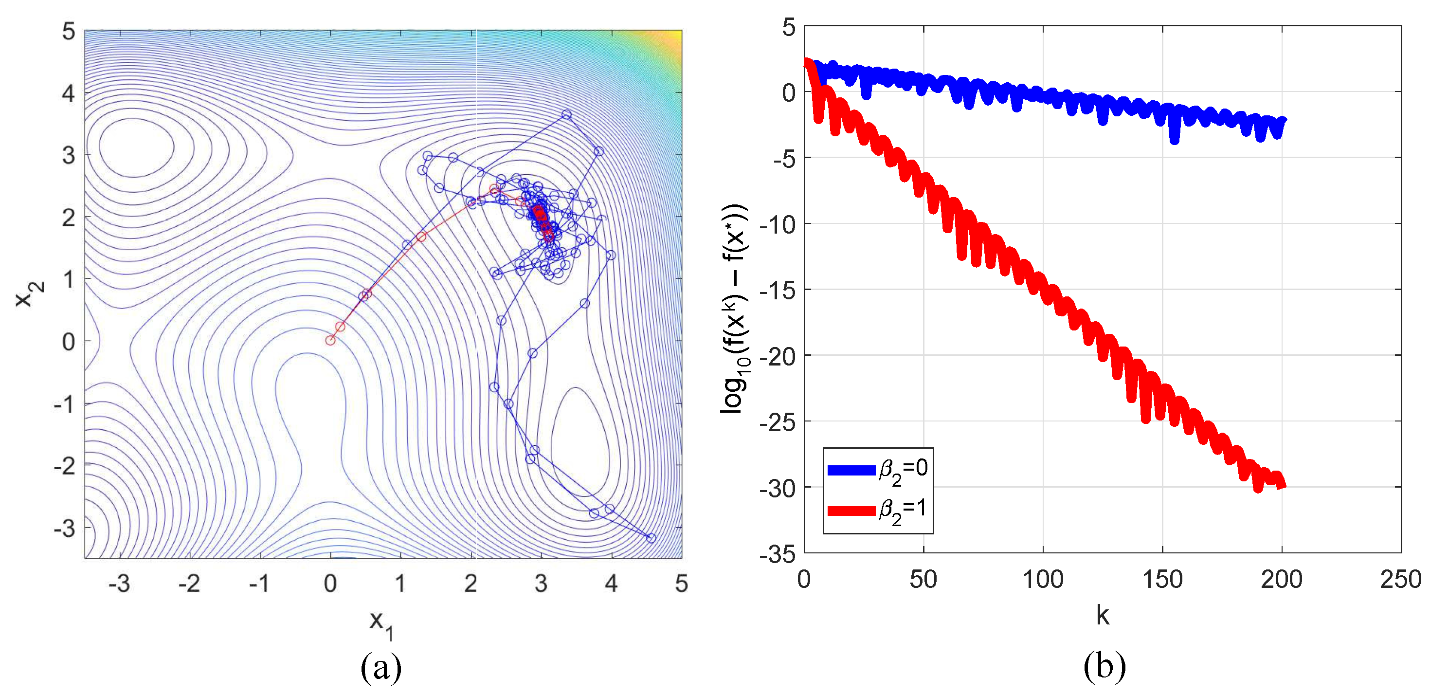
- The ’mechanical’ role of was demonstrated by the consideration of the ODE (25), which is equivalent to (4) in the 1D case. This ODE describes the descent process in the neighborhood of . As can be seen from (25), the presence of realized an additional damping of oscillations associated with non-monotone convergence of the HBM [13].
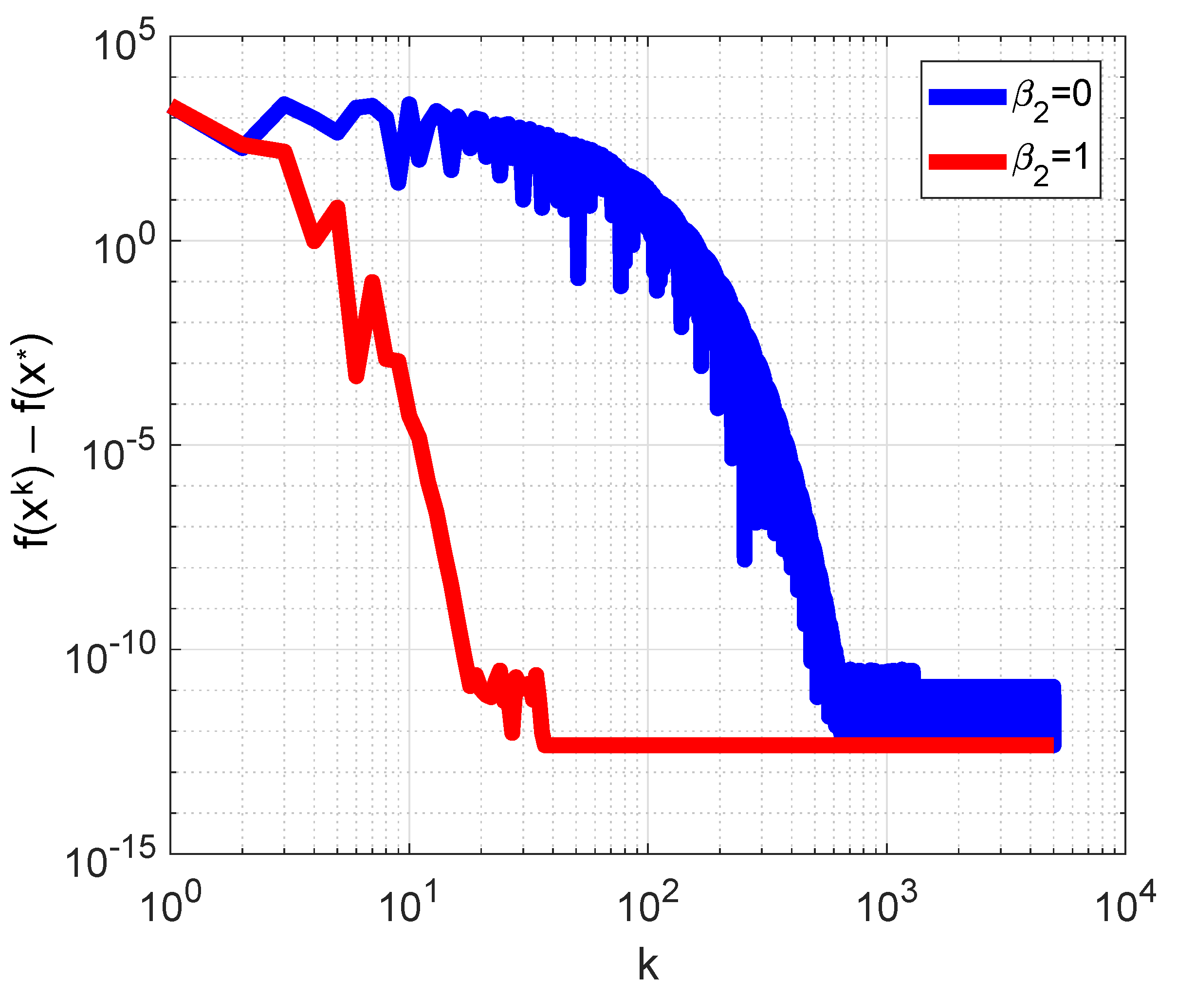
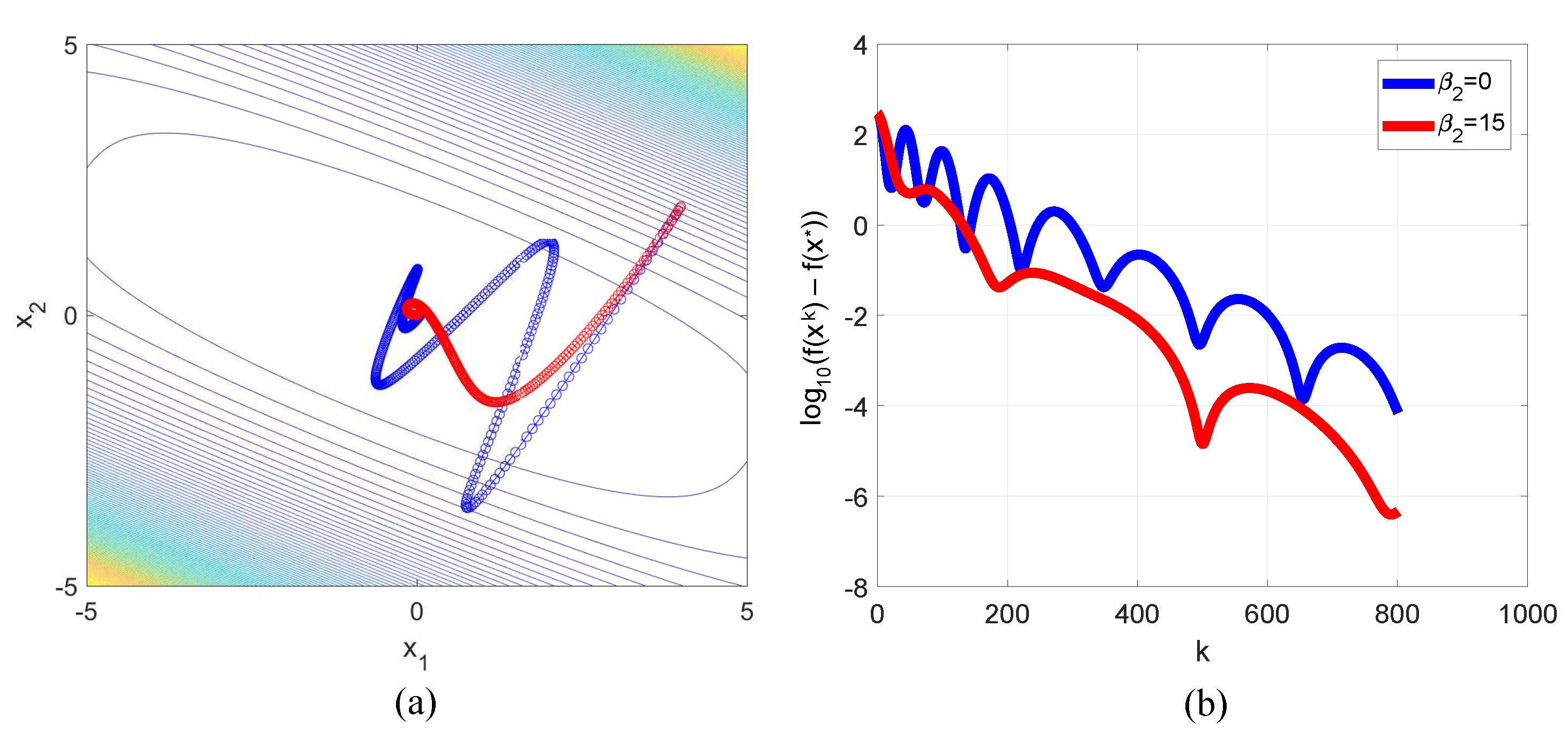
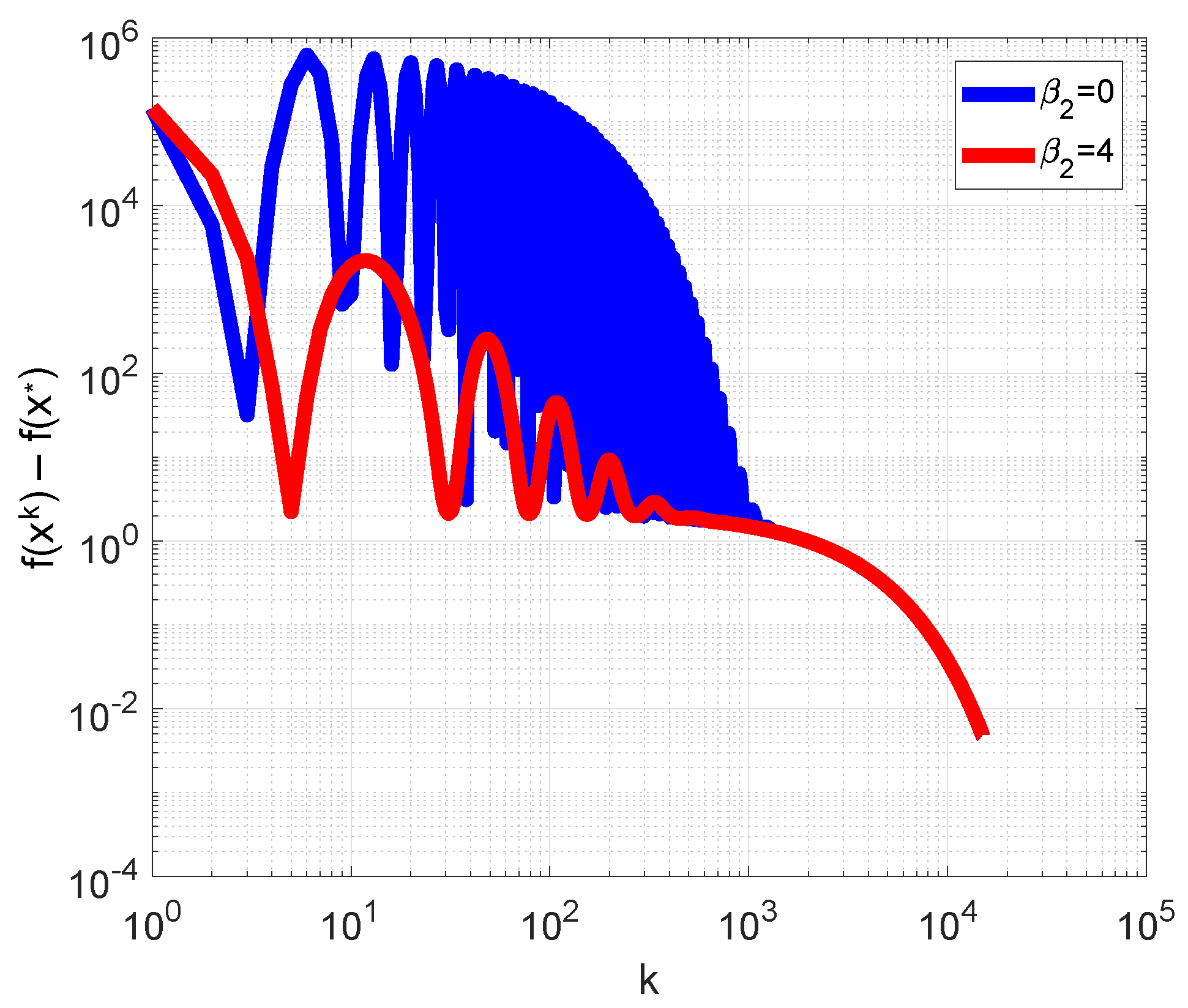
- In numerical examples from different applications, it was demonstrated that, with the use of proper values of , a decrease in oscillation amplitudes typical of the HBM can be realized.
- In this paper, a local convergence analysis was presented. For , global convergence for a specific choice of the parameters was demonstrated in [29]. It is imperative to obtain the general conditions for the parameters that guarantee global convergence.As is known for the HBM (e.g., see [28]), the convergence conditions obtained for strongly convex quadratic functions can lead to a lack of global convergence for .
- An analysis of method (4) was performed for the case of constant values of and . But as known [18], it is effective to use methods with adaptive momentum, whose value is dependent on k in order to improve the convergence. Thus, the construction of extensions of method (4) to the case of adaptive parameters is a perspective for future research.
- In this paper, all methods were considered in their deterministic formulations. However, in modern problems, especially those arising in machine learning, stochastic gradient methods are used according to the size of the datasets. Therefore, the extension of method (4) and its modifications for stochastic optimization has potential for future investigation, especially for applications in machine learning.
Author Contributions
Funding
Data Availability Statement
Acknowledgments
Conflicts of Interest
References
- Bishop, C. Pattern Recognition and Machine Learning; Springer: Berlin, Germany, 2006. [Google Scholar]
- Leonard, D.; van Long, N.; Ngo, V.L. Optimal Control Theory and Static Optimization in Economics; Cambridge University Press: Cambridge, UK, 1992. [Google Scholar]
- Saad, Y. Iterative Methods for Sparse Linear Systems; SIAM: Philadelphia, PA, USA, 2003. [Google Scholar]
- Ljung, L. System Identification: Theory for the User; Prentice Hall PTR: Hoboken, NJ, USA, 1999. [Google Scholar]
- Boyd, S.; Vandenberghe, L. Convex Optimization; Cambridge University Press: Cambridge, UK, 2004. [Google Scholar]
- Nesterov, Y. Introductory Lectures on Convex Optimization: A Basic Course; Springer: Berlin, Germany, 2004. [Google Scholar]
- Polyak, B. Introduction to Optimization; Optimization Software Inc.: New York, NY, USA, 1987. [Google Scholar]
- Polyak, B. Some methods of speeding up the convergence of iteration methods. USSR Comput. Math. Math. Phys. 1964, 4, 1–17. [Google Scholar] [CrossRef]
- Ghadimi, E.; Feyzmahdavian, H.R.; Johansson, M. Global convergence of the heavy-ball method for convex optimization. In Proceedings of the 2015 European Control Conference (ECC), Linz, Austria, 15–17 July 2015; pp. 310–315. [Google Scholar]
- Aujol, J.-F.; Dossal, C.; Rondepierre, A. Convergence rates of the heavy ball method for quasi-strongly convex optimization. SIAM J. Optim. 2022, 32, 1817–1842. [Google Scholar] [CrossRef]
- Bhaya, A.; Kaszkurewicz, E. Steepest descent with momentum for quadratic functions is a version of the conjugate gradient method. Neural Netw. 2004, 17, 65–71. [Google Scholar] [CrossRef] [PubMed]
- Goujaud, B.; Taylor, A.; Dieuleveut, A. Quadratic minimization: From conjugate gradients to an adaptive heavy-ball method with Polyak step-sizes. In Proceedings of the OPT 2022: Optimization for Machine Learning (NeurIPS 2022 Workshop), New Orleans, LA, USA, 3 December 2022. [Google Scholar]
- Danilova, M.; Kulakova, A.; Polyak, B. Non-monotone behavior of the heavy ball method. In Difference Equations and Discrete Dynamical Systems with Applications. ICDEA 2018. Springer Proceedings in Mathematics and Statistics; Bohner, M., Siegmund, S., Simon Hilscher, R., Stehlik, P., Eds.; Springer: Berlin, Germany, 2020; pp. 213–230. [Google Scholar]
- Danilova, M.; Malinovskiy, G. Averaged heavy-ball method. Comput. Res. Model. 2022, 14, 277–308. [Google Scholar] [CrossRef]
- Josz, C.; Lai, L.; Li, X. Convergence of the momentum method for semialgebraic functions with locally Lipschitz gradients. SIAM J. Optim. 2023, 33, 3012–3037. [Google Scholar] [CrossRef]
- Wang, H.; Luo, Y.; An, W.; Sun, Q.; Xu, J.; Zhang, L. PID controller-based stochastic optimization acceleration for deep neural networks. IEEE Trans. Neural Netw. Learn. Syst. 2020, 31, 5079–5091. [Google Scholar] [CrossRef] [PubMed]
- Ma, J.; Yarats, D. Quasi-hyperbolic momentum and Adam for deep learning. In Proceedings of the ICLR 2019: International Conference on Learning Representations, New Orleans, LA, USA, 6–9 May 2019. [Google Scholar]
- Gitman, I.; Lang, H.; Zhang, P.; Xiao, L. Understanding the role of momentum in stochastic gradient methods. In Proceedings of the NeurIPS 2019: Neural Information Processing Systems, Vancouver, BC, Canada, 8–14 December 2019. [Google Scholar]
- Sutskever, I.; Martens, J.; Dahl, G.; Hinton, G. On the importance of initialization and momentum in deep learning. In Proceedings of the International Conference on Machine Learning, PMLR, Atlanta, GA, USA, 17–19 June 2013; Volume 28, pp. 1139–1147. [Google Scholar]
- Kidambi, R.; Netrapalli, P.; Jain, P.; Kakade, S. On the insufficiency of existing momentum schemes for Stochastic Optimization. In Proceedings of the NeurIPS 2018: Neural Information Processing Systems, Montreal, QC, Canada, 2–8 December 2018. [Google Scholar]
- Attouch, H.; Fadili, J. From the ravinemethod to the Nesterov method and vice versa: A dynamical system perspective. SIAM J. Optim. 2022, 32, 2074–2101. [Google Scholar] [CrossRef]
- Attouch, H.; Laszlo, S.C. Newton-like inertial dynamics and proximal algorithms governed by maximally monotone operators. SIAM J. Optim. 2020, 30, 3252–3283. [Google Scholar] [CrossRef]
- He, X.; Hu, R.; Fang, Y.P. Convergence rates of inertial primal-dual dynamical methods for separable convex optimization problems. SIAM J. Control Optim. 2020, 59, 3278–3301. [Google Scholar] [CrossRef]
- Alecsa, C.D.; Laszlo, S.C. Tikhonov regularization of a perturbed heavy ball system with vanishing damping. SIAM J. Optim. 2021, 31, 2921–2954. [Google Scholar] [CrossRef]
- Diakonikolas, J.; Jordan, M.I. Generalized momentum-based methods: A Hamiltonian perspective. SIAM J. Optim. 2021, 31, 915–944. [Google Scholar]
- Yan, Y.; Yang, T.; Li, Z.; Lin, Q.; Yang, Y. A unified analysis of stochastic momentum methods for deep learning. In Proceedings of the Twenty-Seventh International Joint Conference on Artificial Intelligence (IJCAI-18), Stockholm, Sweden, 13–19 July 2018. [Google Scholar]
- Van Scoy, B.; Freeman, R.; Lynch, K. The fastest known globally convergent first-order method for minimizing strongly convex functions. IEEE Control Syst. Lett. 2018, 2, 49–54. [Google Scholar] [CrossRef]
- Lessard, L.; Recht, B.; Packard, A. Analysis and design of optimization algorithms via integral quadratic constraints. SIAM J. Optim. 2016, 26, 57–95. [Google Scholar] [CrossRef]
- Cyrus, S.; Hu, B.; Van Scoy, B.; Lessard, L. A robust accelerated optimization algorithm for strongly convex functions. In Proceedings of the 2018 Annual American Control Conference (ACC), Milwaukee, WI, USA, 27–29 June 2018. [Google Scholar]
- Gantmacher, F.R. The Theory of Matrices; Chelsea Publishing Company: New York, NY, USA, 1984. [Google Scholar]
- Gopal, M. Control Systems: Principles and Design; McGraw Hill: New York, NY, USA, 2002. [Google Scholar]
- Su, W.; Boyd, S.; Candes, J. A differential equation for modeling Nesterov’s accelerated gradient method: Theory and insights. J. Mach. Learn. Res. 2016, 17, 1–43. [Google Scholar]
- Luo, H.; Chen, L. From differential equation solvers to accelerated first-order methods for convex optimization. Math. Program. 2022, 195, 735–781. [Google Scholar] [CrossRef]
- Eftekhari, A.; Vandereycken, B.; Vilmart, G.; Zygalakis, K.C. Explicit stabilised gradient descent for faster strongly convex optimisation. BIT Numer. Math. 2021, 61, 119–139. [Google Scholar] [CrossRef]
- Fountoulakis, K.; Gondzio, J. A second-order method for strongly convex ℓ1-regularization problems. Math. Program. 2016, 156, 189–219. [Google Scholar] [CrossRef]
- Scieur, D.; d’Aspremont, A.; Bach, F. Regularized nonlinear acceleration. Math. Program. 2020, 179, 47–83. [Google Scholar] [CrossRef]


Disclaimer/Publisher’s Note: The statements, opinions and data contained in all publications are solely those of the individual author(s) and contributor(s) and not of MDPI and/or the editor(s). MDPI and/or the editor(s) disclaim responsibility for any injury to people or property resulting from any ideas, methods, instructions or products referred to in the content. |
© 2024 by the authors. Licensee MDPI, Basel, Switzerland. This article is an open access article distributed under the terms and conditions of the Creative Commons Attribution (CC BY) license (https://creativecommons.org/licenses/by/4.0/).
Share and Cite
Krivovichev, G.V.; Sergeeva, V.Y. Analysis of a Two-Step Gradient Method with Two Momentum Parameters for Strongly Convex Unconstrained Optimization. Algorithms 2024, 17, 126. https://doi.org/10.3390/a17030126
Krivovichev GV, Sergeeva VY. Analysis of a Two-Step Gradient Method with Two Momentum Parameters for Strongly Convex Unconstrained Optimization. Algorithms. 2024; 17(3):126. https://doi.org/10.3390/a17030126
Chicago/Turabian StyleKrivovichev, Gerasim V., and Valentina Yu. Sergeeva. 2024. "Analysis of a Two-Step Gradient Method with Two Momentum Parameters for Strongly Convex Unconstrained Optimization" Algorithms 17, no. 3: 126. https://doi.org/10.3390/a17030126