1. Introduction
Zero-order methods are usually applied to problems in which the function being optimized has no explicit analytic expression. To calculate the values of such functions, it is necessary to solve non-trivial auxiliary problems of computational mathematics and optimization. In some cases, it is assumed that the calculation of a single objective function value may take from a few minutes to several hours of continuous computer operation. Developing an effective global optimization method requires identifying certain properties of the objective function (and constraints), for example, determining a good estimate of the Lipschitz constant [
1,
2,
3,
4] or representing a function as a difference between two convex functions [
5,
6,
7]. Such auxiliary problems do not always have a unique solution and are not often easily solvable. The effectiveness of global optimization methods often depends on the ability to quickly find a good local solution [
8], which can significantly speed up some global optimization methods (for example, the branch and bounds method).
The aim of the paper is to test several well-known zero-order methods on nonconvex global optimization problems a using special version of the multistart strategy. We check the ability of these methods not only to find a good local solution but also to find a global optimum of the problem. The multistart strategy was considered as a starting case for population-based optimization. It is necessary to note that the multistart approach can be considered as an overabundant population. Our aim is to check the efficiency of the suggested approach under this condition.
Special attention is given to the Parabola Method in the present work. The reason for such an investigation is the following: if the objective function is differentiable, then in a small neighborhood of an interior local minimum point, the objective function behaves like a convex function. In [
9], a more general statement of this property based on the concept of local programming is given. A combination of this method with different zero-order methods in multivariate optimization problems demonstrates quite high performance and global optimization method qualities. We tested several well-known zero-order multivariate optimization methods; nevertheless, application of this modification of the Parabola Method as the line-search procedure can be used in many other methods.
The paper is organized as follows. In
Section 2, we give a description of the Golden Section and Parabola Methods and perform numerical experiments on a set of univariate optimization problems. A numerical comparison of zero-order methods in combination with the Golden Section and Parabola Methods is presented in
Section 3. We conclude the paper with a short discussion of the results in
Section 4 and
Section 5.
2. Univariate Optimization: Parabola Method
We consider the following optimization problem
where
is a continuously differentiable function. It is assumed that
f has a finite number of local minima over
P, and only values of
f are available. Problems with such an assumption are described in [
10]. In this section, we consider two well-known univariate optimization methods: the Golden Section Method (GSM) [
11] and the Quadratic Interpolation Method or the Powell M.J.D. Method or the Parabola Method (PM) [
12]. Let us give brief descriptions of both methods.
2.1. The Golden Section Method
- Step 0.
Choose the accuracy of the algorithm . Set . Evaluate and . Set .
- Step 1.
If , stop: is -optimal point. Otherwise, if , go to Step 2; else, go to Step 3.
- Step 2.
Set Evaluate . Go to Step 4.
- Step 3.
Set . Evaluate . Go to Step 4.
- Step 4.
Increase , and go to Step 1.
2.2. The Parabola Method
- Step 0.
Choose the accuracy
. Choose points
such that
Set .
- Step 1.
Find the minimum
of the quadratic interpolation polynomial in the following way.
- Step 2.
If (
3) is held, then terminate the algorithm, and
is
-optimal point. Otherwise, go to Step 3.
- Step 3.
Choose .
Set . Denote points in ascending order as . Increase , and go to Step 1.
When
f is a unimodal (semi-strictly quasiconvex [
13]) over
P function, both methods determine an approximate point of minimum in a finite number of iterations. In the case of the Golden Section Method the number of function evaluations is equal to the number of iterations plus two; in the case of the Parabola Method, the number of function evaluations is equal to the number of iterations plus three. It is well known that, in general, the Golden Section Method is more efficient than the Parabola Method. However, in the continuously differentiable case, the behavior of the Parabola Method can be improved.
Consider the following two examples from [
14].
Example 1. In problem (1), . The Golden Section Method with finds the approximate solution with in 16 iterations. The Parabola Method with the same ε finds the approximate solution with in six iterations. Example 2. In problem (1), . The Golden Section Method with finds the approximate solution with in 19 iterations. The Parabola Method with the same ε finds the approximate solution with in 35 iterations. In both examples, the objective functions are unimodal. In the first example, the Parabola Method worked two times faster, and in the second example, the Parabola Method worked about two times slower than the Golden Section Method. From a geometrical point of view, the objective function in the first example is more like a parabola than in the second example, and we are going to show how the efficiency of the Parabola Method can be improved in cases similar to Example 2.
We start from checking efficiency of the Golden Section Method on a number of multimodal functions.
Table 1 and
Table 2 present the results of 17 test problems from [
14].
The sign g in the g/l column corresponds to the case when a global minimum point was determined, and the sign l corresponds to the case when only a local minimum point was determined. Symbol corresponds to the number of function evaluations. Surprisingly enough, only in four problems was a local minimum determined; in all other problems, the Golden Section Method found global solutions.
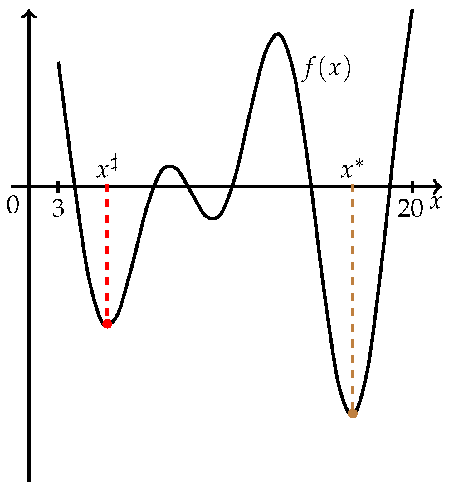
The geometrical interpretation of failure of the Golden Section Method in finding a global minimum can be given on the basis of problems 7 and 11 from
Table 2. In these cases, only local minimum points were determined, and, as can be seen from
Figure 1 and
Figure 2, the global minimum points are located closer to the endpoints of the feasible intervals. Hence, we can make the following assumption: univariate multimodal problems with global minimum points located more or less in the middle of the intervals are more efficiently tractable by the Golden Section Method from the global optimization point of view. This topic needs further theoretical investigation and is not the subject of our paper.
Let us turn now to the Parabola Method. In order to start the method, property (
2) must be satisfied. The points satisfying property (
2) are known as a three-point pattern (TPP) in [
11]. In order to find the TPP, we propose the following procedure.
2.3. TPP Procedure
- Step 0.
Choose integer , and calculate . Set .
- Step 1.
Calculate .
- Step 3.
If , then .
- Step 4.
If , then increase , and go to Step 1. Otherwise, stop.
When the TPP procedure stops, we have three-point patterns, and in order to find the best solution, we can start the Parabola Method for all patterns. In practice, we used the TPP procedure several times. We started from a small enough value of N, say , and ran the TPP procedure. Then, we increased and ran the TPP procedure again. When the number of three-point patterns was the same in both runs, we stopped. In this case, we say that the TPP procedure stabilized. Otherwise, we increased N and ran the TPP procedure again, and so on. Since we assumed that the number of local minima of f over P is finite, such a repetition is also finite. Finally, we obtained TPP subintervals and the three-point corresponding patterns , . We cannot guarantee that each subinterval contains exactly one local minimum; but, in practice, this property is true rather often. Then, we ran the Parabola Method for each subinterval, found the corresponding local minima, and selected the best ones as solutions. If , then no three-point patterns were detected. In this case, the Parabola Method is not applicable (it can be disconvergent), and we switch to the Golden Section Method. We call this strategy a two-stage local search approach (two-stage approach for short).
Let us apply the two-stage approach to solving problems 11 (
Figure 1) and 7 (
Figure 2) from
Table 1 for which the Golden Section Method did not find global minimum points and then run the Parabola Method over each obtained subinterval.
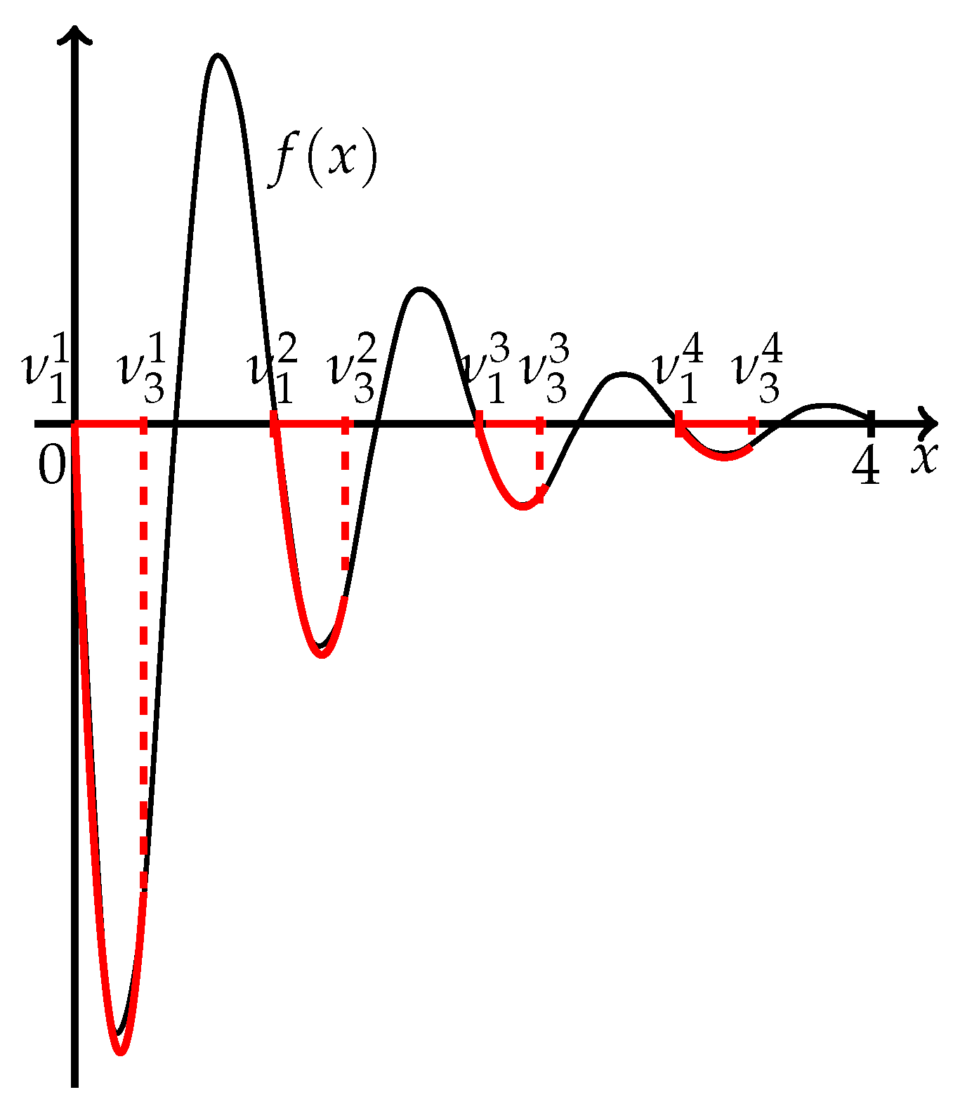
Example 3. Problem 11: . Initial value . The TPP procedure was run four times. After the first run, one subinterval with one three-point pattern was obtained, after the second run, two subintervals with two three-point patterns were obtained, after the third run, four subintervals with four three-point patterns were obtained, and after the fourth run, four smaller subintervals with four three-point patterns were obtained again. The TPP procedure was stopped, and . The total number of function evaluations was equal to 24. Then, with the accuracy , we ran the Parabola Method, which stopped after two additional function evaluations for each subinterval. The final subintervals, the three-point pattern (TPP), the corresponding starting parabolas, and additional function evaluations () of the Parabola Method over each subinterval are given in Table 3. Therefore, in total, after 32 function evaluations, all minima of the given function were determined. The geometrical interpretation of the results of the TPP procedure application corresponding to
Table 3 is presented in
Figure 3.
Example 4. Problem 7: . Initial value . Three subintervals were determined after four runs of the TPP procedure, (see Figure 4). The results of the TPP procedure and the Parabola Method are given in Table 4. After 36 function evaluations, all minima were detected.
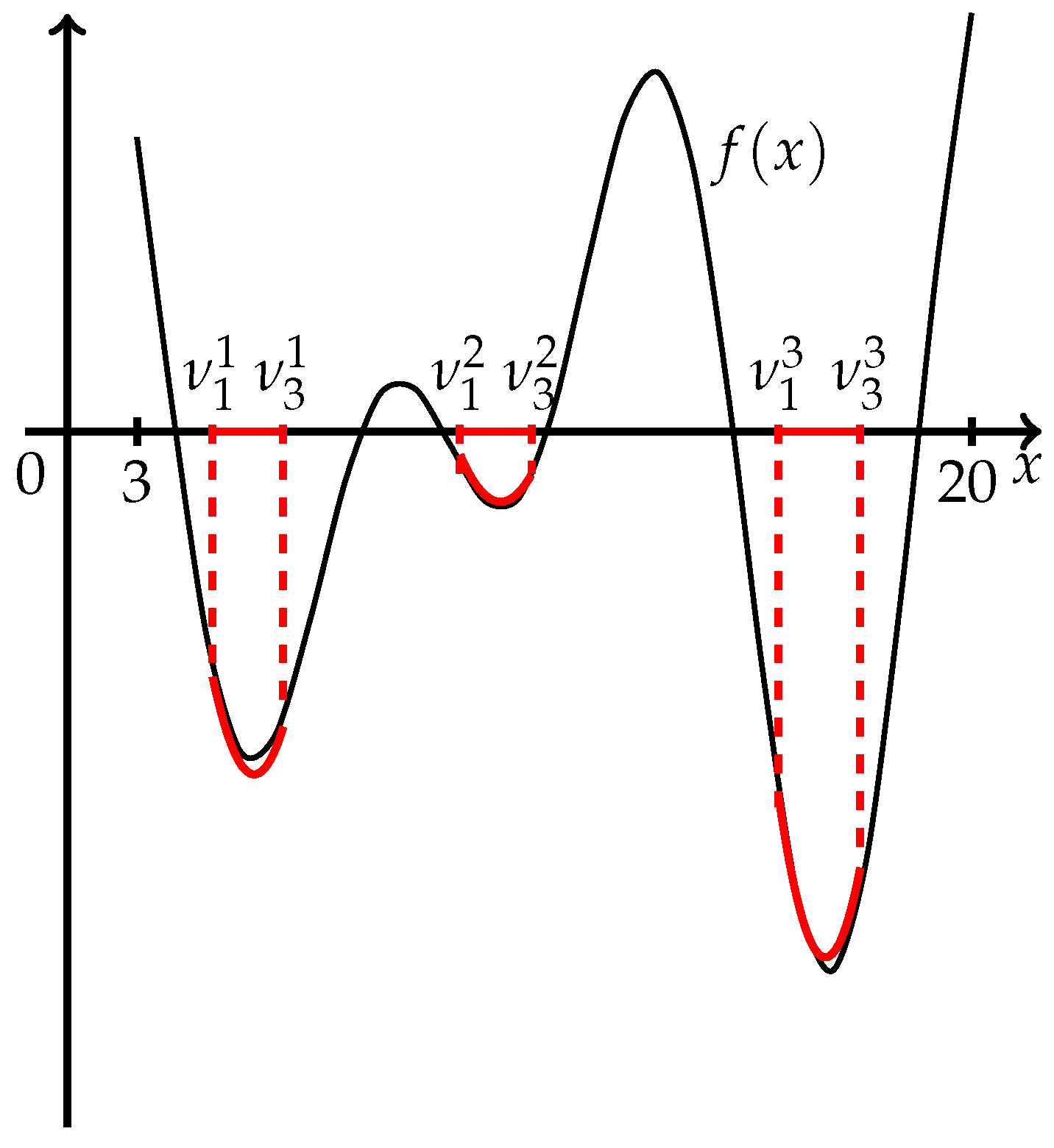
Now, we apply the two-stage approach to the problems from
Table 1 and
Table 2. The results are given in
Table 5 and
Table 6. Since problems 7 and 11 were considered in Examples 3 and 4, they are not included in the
Table 5. Problem 6 is described in
Table 5.
In these tables, the Minima structure column shows how many local and global minima each problem has, the column shows the number of performed function evaluations until the TPP procedure is stabilized, the TPP subintervals column shows the subintervals obtained from application of the TPP procedure, the column shows the number of function evaluations of the Golden Section Method, the column shows the number of function evaluations of the Parabola Method, and the g/l column shows the type of the calculated point: g—global minimum, l—local minimum. For example, for problem 2 with two local minima and one global minima, the TPP procedure found three subintervals after 12 function evaluations. The first subinterval contains a local minimum, the second subinterval contains a global minimum, and the third subinterval contains a local minimum. The minimum over the first subinterval was found by the Golden Section method in 14 function evaluations and by the Parabola Method in 4 function evaluations. The same results from both methods were demonstrated over the second and the third subintervals. Therefore, the total number of function evaluations spent by the two-stage approach with the Golden Section Method at the second stage was and function evaluations with the Parabola Method.
Table 6 shows the results of the application of the two-stage approach to problem 6. Application of the TPP procedure finished in 19 subintervals, and for each of them, the Golden Section Method and the Parabola Method were used; all global minima were found, as well as all interior local minima, and one local minimum was attained at the endpoint of the feasible interval.
We can see from the presented test results that the direct application of the two-stage approach may involve a lot of computation. If we are interested in finding a good local solution faster than the pure Golden Section Method we can use the following Accelerated Two-Stage Approach (ATSA).
3. Accelerated Two-Stage Approach
In this section, we propose a modification of the two-stage approach described in the previous section. We set the integer parameter
N in the TPP procedure in advance and do not change it. When the TPP procedure is finished,
values of the objective function at points
with
are available. We determine the record value
and a corresponding record point
. If the number
of the TPP subintervals is positive,
, then we choose the TPP subinterval, which contains the record point
, and run the Parabola Method over this TPP subinterval. Let
be a point found by the Parabola Method. We define the point
and the corresponding objective value
. We deliver the pair
as the result of the Accelerated Two-Stage Approach. If the number
is equal to zero, i.e., no TPP subintervals were detected, then we determine
and run the Golden Section Method over the interval
. Let
be the corresponding point determined by the Golden Section Method. As in the previous case, we define the point
and the value
, and we deliver the pair
, as a result of the Accelerated Two-Stage Approach (ATSA).
Let us now give the description of the ATSA procedure.
The ATSA Procedure
- Step 1.
Apply the TPP procedure. Let and be parameters calculated by the TPP procedure. Let be the record value over all calculated points and .
- Step 2.
If , then select the subinterval containing and run the Parabola Method over the selected subinterval, obtaining the point . Define the point and value . Stop.
- Step 3.
If
, then determine the subinterval
according to (
4) and run the Golden Section Method, obtaining the point
. Define the point
and value
. Stop.
The results of testing the accelerated two-stage approach are given in
Table 7. The integer parameter
N for the TPP procedure was equal to 3. The GSM/PM column shows the number of function evaluations of the corresponding method. If, after the first stage, the number of TPP subintervals was equal to zero (as for problem 1
), then the Golden Section Method was used, and the number of function evaluations
. If, after the first stage, the number of the TPP subintervals was positive (as for problem 2
), then the Parabola Method was used, and the number of function evaluations
. The Total
column shows the total number of function evaluations of the ATSA procedure, and the g/l column shows a global (g) or local (l) minimum was found.
We have to mention that the integer parameter N (the number of the subdivision points in the TPP procedure) is the most crucial. If, for example, N is equal to 20, then for all testing problems, global minimum points were determined. However, in this case, the numbers of objective function evaluations were rather large, more than several tens. The parameter N can be chosen according to the number of expected local minima. In the general case, we aim to find a good local minimum, and from the results of our testing, we recommend choosing an N between 5 and 10.
We can see from
Table 7 that the accelerated two-stage approach finds solutions with lower computational efforts compared to the pure Golden Section Method, still finding global solutions in almost all the test problems. As for problems 12 and 17, some further modifications can be invented. Nevertheless, the current results are encouraging.
4. Numerical Comparison of Zero-Order Methods: Multivariate Optimization Problems
We tested and compared the following zero-order methods: the Hooke and Jeeves method combined with the ATSA, the Rosenbrock method with a discrete step in the search procedure, the Rosenbrock method combined with the ATSA, and the coordinate descent method combined with the ATSA. In the current section, we give a brief description of these methods. Many of them are described in monographs and review articles on optimization methods [
10,
11,
15,
16,
17,
18,
19].
Hooke and Jeeves method. The pattern search method of Hooke and Jeeves consists of a sequence of exploratory moves about a base point that, if successful, are followed by pattern moves.
The exploratory moves acquire information about the function in the neighborhood of the current base point . Each variable , in turn, is given an increment (first, in the positive direction and then, if necessary, in the negative direction), and a check is made of the new function value. If any move results in a reduced function value, the new value of that variable will be retained. After all the variables have been considered, a new base point will be reached. If = , no function reduction has been achieved. The step length is reduced, and the procedure is repeated. If , a pattern move from is made.
A pattern move attempts to speed up the search by using the information already acquired about to identify the best search direction. A move is made from in the direction , since a move in this direction leads to a decrease in the function value. In this step, we use the ATSA to solve a univariate optimization problem and obtain a new point . The search continues with a new sequence of exploratory moves about . If the lowest function value obtained is less than , then a new base point has been reached. In this case, a second pattern move is made. If not, the pattern move from is abandoned, and we continue with a new sequence of exploratory moves about .
Rosenbrock method. The main idea of the method is to iteratively find the descending direction of a function along linearly independent and orthogonal directions. A successful step in the current direction leads to an increase in this step on the following iteration by means of a stretch coefficient ; otherwise, the coefficient is used to decrease the step. The search within the current direction system is implemented until all possibilities of function reduction are exhausted. If there are no successful directions, a new set of linearly independent and orthogonal directions is constructed by means of rotating the previous ones in an appropriate manner. To obtain a new direction system, the Gram–Schmidt procedure is used.
Iterative coordinate descent method. This method is a simplified version of the Hooke and Jeeves method. It uses only the analogue of exploratory moves with an appropriate step size obtained from the line search procedure along the current basis vector.
Combined versions. We designed three modifications of the described methods to estimate the potential for finding the global optimum. The iterative coordinate descent method, the Hooke and Jeeves method, and the Rosenbrock method are combined with the ATSA and presented in this section. The following test problems were used to perform numerical experiments.
Global optimum: , , .
Global optimum: , , .
The function has 760 local minimum points for , 18 of them are global optimum points, and .
This function has three minimums for , one of them is global: , and .
The 6-hump camel function has six minimum points for , two of them are global optima: , , and .
The only global minimum of the function is , and .
The function has approximately local minima for , the global minimum is , , and .
As with Levy-2 function, the function has approximately local minima for , the global minimum is , , and .
This function has approximately local minima for , the only global minimum is , , and .
The results of the numerical experiments are presented in
Table 8 and
Table 9. The following notations are used:
n is the number of variables;
is the best value of the objective function found during the executing of the algorithm;
is the optimal value of the objective function;
is the average number of function calculations during the execution of the algorithm considering all launches of the current problem;
m is the number of problems solved successfully using the multistart procedure;
M is the total number of randomly generated points. The multistart procedure launches the algorithm from one of the generated points. The designation
means that
m launches of the algorithm from
M starting points resulted in a successful problem solution (the global minimum point was found). Coordinate descent–par is the coordinate descent method in combination with the ATSA; Hooke–Jeeves–par is the Hooke and Jeeves method combined with the ATSA; Rosenbrock–dis is the Rosenbrock method with a discrete step in the search procedure; Rosenbrock–par is the Rosenbrock method in combination with the ATSA.
5. Discussion of the Results
The coordinate descent method in combination with the ATSA proved to be an effective method in searching for the global optimum even in quite difficult optimization problems. For instance, notice the results for Levy functions. Despite the large number of local minima in the search area of these functions, the algorithm in most cases found the global minimum points. The coordinate descent method in combination with the ATSA demonstrated an acceptable number of function calculations and quite high accuracy of the best function value for all tested problems.
The Hooke and Jeeves method combined with the ATSA attained global optimum points in most tested problems but not as frequently as the coordinate descent method. Nevertheless, it is possible to obtain quite a high accuracy of the best-found solution for some problems. The price for this accuracy is a large number of objective function calculations due to the careful selection of start points in the ATSA.
The Rosenbrock method with the ATSA has the same obvious drawback as the Hooke and Jeeves method, namely, the number of function calculations is quite large. However, we can notice that the Rosenbrock method with a discrete step demonstrated acceptable performance considering the number of successive launches and function calculations.
6. Conclusions
We tested some of the well-known zero-order methods and added to their algorithms a line search based on the ATSA for univariate problems. Some of the tested problems, for instance, the Shubert problem and Levy problems are quite difficult in terms of searching for the global optimum; however, according to the numerical experiments, it is possible to use zero-order methods to find the global optimum with quite high accuracy and with acceptable performance. The coordinate descent method combined with the ATSA deserves attention in terms of its ability to find a global optimum with high frequency in most tested problems.
It would be very interesting to combine the suggested Parabola Method with other zero-order methods like the Downhill Simplex, Genetic Algorithm, Particle Swarm Optimization, Cuckoo Search Algorithm, and the YUKI algorithm. We will continue our investigations and are working on a new paper devoted to such extension and testing.


