
Model Predictive Evolutionary Temperature Control via Neural-Network-Based Digital Twins

Abstract
:1. Introduction
2. Materials and Methods
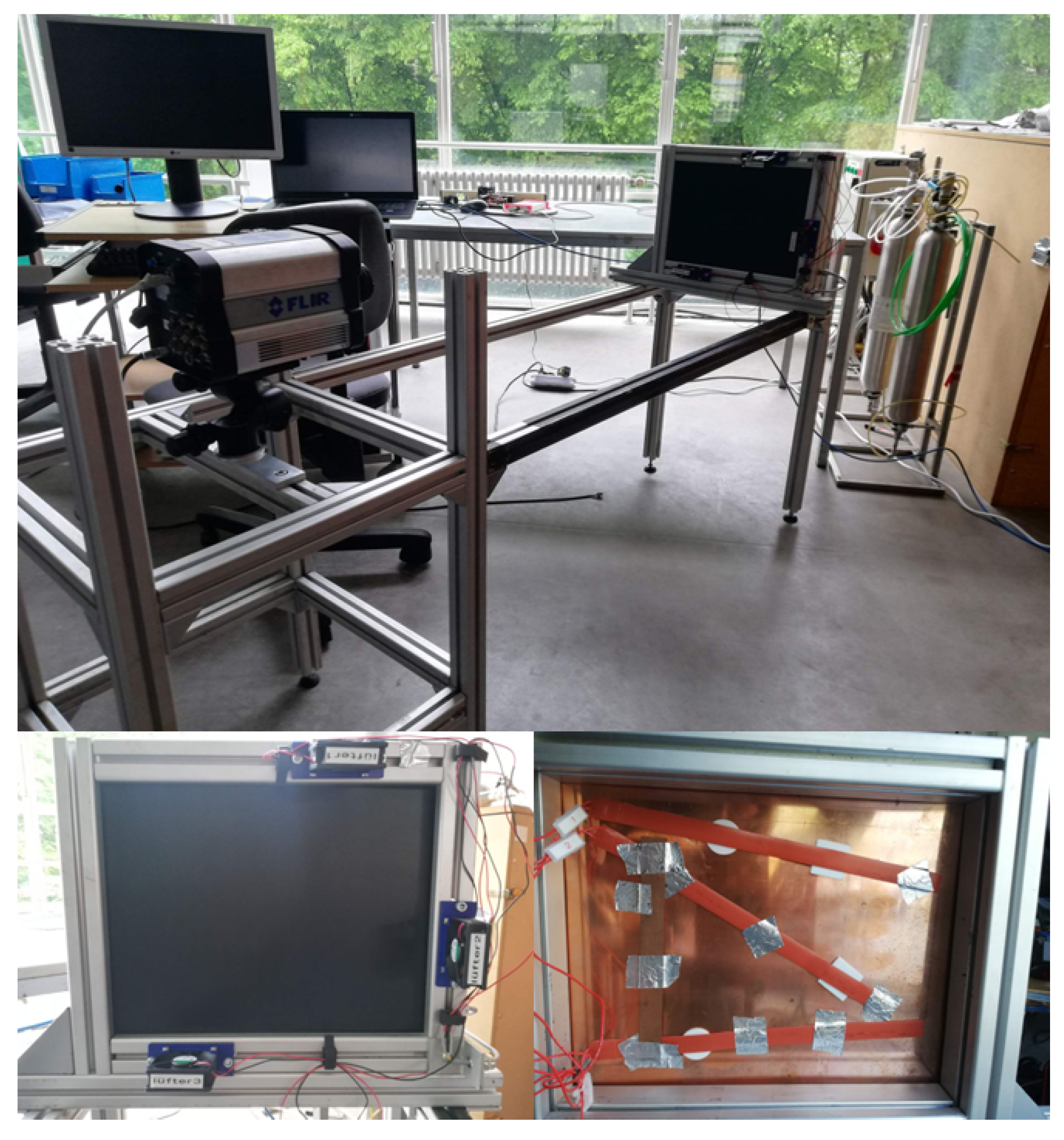
2.1. Experimental Setup
- A copper plate—selected due to its high thermal conductivity in order to reduce the duration of the experiments;
- The copper plate is coated with a high-emissivity black paint (Nextel Velvet Coating 811-21) for improved signal-to-noise ratio;
- Three heating strips on the backside of the plate arranged in a “Z”-like pattern—310 mm × 17 mm, 24 , 36 ;
- Three fans located on the perimeter of the plate—SUNON, 12 , ;
- A data acquisition module (myDAQ, NI) with an in-house built control unit;
- A mid-wave infrared camera—FLIR SC5000, (512 × 640) pixels;
- A LabVIEW interface for the real-time control of the system.
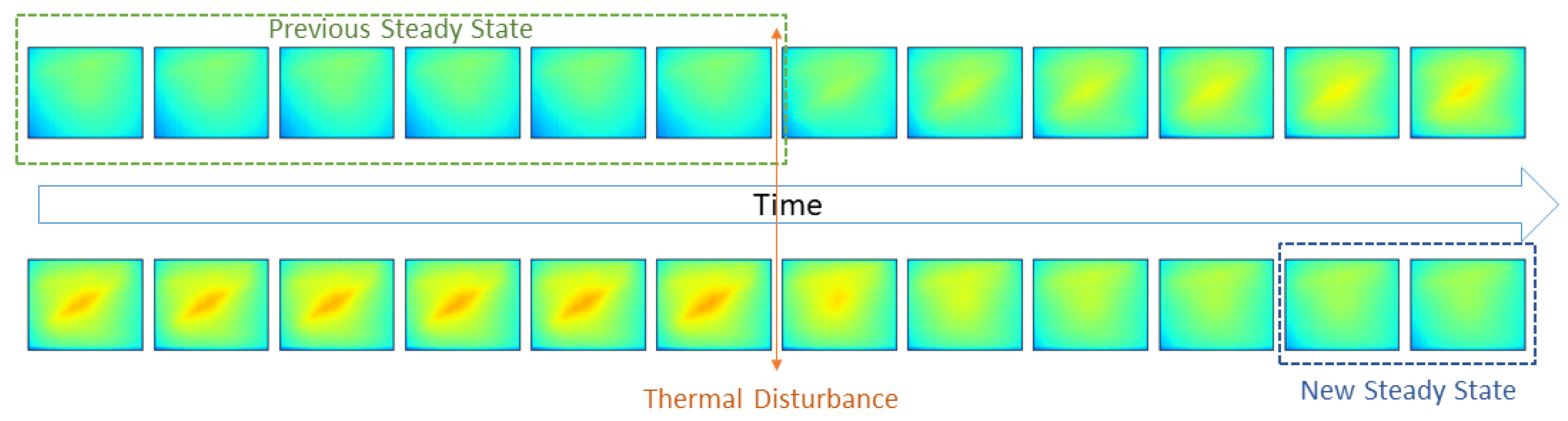
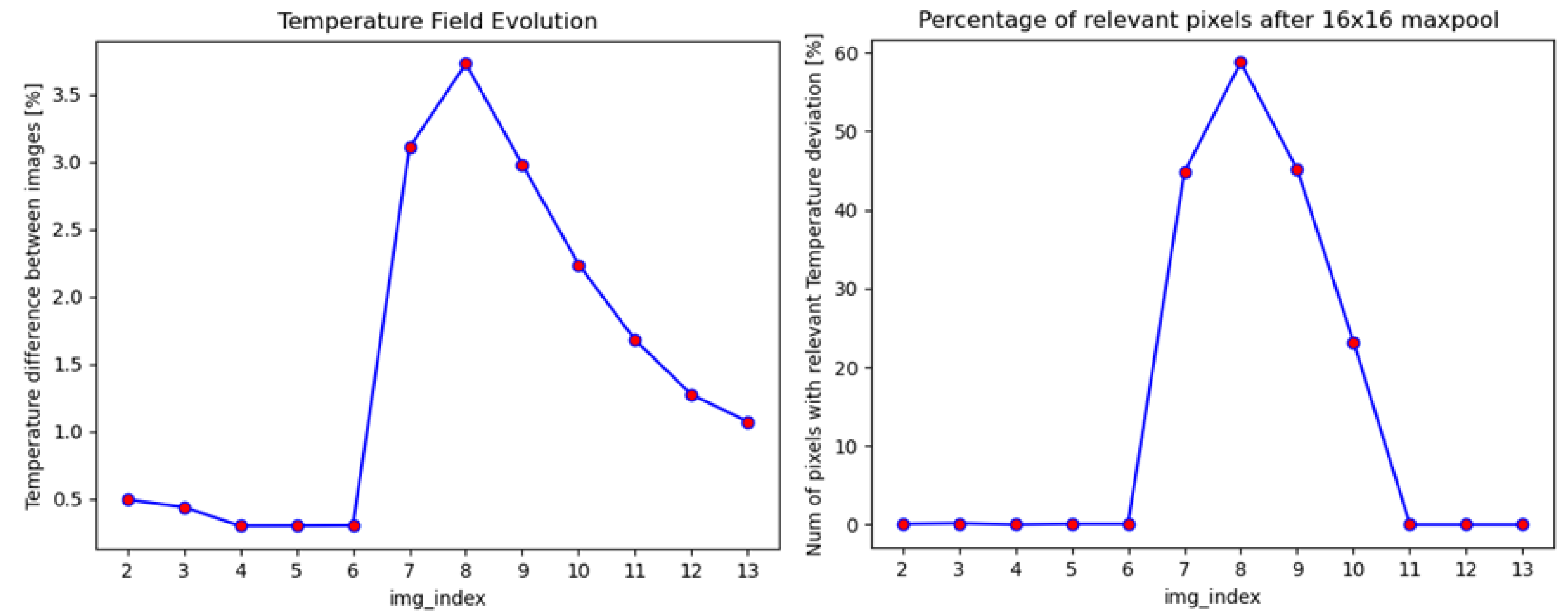
- The per pixel percentage difference of consecutive frames after 16 × 16 max filter is less than 1.5%. The application of this max filter is required for two reasons. First, due to thermal inertia, the difference between consecutive frames can be small, and thus we increase the rigidity of the steady-state condition. Second, we reduce the impact of objects that have the same temperature in all frames (e.g., the frame around the plate).
- The pixels with a 3% deviation in consecutive frames are less than 1% of the total pixels in a frame after a max filter.
2.2. Dataset
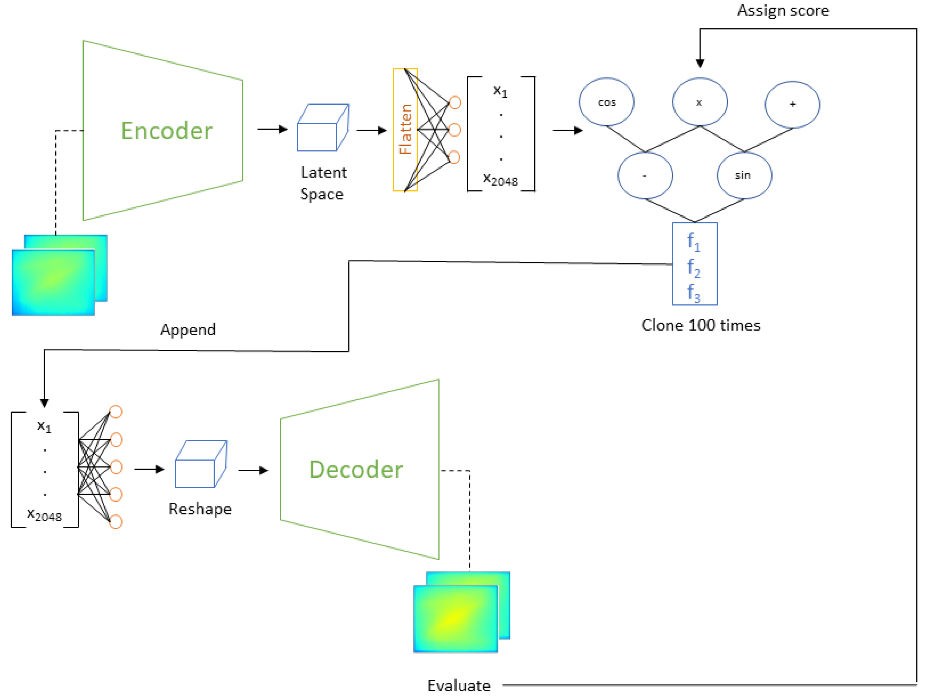
2.3. Digital Twin
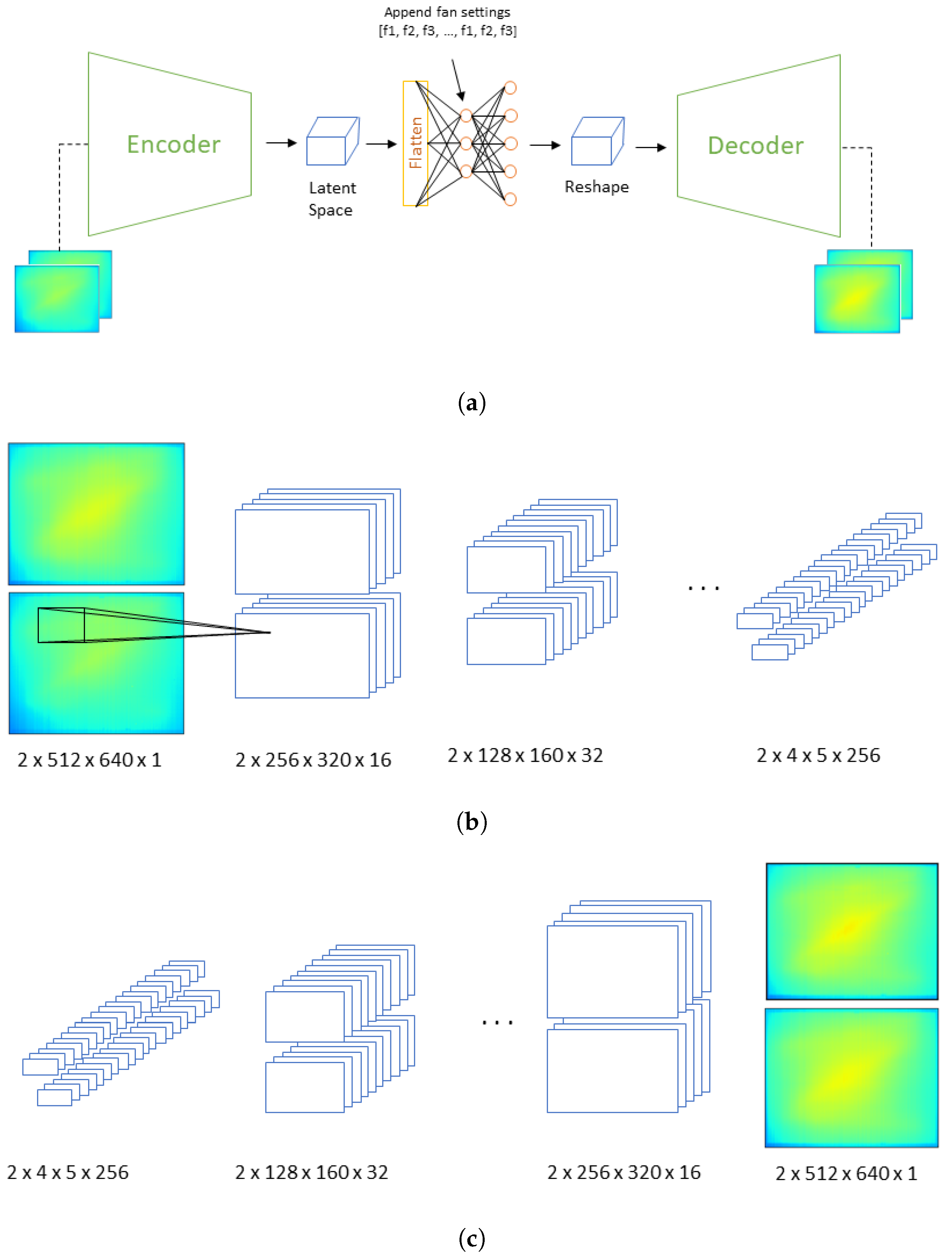
2.3.1. Model Architecture
2.3.2. Training Protocol
- The batch size was set to 16.
- The optimizer employed was Adam, utilizing a default initial learning rate of 0.001.
- A learning rate decay scheme was employed, wherein was initiated after the tenth epoch, with decay continuing until a minimum value of 0.000001 was reached.
- Training was conducted for 800 epochs on an NVIDIA GeForce RTX 3080 GPU. Early stopping was implemented with a patience of 100 epochs.
- One hundred copies of the fan settings vector were utilized.
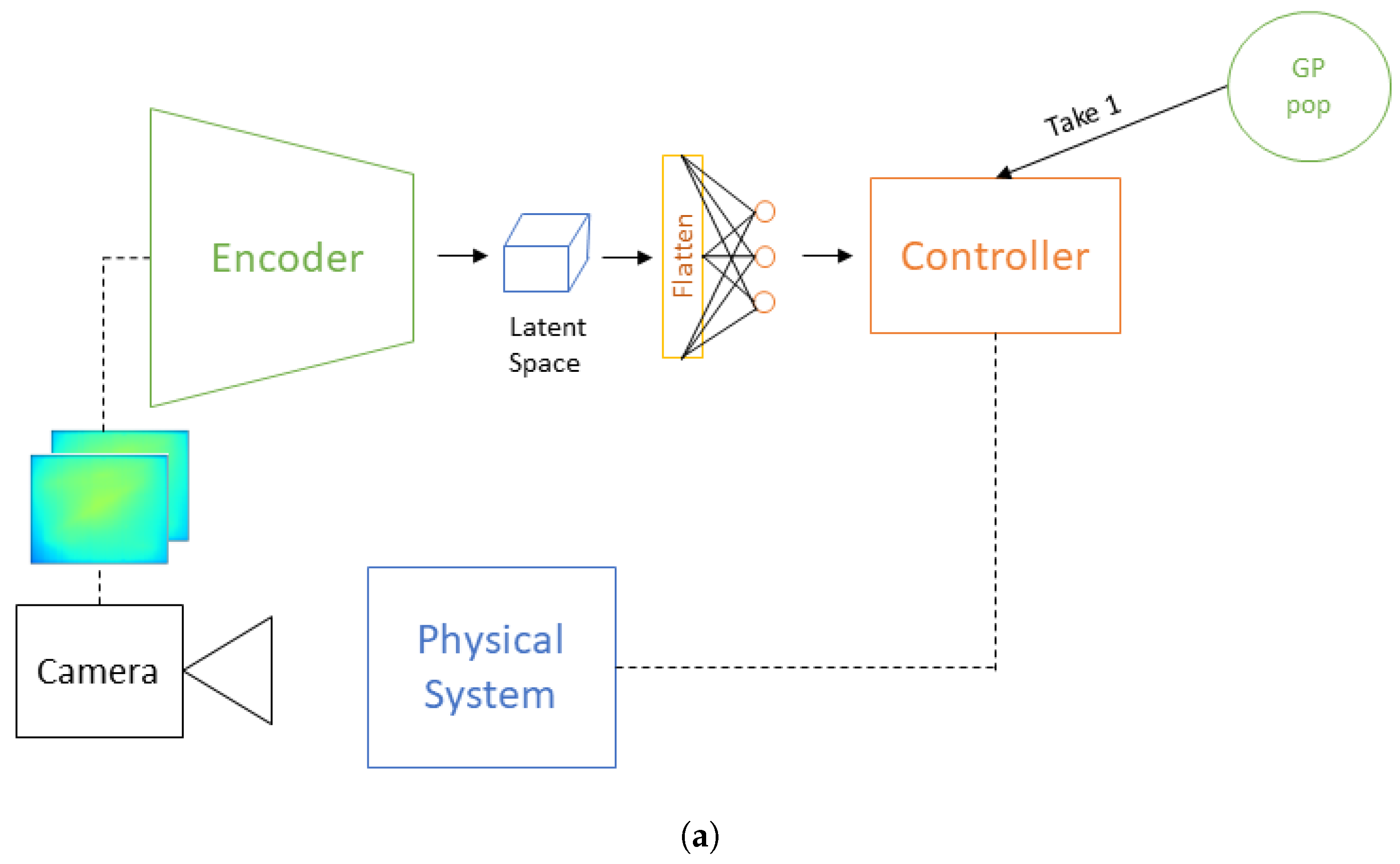
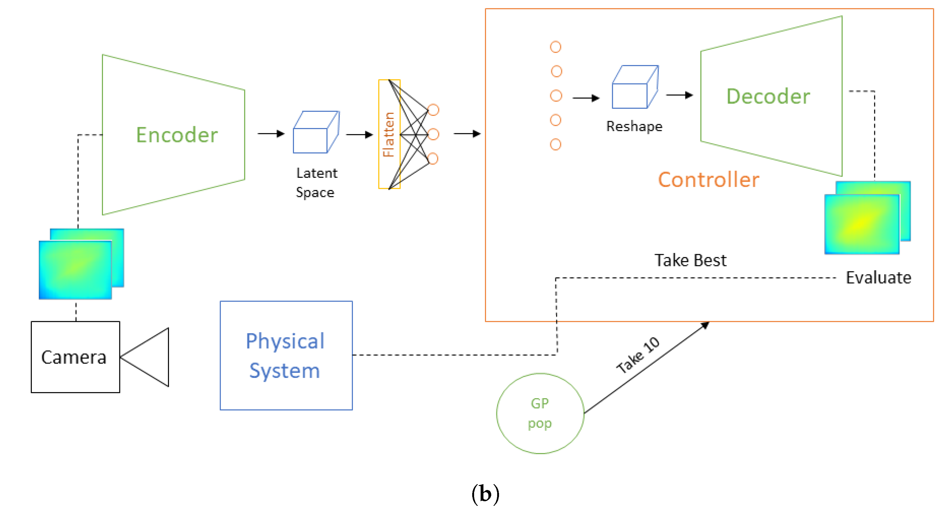
2.4. Control Policy Generation Using Genetic Programming
Control Model Architecture
3. Results
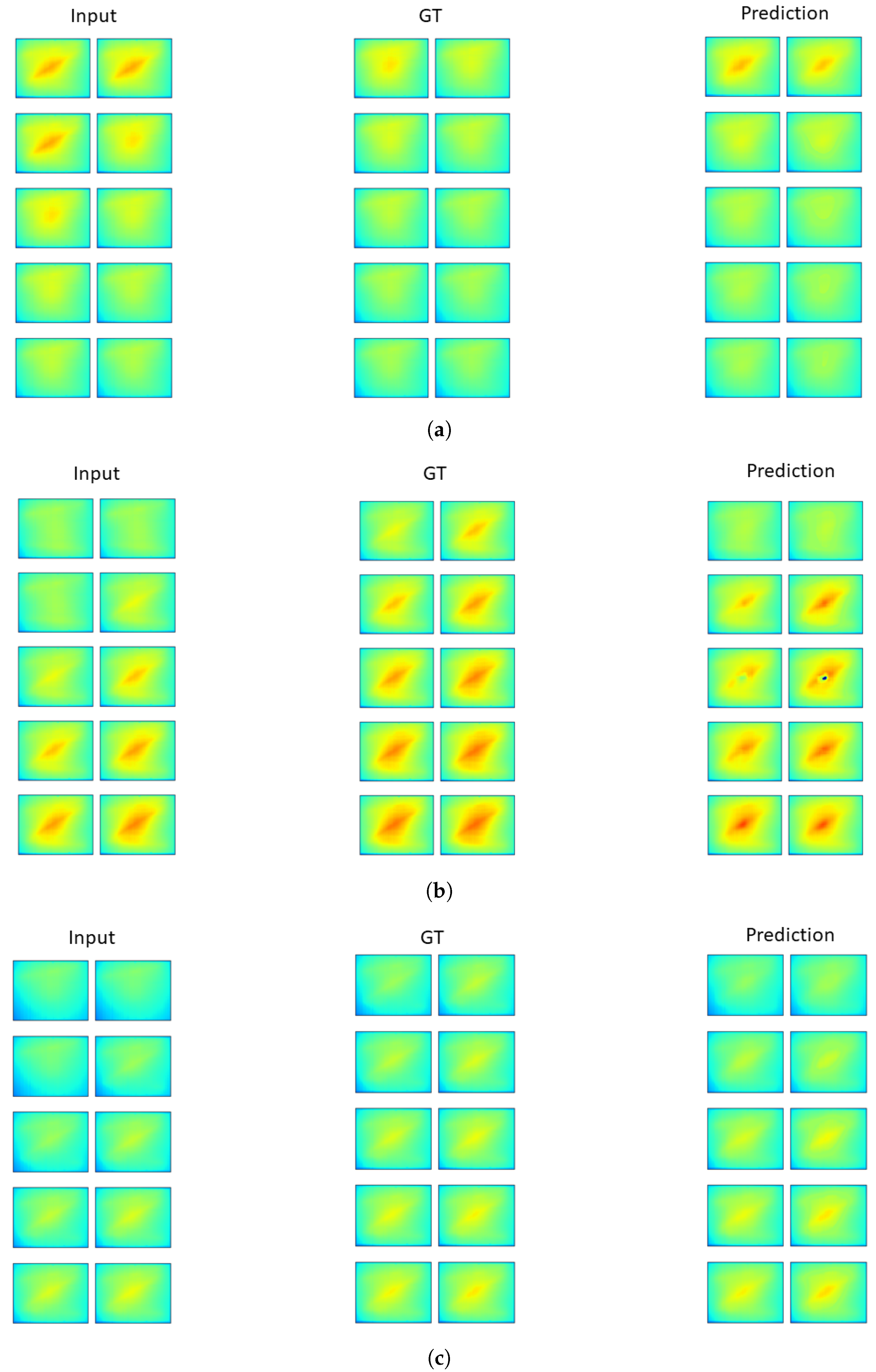
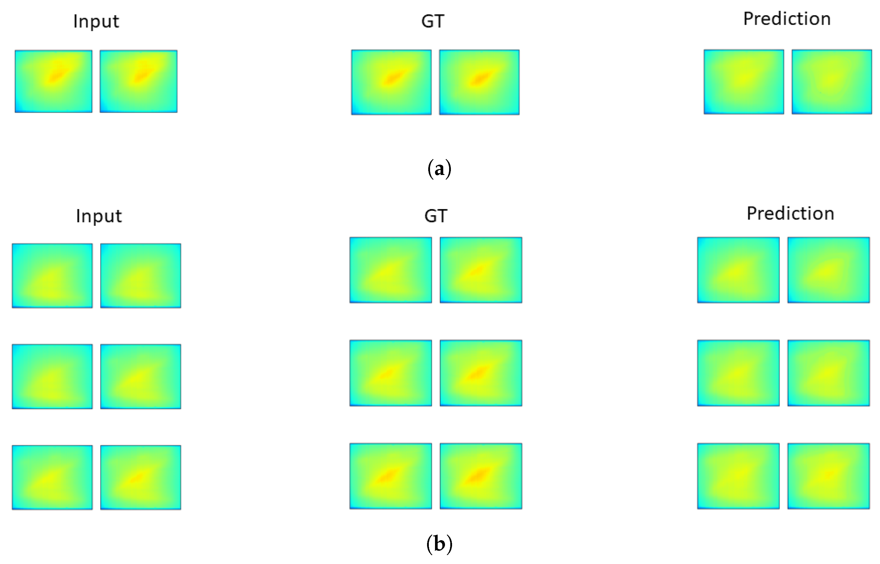
3.1. Testing Digital Twin as a Predictive Model
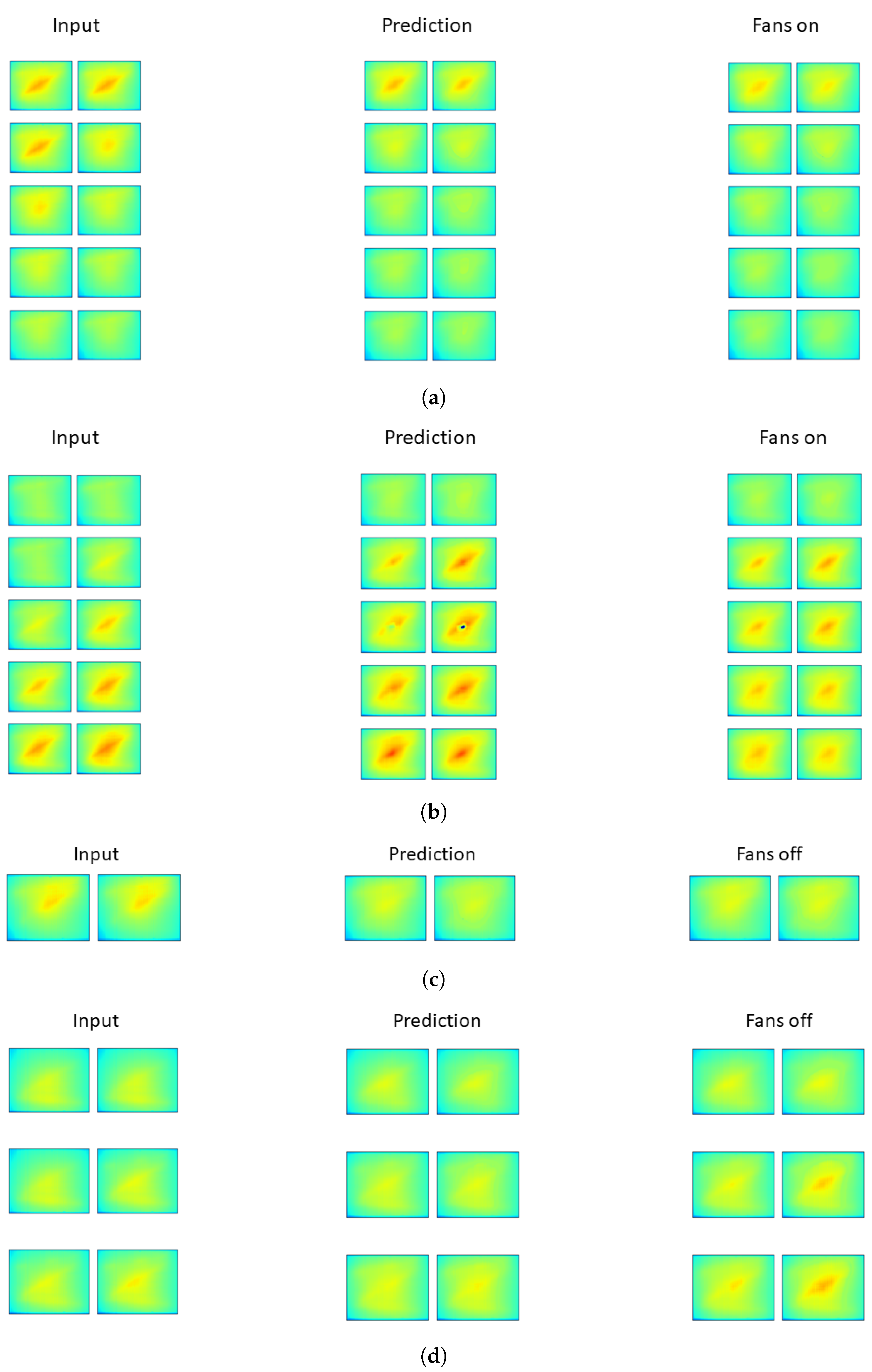
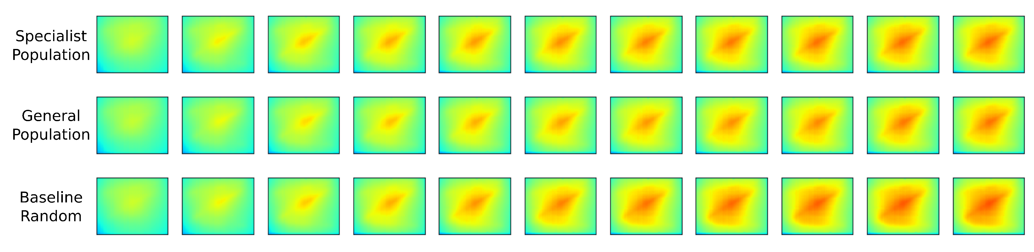
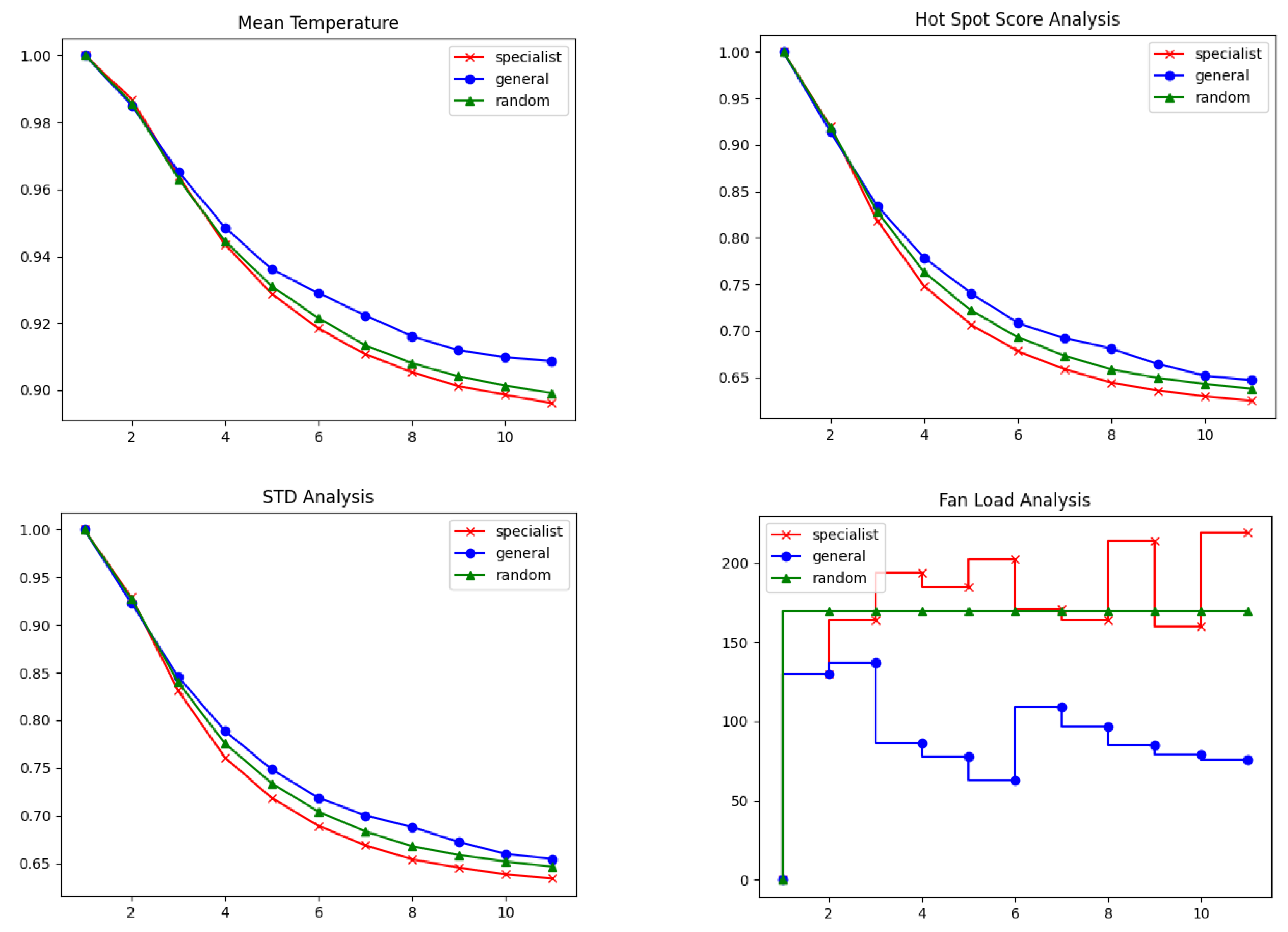
3.2. Model Predictive Controller Performance
4. Discussions
5. Conclusions
Author Contributions
Funding
Data Availability Statement
Acknowledgments
Conflicts of Interest
Nomenclature
| ARIMA | Autoregressive moving average model |
| CNN | Convolutional neural network |
| ConvLSTM | Convolutional Long Short-Term Memory |
| DT | Digital twin |
| FSP | Fixed set-point |
| GA | Genetic algorithm |
| GP | Genetic programming |
| HDF | Hierarchical data format |
| HVAC | Heating, ventilation and air conditioning |
| LIDAR | Light detection and ranging |
| MAE | Mean absolute error |
| MAPE | Mean absolute percentage error |
| MSE | Mean squared error |
| MPC | Model predictive control |
| NARIMAX | Nonlinear Autoregressive moving average model with exogenous inputs |
| NN | Neural networks |
| PID | Proportional–integral–derivative controller |
| PSO | Particle swarm optimization |
| RNN | Recurrent neural network |
| ReLU | Rectified linear unit |
| STD | Standard deviation |
Appendix A. Background of the Deployed Digital Twin Model
Appendix B. GP Controller Hyperparameters and Operators

| Parameter/Operator | Value/Policy | Argument |
|---|---|---|
| Mutation Probability | 0.05 | To prevent the loss of good solutions while maintaining diversity in the gene pool. |
| Crossover Probability | 0.85 | To avoid unnecessary population shrinkage and prevent excessively fast convergence. |
| Tree Depth | 15–25 | Shallow trees would only utilize a small portion of the inputs and would be insufficient for generating sophisticated control laws. Deeper trees, however, require longer computational times for evaluation. |
| Selection Strategy | Tournament selection | This strategy is widely used and has shown acceptable results. According to [41], all selection strategies can generate satisfactory outcomes, except for roulette, which is not suitable for minimization tasks. |
| Tournament Size | 2 | A smaller tournament size preserves greater variety in the gene pool. |
| Population Size | 300 | A larger initial population ensures a more diverse gene pool. However, it also leads to longer training times. To capitalize on the processing power of our GPU unit, we explore a broader set of initial candidates. |
| Output Filter | Sigmoid | The outputs of the trees are scaled to values between 0 and 1 using the sigmoid function. |
- Linear operations—summation, addition, subtraction, multiplication and negation;
- Trigonometric operations—sine and cosine—these operators are used to scale the floating point numbers in the tree. This prevents an “explosion” of the values in either direction (positive or negative), resulting in only two possible modes of operation for the fans—either 0% or 100% load;
- Regrouping operations—create a 3D vector from three values—this is a hard-coded function for the output of the tree, which should result in a 3D vector with one value for the duty cycle of each fan.
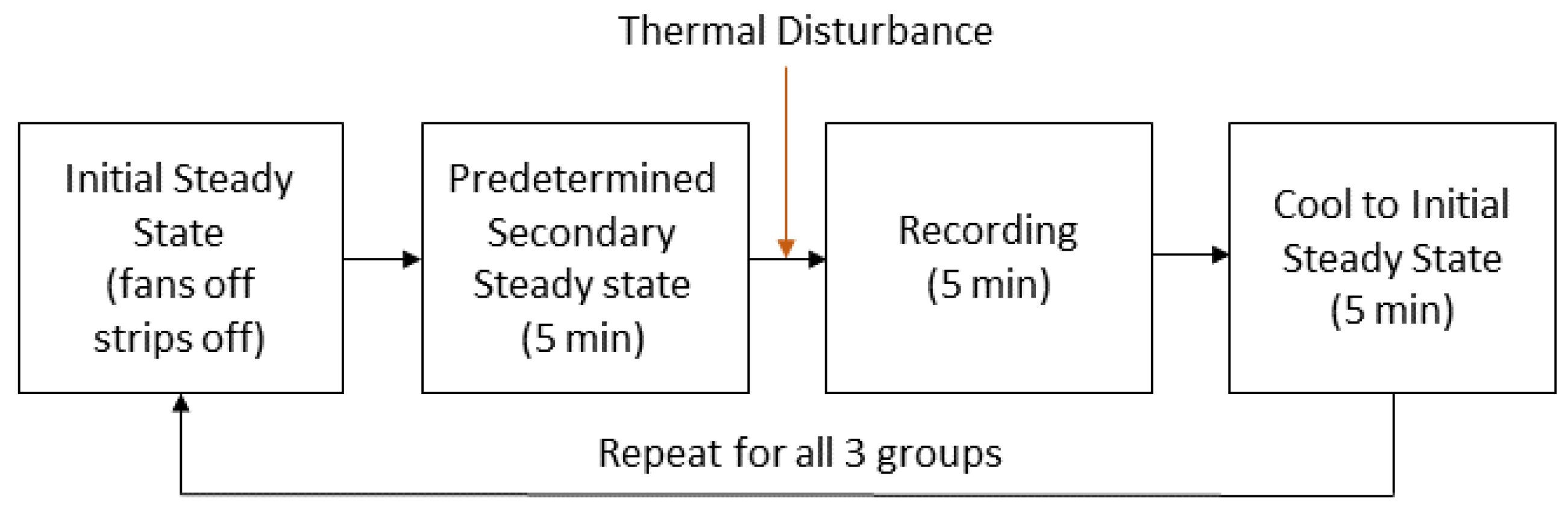
Appendix C. MPC Experiment Design


- 1.
- Cooling to the initial state: All experiments begin from the same starting point by cooling the system to the initial state. This step ensures consistency across experiments.
- 2.
- Recreating a predetermined steady state: To simulate the control of a dynamic system and replicate a realistic scenario, the system is preheated to a predetermined secondary steady state. This step further enhances the reliability of the evaluation.
- 3.
- Fixed experiment duration: Each experiment is conducted for a fixed duration of 5 min, with a frame captured every 30 s. This extended monitoring period allows for a comprehensive observation of the evolution of the temperature field.
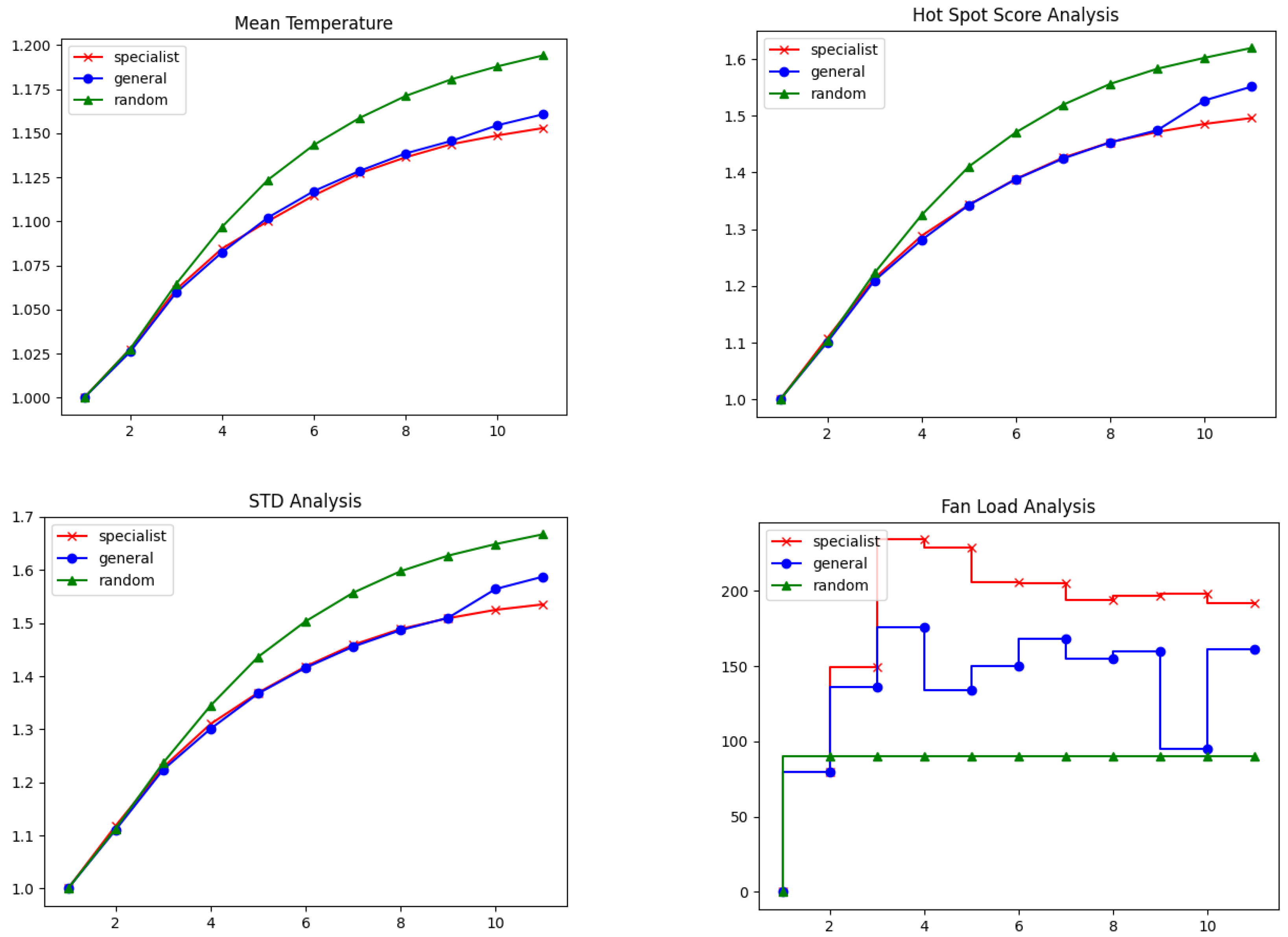
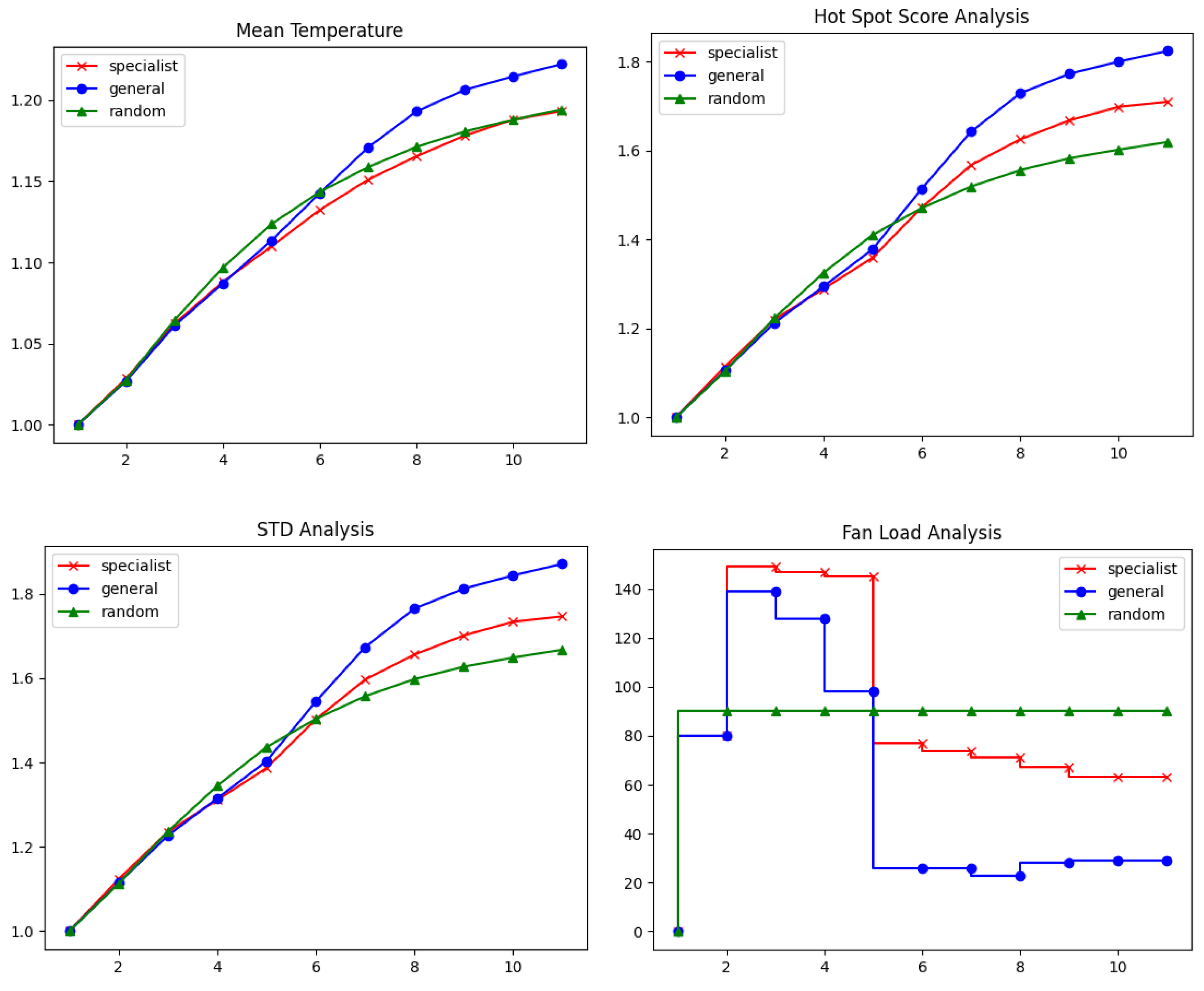
- High heat loading: the load on the heating strips was suddenly increased from [50%, 25% and 0%] to [75%, 100% and 75%], while the fans were open at [20%, 40% and 20%]. The benchmark control law resulted in a fan setting for the cooling experiment of [70%, 0% and 20%] after the set point change.
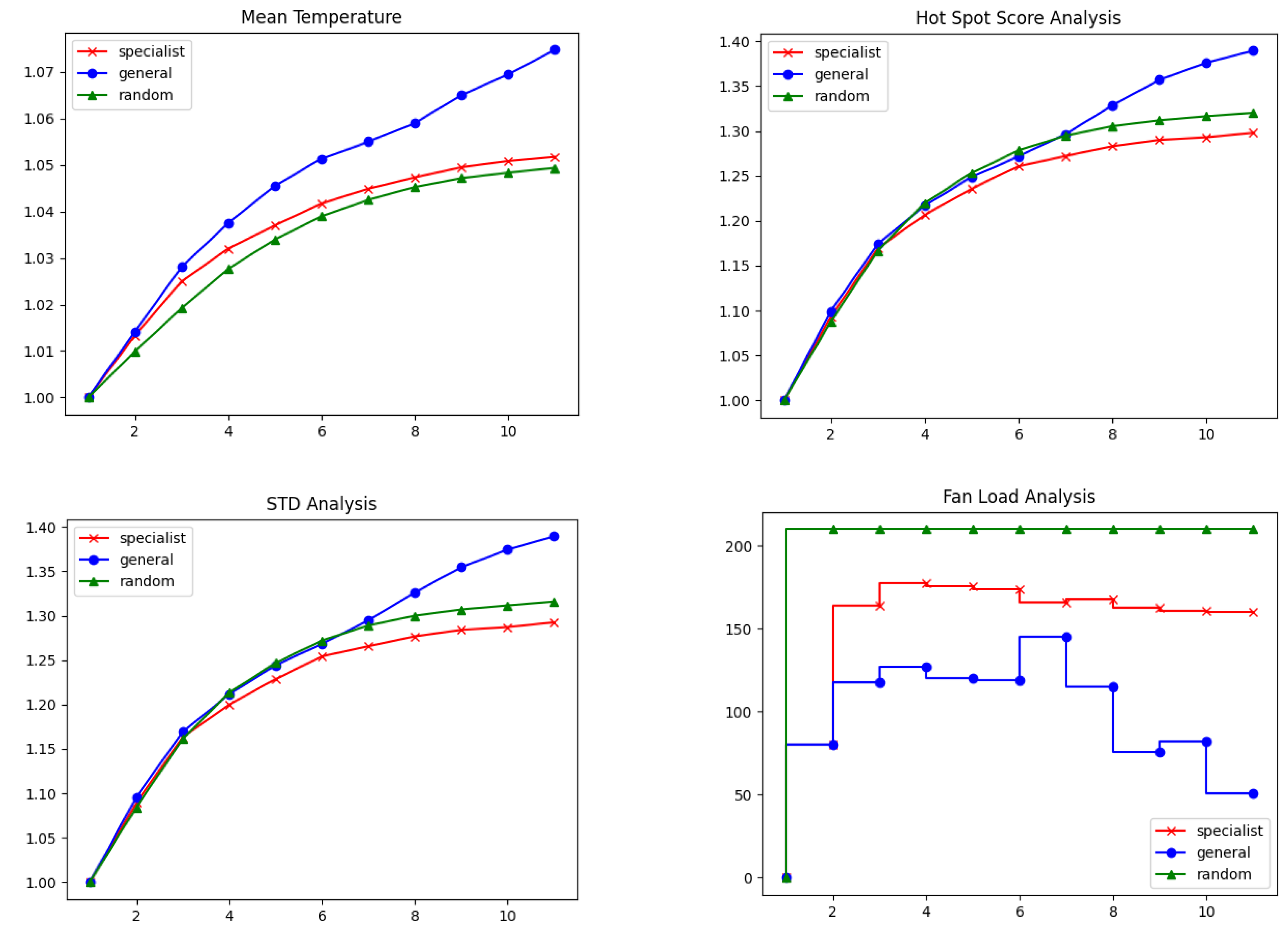
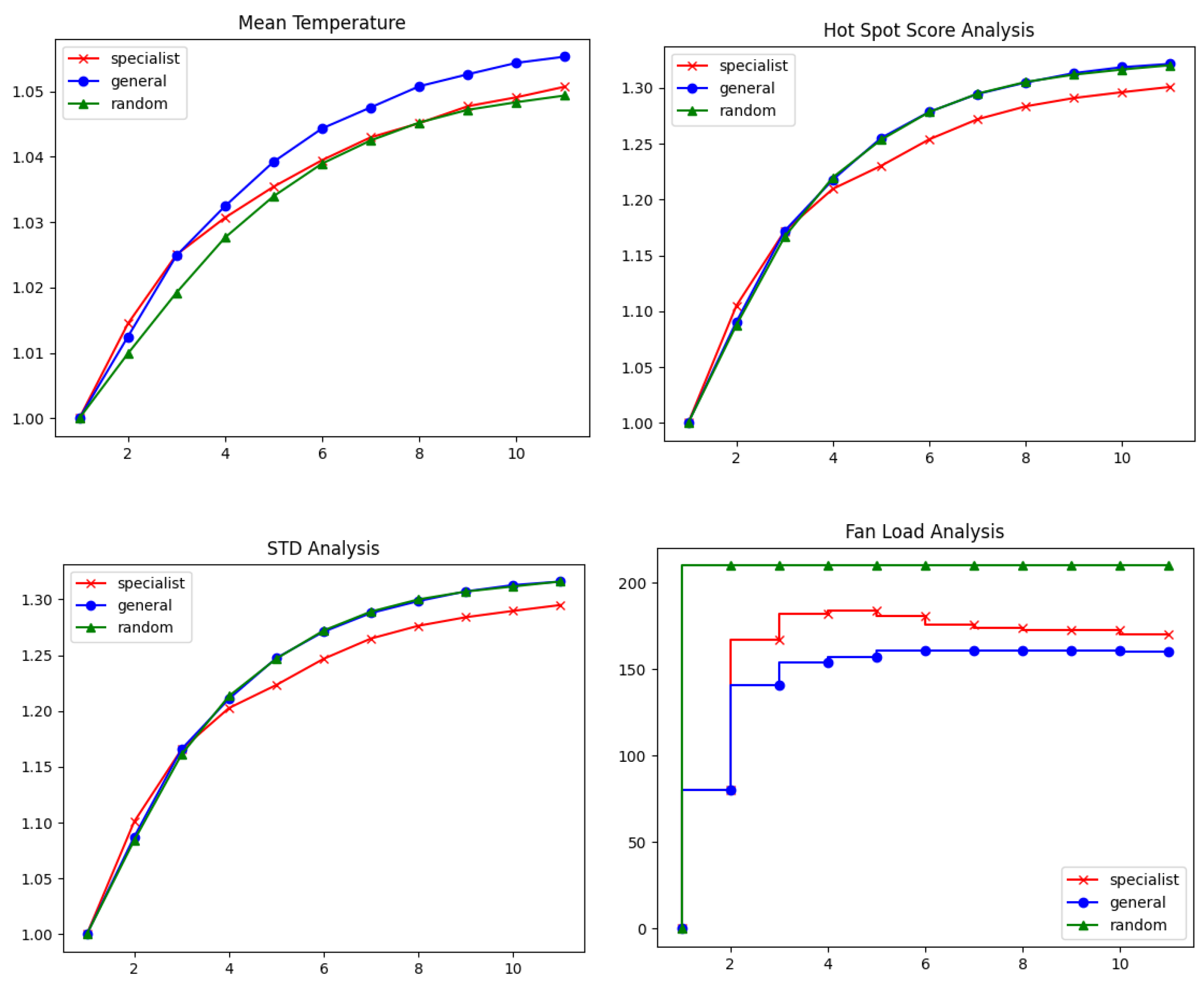
- Medium heat loading: the heating strip loads were suddenly raised from [25%, 0% and 50%] to [25%, 50% and 70%], while the fans were open at [30%, 20% and 30%] during the second steady state. In this situation, the benchmark control law adjusted the fan settings to [30%, 80% and 100%].
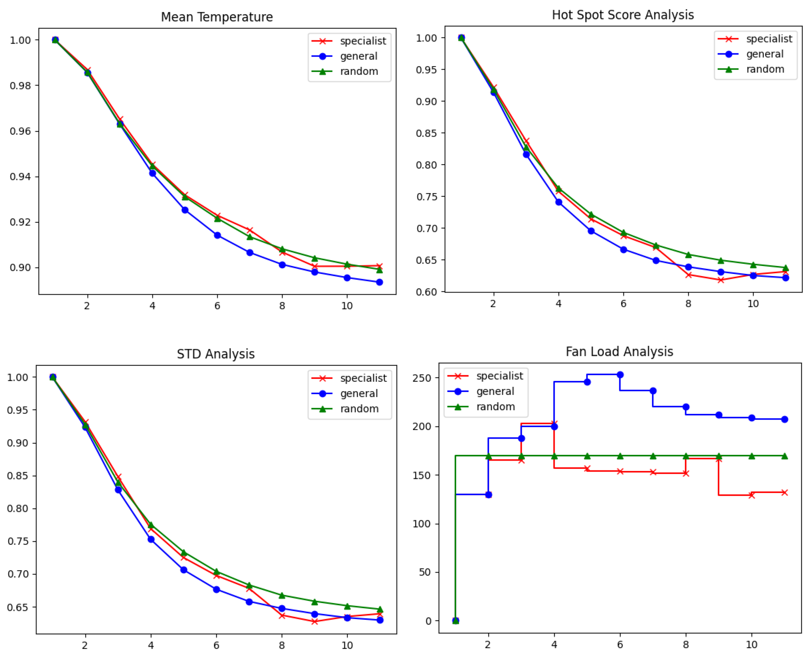
- Low heat loading: the thermal load was abruptly reduced from [75%, 75% and 50%] to [0%, 25% and 25%], while the fans were open at [50%, 80% and 0%]. In this case, the benchmark controller set the fan settings to [80%, 50% and 40%].
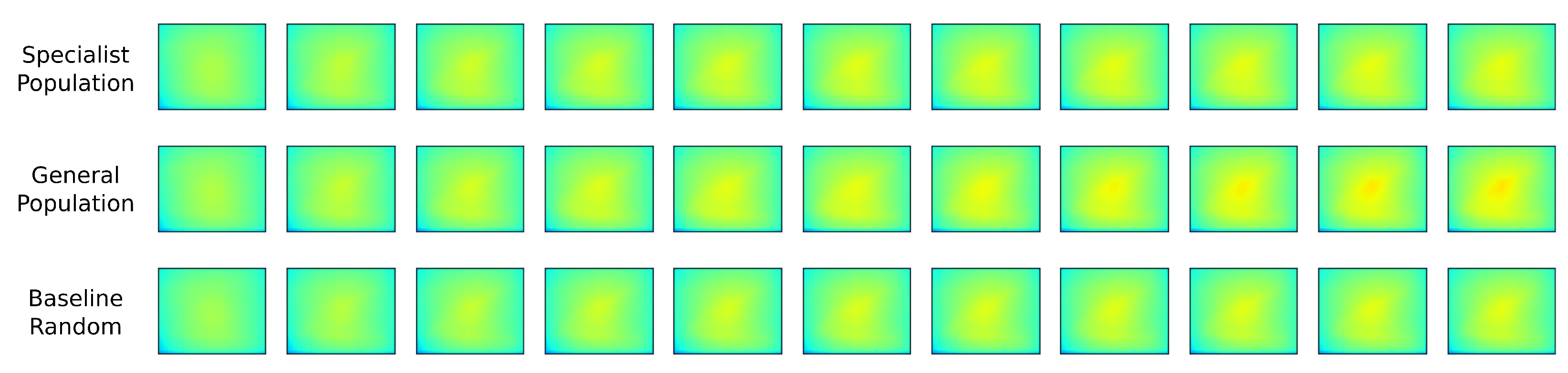
Appendix D. Single Individual Tests
Appendix D.1. High Load Test Case

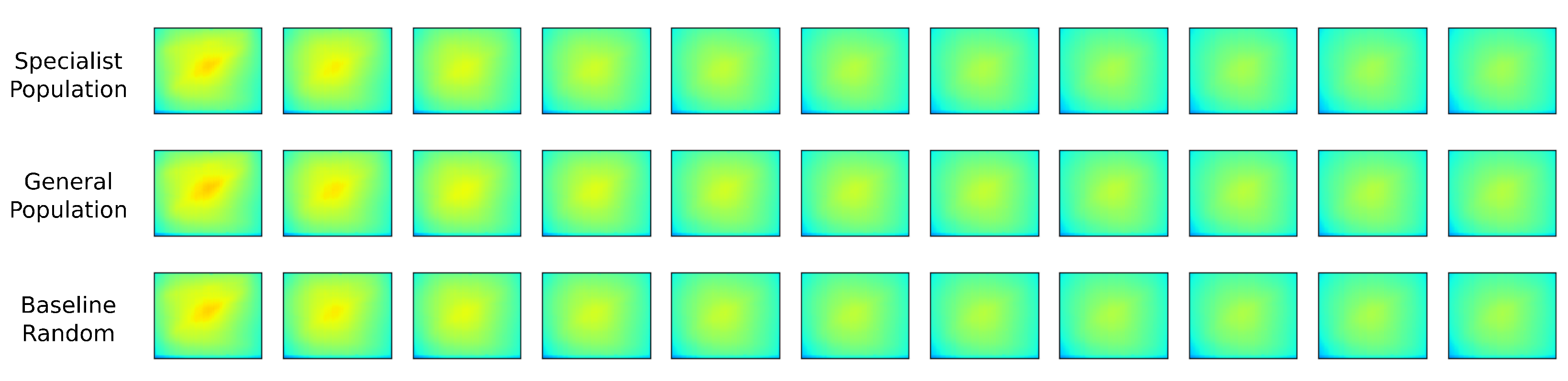
Appendix D.2. Medium Load Test Case

Appendix D.3. Low Load Test Case

References
- Marusak, P.M. Numerically Efficient Fuzzy MPC Algorithm with Advanced Generation of Prediction—Application to a Chemical Reactor. Algorithms 2020, 13, 143. [Google Scholar] [CrossRef]
- Nebeluk, R.; Ławryńczuk, M. Tuning of Multivariable Model Predictive Control for Industrial Tasks. Algorithms 2021, 14, 10. [Google Scholar] [CrossRef]
- Domański, P.D. Performance Assessment of Predictive Control—A Survey. Algorithms 2020, 13, 97. [Google Scholar] [CrossRef] [Green Version]
- Wright, L.; Davidson, S. How to tell the difference between a model and a digital twin. Adv. Model. Simul. Eng. Sci. 2020, 7, 13. [Google Scholar] [CrossRef]
- Sun, C.; Shi, V.G. PhysiNet: A combination of physics-based model and neural network model for digital twins. Int. J. Intell. Syst. 2022, 37, 5443–5456. [Google Scholar] [CrossRef]
- Shi, X.; Chen, Z.; Wang, H.; Yeung, D.Y.; Wong, W.K.; Woo, W.C. Convolutional LSTM network: A machine learning approach for precipitation nowcasting. In Proceedings of the Advances in Neural Information Processing Systems 28 (NIPS 2015), Montreal, QC, Canada, 7–12 December 2015; pp. 1–9. [Google Scholar]
- Liu, C.; Atkeson, C.G. Standing balance control using a trajectory library. In Proceedings of the 2009 IEEE/RSJ International Conference on Intelligent Robots and Systems, St. Louis, MO, USA, 10–15 October 2009; pp. 3031–3036. [Google Scholar] [CrossRef] [Green Version]
- Koller, T.; Berkenkamp, F.; Turchetta, M.; Krause, A. Learning-Based Model Predictive Control for Safe Exploration. In Proceedings of the 2018 IEEE Conference on Decision and Control (CDC), Miami Beach, FL, USA, 17–19 December 2018; pp. 6059–6066. [Google Scholar] [CrossRef] [Green Version]
- Tavakoli, M.; Shokridehaki, F.; Marzband, M.; Godina, R.; Pouresmaeil, E. A two stage hierarchical control approach for the optimal energy management in commercial building microgrids based on local wind power and PEVs. Sustain. Cities Soc. 2018, 41, 332–340. [Google Scholar] [CrossRef]
- Maddalena, E.T.; Müller, S.A.; dos Santos, R.M.; Salzmann, C.; Jones, C.N. Experimental data-driven model predictive control of a hospital HVAC system during regular use. Energy Build. 2022, 271, 112316. [Google Scholar] [CrossRef]
- McKinnon, C.D.; Schoellig, A.P. Learn Fast, Forget Slow: Safe Predictive Learning Control for Systems with Unknown and Changing Dynamics Performing Repetitive Tasks. IEEE Robot. Autom. Lett. 2019, 4, 2180–2187. [Google Scholar] [CrossRef] [Green Version]
- Wang, H.; Chen, Y.; Kang, J.; Ding, Z.; Zhu, H. An XGBoost-Based predictive control strategy for HVAC systems in providing day-ahead demand response. Build. Environ. 2023, 238, 110350. [Google Scholar] [CrossRef]
- Ay, M.; Stemmler, S.; Schwenzer, M.; Abel, D.; Bergs, T. Model Predictive Control in Milling based on Support Vector Machines. IFAC-PapersOnLine 2019, 52, 1797–1802. [Google Scholar] [CrossRef]
- Piche, S.; Sayyar-Rodsari, B.; Johnson, D.; Gerules, M. Nonlinear model predictive control using neural networks. IEEE Control. Syst. Mag. 2000, 20, 53–62. [Google Scholar] [CrossRef]
- Mu, J.; Rees, D. Approximate model predictive control for gas turbine engines. In Proceedings of the 2004 American Control Conference, Boston, MA, USA, 30 June–2 July 2004; Volume 6, pp. 5704–5709. [Google Scholar] [CrossRef]
- Afram, A.; Janabi-Sharifi, F.; Fung, A.S.; Raahemifar, K. Artificial neural network (ANN) based model predictive control (MPC) and optimization of HVAC systems: A state of the art review and case study of a residential HVAC system. Energy Build. 2017, 141, 96–113. [Google Scholar] [CrossRef]
- Li, S.; Jiang, P.; Han, K. RBF Neural Network based Model Predictive Control Algorithm and its Application to a CSTR Process. In Proceedings of the 2019 Chinese Control Conference (CCC), Guangzhou, China, 27–30 July 2019; pp. 2948–2952. [Google Scholar] [CrossRef]
- Maddalena, E.; Moraes, C.D.S.; Waltrich, G.; Jones, C. A Neural Network Architecture to Learn Explicit MPC Controllers from Data. IFAC-PapersOnLine 2020, 53, 11362–11367. [Google Scholar] [CrossRef]
- Nubert, J.; Köhler, J.; Berenz, V.; Allgöwer, F.; Trimpe, S. Safe and Fast Tracking on a Robot Manipulator: Robust MPC and Neural Network Control. IEEE Robot. Autom. Lett. 2020, 5, 3050–3057. [Google Scholar] [CrossRef] [Green Version]
- Shin, Y.; Smith, R.; Hwang, S. Development of model predictive control system using an artificial neural network: A case study with a distillation column. J. Clean. Prod. 2020, 277, 124124. [Google Scholar] [CrossRef]
- Núñez, F.; Langarica, S.; Díaz, P.; Torres, M.; Salas, J.C. Neural Network-Based Model Predictive Control of a Paste Thickener Over an Industrial Internet Platform. IEEE Trans. Ind. Inform. 2020, 16, 2859–2867. [Google Scholar] [CrossRef]
- Pan, Y.; Wang, J. Model predictive control of unknown nonlinear dynamical systems based on recurrent neural networks. IEEE Trans. Ind. Electron. 2012, 59, 3089–3101. [Google Scholar] [CrossRef]
- Pon Kumar, S.S.; Tulsyan, A.; Gopaluni, B.; Loewen, P. A Deep Learning Architecture for Predictive Control. IFAC-PapersOnLine 2018, 51, 512–517. [Google Scholar] [CrossRef]
- Shahnazari, H.; Mhaskar, P.; House, J.M.; Salsbury, T.I. Modeling and fault diagnosis design for HVAC systems using recurrent neural networks. Comput. Chem. Eng. 2019, 126, 189–203. [Google Scholar] [CrossRef]
- Wu, Z.; Tran, A.; Rincon, D.; Christofides, P.D. Machine learning-based predictive control of nonlinear processes. Part I: Theory. AIChE J. 2019, 65, e16729. [Google Scholar] [CrossRef]
- Wu, Z.; Rincon, D.; Christofides, P.D. Real-Time Adaptive Machine-Learning-Based Predictive Control of Nonlinear Processes. Ind. Eng. Chem. Res. 2020, 59, 2275–2290. [Google Scholar] [CrossRef]
- Huang, K.; Wei, K.; Li, F.; Yang, C.; Gui, W. LSTM-MPC: A Deep Learning Based Predictive Control Method for Multimode Process Control. IEEE Trans. Ind. Electron. 2022, 70, 11544–11554. [Google Scholar] [CrossRef]
- Zarzycki, K.; Ławryńczuk, M. Advanced predictive control for GRU and LSTM networks. Inf. Sci. 2022, 616, 229–254. [Google Scholar] [CrossRef]
- Zheng, Y.; Zhao, T.; Wang, X.; Wu, Z. Online learning-based predictive control of crystallization processes under batch-to-batch parametric drift. AIChE J. 2022, 68, e17815. [Google Scholar] [CrossRef]
- Cho, M.; Ban, J.; Seo, M.; Kim, S.W. Neural network MPC for heating section of annealing furnace. Expert Syst. Appl. 2023, 223, 119869. [Google Scholar] [CrossRef]
- Jung, M.; da Costa Mendes, P.R.; Önnheim, M.; Gustavsson, E. Model Predictive Control when utilizing LSTM as dynamic models. Eng. Appl. Artif. Intell. 2023, 123, 106226. [Google Scholar] [CrossRef]
- Meng, J.; Li, C.; Tao, J.; Li, Y.; Tong, Y.; Wang, Y.; Zhang, L.; Dong, Y.; Du, J. RNN-LSTM-Based Model Predictive Control for a Corn-to-Sugar Process. Processes 2023, 11, 1080. [Google Scholar] [CrossRef]
- Achirei, S.D.; Mocanu, R.; Popovici, A.T.; Dosoftei, C.C. Model-Predictive Control for Omnidirectional Mobile Robots in Logistic Environments Based on Object Detection Using CNNs. Sensors 2023, 23, 4992. [Google Scholar] [CrossRef] [PubMed]
- Sands, T. Comparison and Interpretation Methods for Predictive Control of Mechanics. Algorithms 2019, 12, 232. [Google Scholar] [CrossRef] [Green Version]
- Rosolia, U.; Zhang, X.; Borrelli, F. Data-Driven Predictive Control for Autonomous Systems. Annu. Rev. Control. Robot. Auton. Syst. 2018, 1, 259–286. [Google Scholar] [CrossRef]
- Rawlings, J.B.; Maravelias, C.T. Bringing new technologies and approaches to the operation and control of chemical process systems. AIChE J. 2019, 65, e16615. [Google Scholar] [CrossRef]
- Schwenzer, M.; Ay, M.; Bergs, T.; Abel, D. Review on model predictive control: An engineering perspective. Int. J. Adv. Manuf. Technol. 2021, 117, 1327–1349. [Google Scholar] [CrossRef]
- Schweidtmann, A.M.; Esche, E.; Fischer, A.; Kloft, M.; Repke, J.U.; Sager, S.; Mitsos, A. Machine Learning in Chemical Engineering: A Perspective. Chemie-Ingenieur-Technik 2021, 93, 2029–2039. [Google Scholar] [CrossRef]
- De Myttenaere, A.; Golden, B.; Le Grand, B.; Rossi, F. Mean absolute percentage error for regression models. Neurocomputing 2016, 192, 38–48. [Google Scholar] [CrossRef] [Green Version]
- Nazmul Siddique, H. Intelligent Control: A Hybrid Approach Based on Fuzzy Logic, Neural Networks and Genetic Algorithms; Springer: Cham, Switzerland, 2013. [Google Scholar]
- Ahvanooey, M.T.; Li, Q.; Wu, M.; Wang, S. A Survey of Genetic Programming and Its Applications. KSII Trans. Internet Inf. Syst. 2019, 13, 1765–1794. [Google Scholar]
- Zheng, C.; Eskandari, M.; Li, M.; Sun, Z. GA-Reinforced Deep Neural Network for Net Electric Load Forecasting in Microgrids with Renewable Energy Resources for Scheduling Battery Energy Storage Systems. Algorithms 2022, 15, 338. [Google Scholar] [CrossRef]
- Koza, J.R.; Keane, M.A.; Yu, J.; Bennett, F.H.; Mydlowec, W. Automatic creation of human-competitive programs and controllers by means of genetic programming. Genet. Program. Evolvable Mach. 2000, 1, 121–164. [Google Scholar] [CrossRef]
- Grosman, B.; Lewin, D.R. Automated nonlinear model predictive control using genetic programming. Comput. Chem. Eng. 2002, 26, 631–640. [Google Scholar] [CrossRef]
- Vyas, R.; Goel, P.; Tambe, S.S. Genetic programming applications in chemical sciences and engineering. In Handbook of Genetic Programming Applications; Springer: Cham, Switzerland, 2015; pp. 99–140. [Google Scholar]
- Lotter, W.; Kreiman, G.; Cox, D. Deep predictive coding networks for video prediction and unsupervised learning. arXiv 2016, arXiv:1605.08104. [Google Scholar]
- Hosseini, M.; Maida, A.S.; Hosseini, M.; Raju, G. Inception-inspired lstm for next-frame video prediction. arXiv 2019, arXiv:1909.05622. [Google Scholar]
- Plaster, B.; Kumar, G. Data-Driven Predictive Modeling of Neuronal Dynamics Using Long Short-Term Memory. Algorithms 2019, 12, 203. [Google Scholar] [CrossRef] [Green Version]
- Desai, P.; Sujatha, C.; Chakraborty, S.; Ansuman, S.; Bhandari, S.; Kardiguddi, S. Next frame prediction using ConvLSTM. J. Phys. Conf. Ser. 2022, 2161, 012024. [Google Scholar] [CrossRef]
- Hong, S.; Kim, S.; Joh, M.; Song, S.K. Psique: Next sequence prediction of satellite images using a convolutional sequence-to-sequence network. arXiv 2017, arXiv:1711.10644. [Google Scholar]
- Tang, M.; Liu, Y.; Durlofsky, L.J. A deep-learning-based surrogate model for data assimilation in dynamic subsurface flow problems. J. Comput. Phys. 2020, 413, 109456. [Google Scholar] [CrossRef] [Green Version]
- Kakka, P.R. Sequence to sequence AE-ConvLSTM network for modelling the dynamics of PDE systems. arXiv 2022, arXiv:2208.07315. [Google Scholar]
- Mukherjee, S.; Ghosh, S.; Ghosh, S.; Kumar, P.; Roy, P.P. Predicting video-frames using encoder-convlstm combination. In Proceedings of the ICASSP 2019—2019 IEEE International Conference on Acoustics, Speech and Signal Processing (ICASSP), Brighton, UK, 12–17 May 2019; pp. 2027–2031. [Google Scholar]


| Duration in Frames | Number of Experiments |
|---|---|
| 8 | 32 |
| 9 | 103 |
| 10 | 85 |
| 11 | 48 |
| 12 | 35 |
| 13 | 16 |
| 14 | 4 |
Disclaimer/Publisher’s Note: The statements, opinions and data contained in all publications are solely those of the individual author(s) and contributor(s) and not of MDPI and/or the editor(s). MDPI and/or the editor(s) disclaim responsibility for any injury to people or property resulting from any ideas, methods, instructions or products referred to in the content. |
© 2023 by the authors. Licensee MDPI, Basel, Switzerland. This article is an open access article distributed under the terms and conditions of the Creative Commons Attribution (CC BY) license (https://creativecommons.org/licenses/by/4.0/).
Share and Cite
Ates, C.; Bicat, D.; Yankov, R.; Arweiler, J.; Koch, R.; Bauer, H.-J. Model Predictive Evolutionary Temperature Control via Neural-Network-Based Digital Twins. Algorithms 2023, 16, 387. https://doi.org/10.3390/a16080387
Ates C, Bicat D, Yankov R, Arweiler J, Koch R, Bauer H-J. Model Predictive Evolutionary Temperature Control via Neural-Network-Based Digital Twins. Algorithms. 2023; 16(8):387. https://doi.org/10.3390/a16080387
Chicago/Turabian StyleAtes, Cihan, Dogan Bicat, Radoslav Yankov, Joel Arweiler, Rainer Koch, and Hans-Jörg Bauer. 2023. "Model Predictive Evolutionary Temperature Control via Neural-Network-Based Digital Twins" Algorithms 16, no. 8: 387. https://doi.org/10.3390/a16080387