1. Introduction
One of the most fundamental pillars of modern life is telecommunication in general, and wireless telecommunication networks in particular. These serve literally billions of requests every week, and not only for phones, but also devices from the Internet of Things (IoT). In this paper, we refer to all these different units as users.
The first wireless networks were constructed around 1970, and were envisaged to be built from small
cells, each cell served by one
base station (
BS for short), so the network was decomposed into smaller parts that served the users independently from each other. (At this time the users were bulky
mobile phones; see, for example [
1]). While this idea is simple, the design is afflicted by the well-known
cell-edge problem: users located in the overlapping area of two cells suffer from strong interference from the neighboring BSs. This problem has created a considerable challenge for service providers.
In the current coordinated multipoint (CoMP) transmission technology, several (typically physically close) base stations are organized, permanently or dynamically, into one cell, and the BSs in the same cell jointly serve all the users in this cell. The goal of this approach is again to decompose a large-scale network into smaller parts: the constructed clusters (again called cells) have less engineering complexity than the original network and they can operate in parallel.
Currently, considering the enormous number of base stations and users, and in spite of the multi-cell approach, the cell-edge problem stubbornly remains with us (see [
2]). For 5G networks, the cell-edge problem can become even more pronounced because more users fall into the cell-edge area as the size of each cell shrinks (see [
3]).
Mathematically speaking, minimizing the cell-edge problem belongs to the family of clustering problems: given a set of (not necessarily) homogeneous objects, we want to divide the objects into pairwise disjoint classes while optimizing some “measure” of the resulting set of classes.
Myriads of theoretical and practical problems belong to the clustering framework. They come from classical combinatorial optimization problems to printed circuit board designs, from VLSI CAD applications to distributing tasks among processors for supercomputing processes, and from pattern recognition to computer vision problems and image retrieval. The computational complexity of these problems varies from easy to very hard. For example, the minimum number of edges whose deletion places two predefined vertices into separate components in a simple graph (
minimum cut problem [
4]) can be computed in polynomial time. The situation changes dramatically if we want to separate three predefined vertices (
the multiway cut problem). In the general case, this generalization of the problem was shown to be NP-hard [
5], while the problem becomes fixed parameter tractable if the input is restricted to planar graphs [
5,
6].
Probably, the very first engineering problem of a clustering nature was the following: we want to place a complicated electronic design on printed circuit boards, where each board can contain at most
k components and where the electronic connections among the boards are expensive compared to connections inside a board ([
7], see also [
8]). It can be seen that in such a real-world problem, an upper bound on the possible size of the clusters is given too. While the notion of NP-completeness was being developed at the time, the authors correctly placed the problem into the NP-hard class.
The majority of the clustering problems are NP-hard, so there is no chance to solve them exactly. Sometimes there are known performance guarantees on the solution; for example, in [
5], there is a polynomial time algorithm with a
approximation ratio for the multiway-cut problem, while in [
9], a polynomial time
approximation algorithm was developed for the same problem.
The interference minimization problem in wireless networks is a known NP-hard problem, and so far a constant factor approximation algorithm has not been found. In the literature, there are several approaches to solve this problem, see [
1,
10,
11,
12,
13,
14]. Because of the intractability of the problem, all of these approaches are heuristic in nature. In practice, these methods still do not satisfactorily solve the cell-edge problem [
2].
Essentially, all of these method use one of the general clustering methods: the
kernel k-means or the
spectral clustering method. The former method was developed in [
15,
16]. However, as was proved in [
17], the two approaches are essentially equivalent with each other (for a survey on these methods, see [
18]). Consequently, we compare our algorithm to the spectral clustering method (as it is used in [
3]). This approach attacks this clustering problem as an undivided one, partitioning the base stations and users simultaneously. However, the two sets of agents typically have different cardinalities, and their elements have very different functions and properties in the network.
In this paper, we propose a simple and fast clustering algorithm to deal with the cell-edge problem. (An earlier version of this algorithm was reported in [
19]). Our algorithm runs significantly faster than the spectral clustering method, and simulations on synthetic instances indicate that our proposed method typically provides higher quality solutions than the application of the spectral clustering method in [
3]. In contrast with the spectral clustering methods, our proposed heuristic method is deterministic.
We divide the interference minimization problem into three subproblems. In the first phase, a new, so-called dot-product similarity measure is introduced on pairs of base stations. This similarity measure is based on the dynamically changing signal strengths between the users and the base stations. The two subsequent phases are two clustering problems. The second phase partitions the base stations into clusters, and the third phase assigns the users to base station clusters. The solution to the whole problem is given as a pairing between the base station clusters and user clusters.
Our reason for this handling is the following observation: the roles of the base stations and the users are different, and so they require different considerations. We emphasize this asymmetry with our notation system as well. The clusters of the entire system appear as pairs of clusters: one on the index set of base stations, and one on the index set of the users; cluster classes of the same subscript serve together as a cluster class of the entire system.
The novelty of our method, which is responsible for the superior performance, lies in the usage of the dynamical similarity function between the base stations. The second and third phases can use off-the-shelf clustering algorithms, which can allow possible further fine-tuning of our method.
2. The Total Interference Minimization Problem
The formulation of the
total interference minimization problem that we use in this paper was proposed and studied by Dai and Bai in their influential paper [
3]. We give our description of their formulation in the following paragraphs.
There is a collection of distinct base stations and there is a collection of distinct users, where and , and the base stations and the users are indexed by the sets of the first b and u natural numbers, respectively. As we mentioned earlier, the users can be mobile phones, but can also be devices of the IoT. Therefore, their numbers altogether can be rather large compared to the number of base stations. (However, in future 6G networks, the ratio of these numbers may change considerably. We do not consider this case here.)
The model depicts the network with a bipartite graph: one class contains the BSs, while the other class consists of the users. Let where E consists of ordered pairs of form . We use the shorthand as well.
We define a weight function , where each is a positive real number if and only if is an edge in G, otherwise we set . The weight of an edge of the bipartite graph represents the signal strength between its endpoints (one BS and one user).
Let M be a positive integer, and let be the set of the integers from 1 to M. Let and be partitions of I and J, respectively. Finally, let be the set of partition pairs: .
Let us define the following quantities: for each integer
, let
In graph theoretical terms, the first quantity is the
weight of the partition class, while the second one is the
cut value of the partition class.
Definition 1 (IF-cluster system)
. A partition is an IF-cluster system (or IF-cluster for short; IF abbreviates interference), if
- (i)
there is no partition class such that , and
- (ii)
for any user, there is a base station in its cluster to which it is joined by an edge in G.
The total interference
(see [3]) of a given IF-cluster system is defined aswhere the star superscript denotes that if a partition class is empty, then the index ℓ skips k, so that the formula in (2) is well-defined. Condition (ii) above covers the requirement that all users must be served in a solution. The omission of a partition class in the sum (
2) is due to the technical ability that some base stations that do not serve any users can be switched off temporarily.
Engineering complexity. Typically, in clustering problems, the smaller the number of clusters, the more “efficient” the best available solution is with the given number of clusters. In our problem, this is indeed the case: Dai and Bai showed (see [
3], Theorem 1) that the optimum value of the total interference monotone increases as the number of clusters increases. It follows that if the number of clusters is not restricted, then the best solution is to consider one giant cluster containing every base station and user.
However, the engineering necessity of managing the coordination between base stations of a large cluster is usually quite prohibitive and depends heavily on the boundary conditions. In this paper, the number of clusters is treated as part of the input.
The main result of this paper is a new and fast heuristic algorithm (the Dot-product clustering algorithm) for the following problem.
Problem 1 (Total interference minimization problem)
. Find an IF-cluster system that minimizes (2). As we mentioned earlier, the majority of the clustering problems in general, and the total interference minimization problem in particular, are NP-hard. However, our Problem 1 lives on bipartite graphs, so the complexity results on general clustering problems do not apply to it automatically. However, incidentally, Problem 1 is also NP-hard. There are a vast number of graph partitioning problems that are similarly naturally defined on bipartite graphs. For example, the typical machine learning and data mining applications, such as product recommendation in e-commerce, topic modeling in natural language processing, etc., are all naturally represented on bipartite graphs.
Thus, it is not surprising that already in 2001, in [
20], the spectral graph partitioning algorithm was used to co-cluster documents and words (in bipartite graphs). From that time on, the spectral clustering method has also often been applied to solve other bipartite partitioning problems.
As we mentioned earlier, the model above was introduced by Dai and Bai [
3]. Their approach was static: they evaluated the input, then they clustered the base stations and the users simultaneously to minimize the total interference. For that end, the spectral clustering method was applied to construct the cluster system. The developed method solves a relaxed quadratic programming problem and constructs the clusters by discretizing the continuous solution. If a derived solution contains a partition class without base stations, then the solution is dismissed. This approach is static since it does not provide an efficient method to deal with small, dynamic changes as time passes.
However, this static approach leaves much to be desired since we should consider some additional objectives: for initialization of the base station/user clustering in our wireless communication network, we want a fast, centralized algorithm, as our proposed algorithm for clustering for the total interference minimization problem is. Furthermore, during the routine operation of the network, dynamic changes may occur: some users may move away from the BSs of a given cluster, some may finish calls, while others (currently not represented in the bipartite graph) may initiate calls. While these changes can be managed in a centralized fashion, this would not be practical. Instead, we need an incremental algorithm that is able to adaptively change the edge weights and/or can update the actual vertices, and can manage the reclustering of the affected users. It is propitious to manage these local changes distributively by the users. Finally, every few seconds, it is useful to run the centrally managed algorithm again to find a new clustering solution. Since the proposed algorithm has a low complexity, this approach is clearly beneficial. We return to this question at the end of
Section 4.1.
Our proposed
DP-Similarity Clustering algorithm can handle all these issues as well. As the simulations in
Section 4 show, it is fast and provides high-quality solutions, compared to the spectral clustering algorithm.
3. Dot-Product Clustering Algorithm for Total Interference Minimization Problem
In this section, we describe our new and simple heuristic algorithm for the total interference minimization problem. As we already mentioned, our algorithm runs in three phases. In the first, a similarity function is introduced. This phase contains the novelty of our approach. Our similarity measure depends on the relations between the base stations and the users.
In the second phase, the base stations are clustered on the basis of the similarity measure. Here we have significant freedom to choose our clustering algorithm. The simplest possible method is arguably a hierarchical clustering method. For simplicity we use such a method in this paper, but this choice may badly affect the stability of the solutions. It may provide unbalanced cluster sizes, and it can also introduce too much engineering complication. It is possible that some back-step or averaging approach can amend the variance in the quality of the solutions.
Finally, the third phase assigns users to the base station clusters. By design, the output of our algorithm is always an IF-cluster system. However, it would be beneficial to study methods to balance the number of users in the cluster classes.
3.1. Phase 1: The Dot-Product Similarity Measure
A superficial study of Equation (
2) says that we want to decompose the graph in such a way that clusters contain
heavy (high weight) edges, and the cuts among the clusters consist of
light edges. The weight function is described via the matrix
W where the rows correspond to the BSs, and the columns correspond to the users:
Let
denote the row vector of
(the
ith BS), and let
denote the column vector of
(the
jth user). Hence, we can write
. Our heuristic is that the higher the correlation between the weight distribution of two BSs, the more beneficial it is to include them in the same cluster. We define the
similarity function as
among the BSs, where
is the Euclidean norm. The name
dot-product is in reference to the enumerator of Equation (
3). The similarity
depends only on the relations between the users and the BSs. We envisage that the larger the value of
, the greater the similarity between the BSs.
In the total interference minimization model, an ensemble of BSs in a cluster behave as one base station. Indeed, if the IF-cluster system
minimizes Equation (
2), then replacing the ensemble of BSs in cluster
with just one new BS
, whose weight to user
j is
, preserves the optimum, and the total interference metric takes this optimum on the partition pair
where the
ℓth class
is replaced with the index of
in
. Let us define
as the sum of the signal strength vectors of the base stations in
. The similarity function
can be naturally extended to ensembles of BSs:
3.2. Phase 2: Defining BS Clusters
As we discussed earlier, we have great freedom to determine the BS clusters. However, for simplicity, here we apply a
hierarchical clustering algorithm: we call it
DPH-clustering, short for
dot-product hierarchical clustering. The fixed integer
M, which is the size of the cluster system, is part of the input. At the beginning, we assign a cluster to each BS containing it. Then we recursively merge the two clusters that have the highest similarity
between them until the prescribed number of clusters is reached. As we will soon see, this works reasonably well. Here we want to draw attention to the fact that using normalization in Equations (
3) and (
5) is a natural idea.
We start with the finest partition: let
consist of the individual clusters for each BS in
I (thus
). We combine two clusters in each of the
rounds iteratively to derive a sequence of partitions
of
I, where
.
is obtained from
by combining the two clusters of
with the largest similarity
between them as defined by Equation (
5).
In Algorithm 1, we maintain the similarity measure
for every pair of clusters
as follows. Let us define the symmetric function
for every
as
If
is already computed for every pair in
, then the similarity measure
can be computed via three scalar operations for any pair of clusters in
since
| Algorithm 1 Hierarchical clustering based on the similarity function |
function DPH-clustering() ▹ matrix multiplication for to do ▹ ( 7) update ▹ scalar operations end for return end function
|
Lemma 1. Let the time complexity of the matrix multiplication be . Using a max-heap data structure, DPH-clustering runs in time.
Proof. It is easy to see that the running time of Algorithm 1 is in the range of because when two clusters are combined, can be updated by summing the corresponding two rows and two columns. Moreover, we can store the -values of pairs in in a max-heap: when two clusters are merged, at most values need to be removed and at most b new values need to be inserted into the heap that contains the at most elements of the set . With these optimizations, the for-loop takes at most steps. □
In theory, the running time of Algorithm 1 is dominated by the matrix multiplication , unless the magnitude of b and u are of different orders. There are many techniques to accelerate the multiplication of matrices, which we do not discuss here. In practice, a plethora of efficient off-the-shelf implementations that take advantage of hardware-accelerated vector instruction are available, so much so that can be contained in for some combination of the CPU and practical instances of the problem.
3.3. Phase 3: Assigning Users to BS Clusters
Let be the final partition produced by the hierarchical clustering on the primary class. We are looking for the desired final graph partition in the form of , so it only remains to find an appropriate clustering of J.
We assign each user
to the cluster
where
ℓ is defined by
The choice described by Equation (
8) is easy to compute. A high-level pseudo-code can be found in Algorithm 2. If no element of
U is isolated in
G, then Algorithm 2 ensures that there are no isolated users in the subgraph induced by the base station of
and users
. However, this is not necessarily the case for elements of
. However, the definition of
in Equation (
2) takes care of this. This completes the description of our algorithm.
| Algorithm 2 Dot-product hierarchical clustering on I then assigning each element of J to the best cluster. |
function DP-Similarity Clustering() index sets of B and U DPH-clustering(I, W, M) empty clusters for all do add j to end for return end function
|
Lemma 2. Let the time complexity of the matrix multiplication be . Then DP-Similairty-Clustering runs in time.
Proof. Follows from Lemma 1 and a cursory analysis of Algorithm 2. □
3.4. Engineering Complexity (Revisited)
In this subsection, we discuss, in short, some practical considerations in real-life applications. One of the most important ones is that the clusters cannot be arbitrarily complex (from an engineering point of view) because of the computational overhead of the synchronization of too many base stations. Therefore, it may be necessary to consider an upper bound T on the possible numbers of the BSs in any cluster.
The number of clusters is part of the input of the clustering method. One can ask whether there is a way to optimize
M. A heuristic attempt is given in [
3], using a binary search wrapper over the spectral clustering method to determine an optimal
M. The idea is based on a theorem of Dai and Bai that the optimal solution is monotone increasing in
M; however, no such guarantee is given for the approximate solution found by the heuristic algorithms constructing the
M-part clusters. For this reason, we do not consider this alternate optimization problem.
4. Experiments
We compared the performance of
DP-Similarity Clustering (Algorithm 2) and
Spectral Clustering [
3] in several scenarios.
We studied and compared our algorithm to a representative of the existing algorithms in two main scenarios that model different distributions of the users. In both scenarios, users are randomly and uniformly distributed, and independently placed into
or
(squares with an area of
and
, respectively). The weight (or signal strength) between a base station (BS) and a user
is determined by
where
,
, and the
path attenuation (path loss) exponent is set according to the modeled scenario (the value of
depends heavily on the environment; for further details, see ([
1], Section 2)). In other words, a user cannot connect to a base station that is farther away than
. We assume that in real-world applications, the signal strength values are readily available.
Scenario 1 (urban environment): the first scenario models a city center as a space
, where base stations are also randomly and uniformly distributed, and independently placed (see
Figure 1a); we assume that the path loss attenuation factor is
as suggested by ([
1], Section 2).
Scenario 2 (rural environment): the second scenario models an unevenly occupied rural environment, where the placement of base stations is less restricted: the BSs are placed into
with density function proportional to the sum of the signal strengths of the users, where the path loss attenuation factor is
, again, as suggested by ([
1], Section 2).
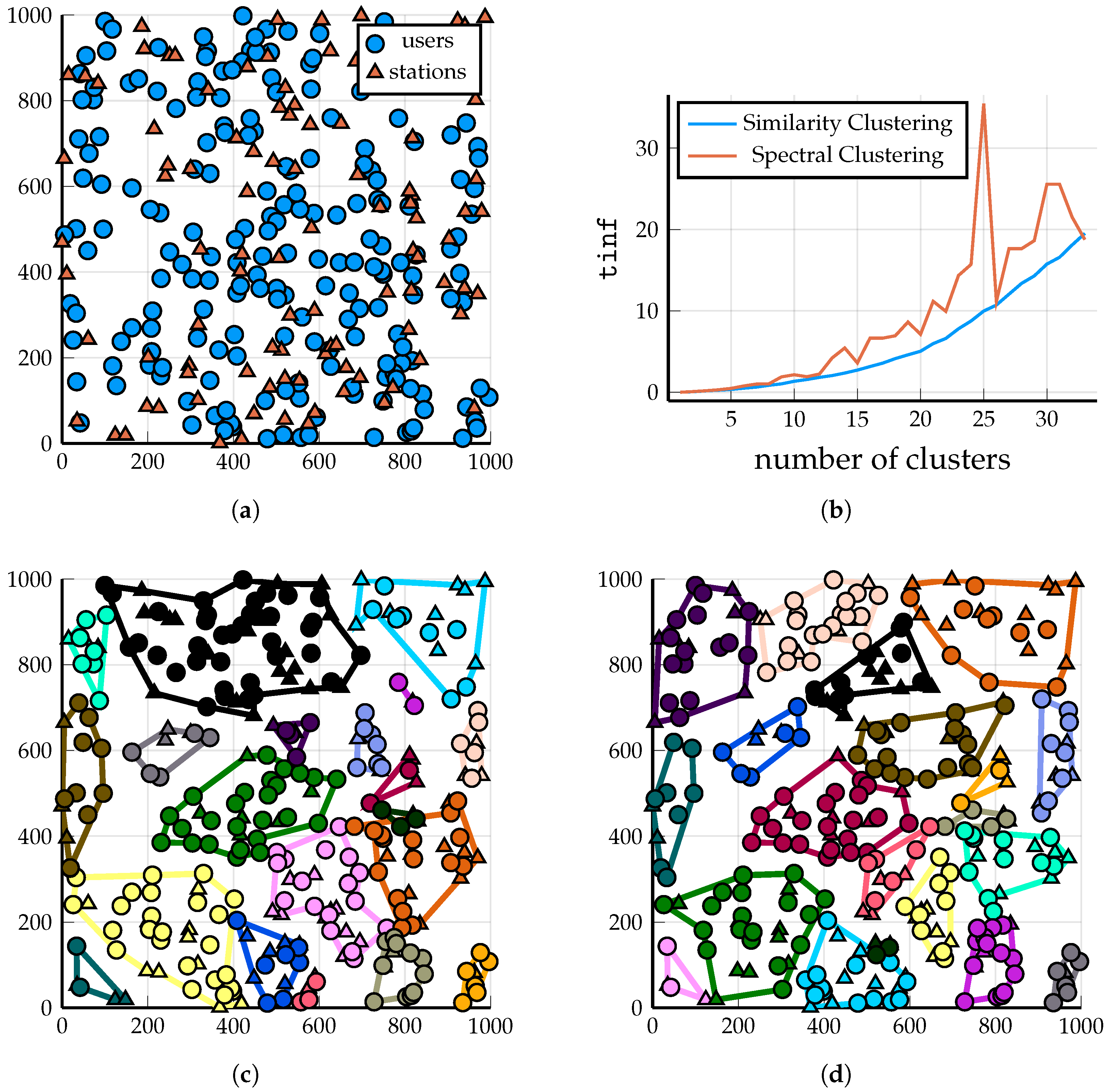
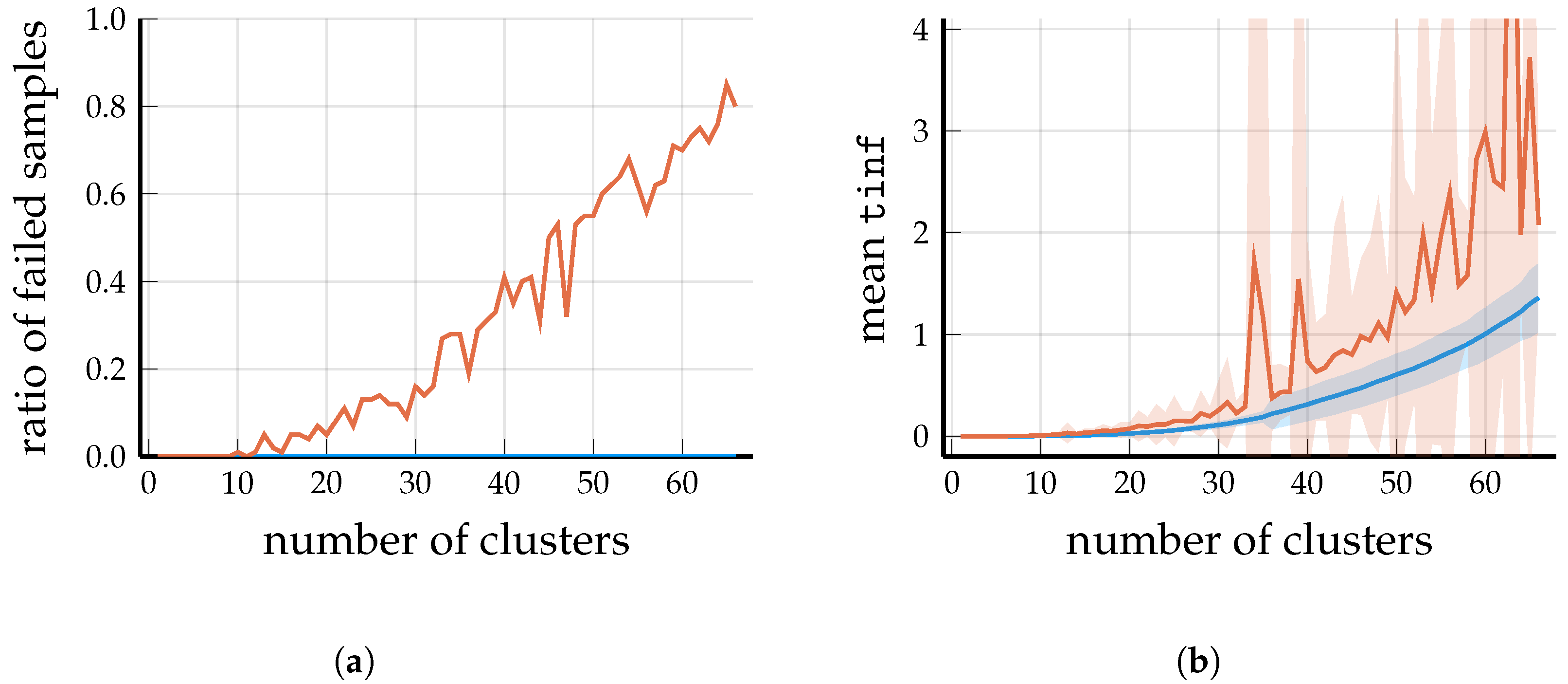
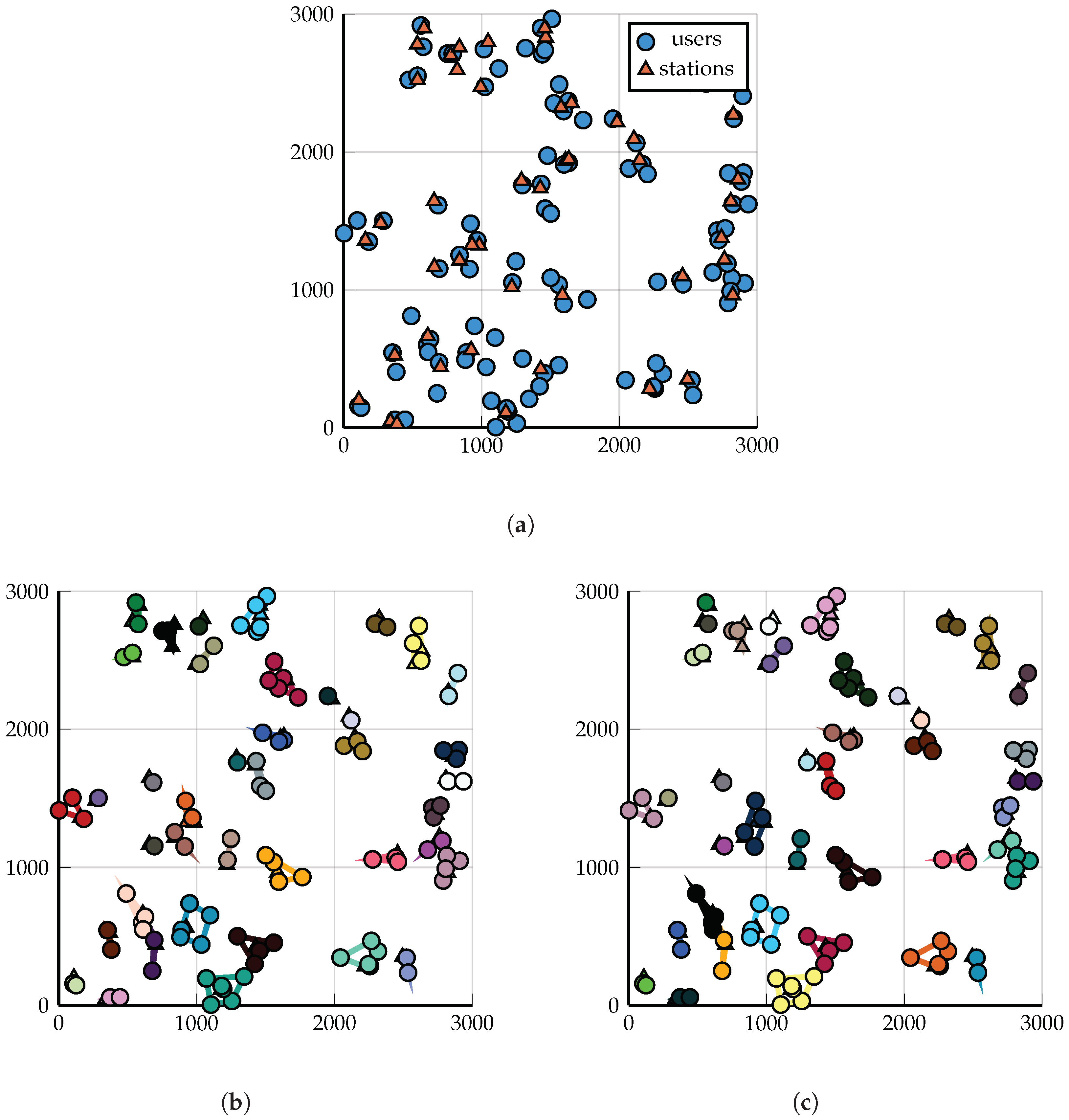
Figure 1.
Scenario 1: A demonstration of the output of the two clustering algorithms on 100 BSs and 200 users. Clustering solutions shown for
(so that the clusters are fairly large and visible). Triangles and circles represent BSs and users, respectively. (
a) A total of 100 BSs and 200 users, randomly and uniformly distributed. (
b) Comparison of the
values of the solution provided by the two algorithms as
M increases;
Spectral Clustering failed for
because it assigned a couple of users to a cluster without a base station. (
c) DP-Similarity Clustering into
clusters, Algorithm 2;
. (
d) Spectral Clustering into
clusters, see [
3];
.
DPH-clustering (Algorithm 1) is guaranteed to return an
M-part clustering of the base stations (if
). Consequently, the output of
DP-Similarity Clustering (Algorithm 2) is always an IF-cluster system (Definition 1) because it assigns each user to the cluster with the largest weight to the user; consequently, every user is served by at least one base station. However, this is not the case for
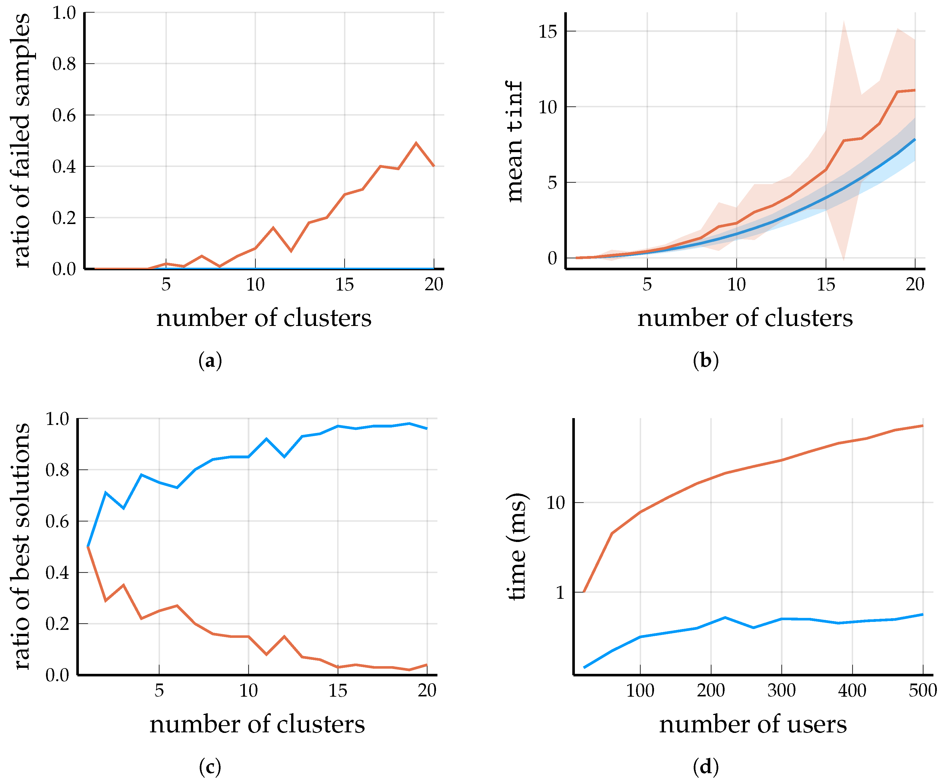
Spectral Clustering, which, in certain scenarios, is very likely to create a cluster with some users but zero base stations; see
Figure 2a and
Figure 3a.
4.1. Analysis of the Running Times
If the order of magnitude of
M is reasonable, i.e.,
, then the running times of neither
DP-Similarity Clustering nor
Spectral Clustering depend too much on the exact value of
M; in fact, the difference in running time between
clusters and
clusters with
BSs and
users is about
. Thus, the running times on
Figure 2d and
Figure 3d are measured for reasonable values of
M.
Recall Lemma 2. Theoretically, the running time of DP-Similarity Clustering is dominated by the matrix multiplication (computing the similarity measure), but this operation takes less than even for a matrix (thanks to the accelerated vector operations in the x86-64 instruction set). In this regime of , most of the running time of DPH-clustering (Algorithm 1) is spent after the matrix multiplication, which is log-quadratic in the number of base stations, but the constant factor of the main term is probably quite large. Thus, to improve the efficiency of the DP-Similarity Clustering algorithm, further development should be focused on DPH-clustering.
The running time of Spectral Clustering is a combination of computing the eigenvectors of a matrix of order and subsequently clustering the normalized eigenvectors via the k-means algorithm. Considering the large base matrix and the complex operations performed on it, it is not surprising that Spectral Clustering is an order of magnitude slower than DP-Similarity Clustering.
Let us refer back to our considerations after Problem 1. In real-world applications, users are constantly entering and leaving the network, and some of them may move out of the range of their cells. For this reason, the clustering needs to be frequently updated, but the time complexity may be prohibitive if the number of BSs is very large. However, if the overall changes to W are not large, it is possible to reuse , and thus DPH-clustering need not be called upon every time G or W is updated. Practically, DPH-clustering is called upon only if the value of the solution increases beyond a preset threshold. Since users are joined to the respective best cluster by Algorithm 2, if the users know the current , they can decide for themselves individually (locally) when to leave and join another cell.
4.2. Observations (Scenario 1)
Let us start with comparing the two algorithms (
DP-Similarity Clustering and
Spectral Clustering) on an arbitrarily chosen clustering problem in the setting of Scenario 1; after that, we turn to a quantitative comparison.
Figure 1a shows a randomly and uniformly generated placement of 100 BSs and 200 users. The scaling of the
(see Equation (
2)) of the solutions provided by
Spectral Clustering and
Spectral Clustering algorithm as a function of the number of clusters
M is shown in
Figure 1b.
Figure 2 and
Figure 3 compare the performance of the algorithms for
and 200 BSs. The plots correspond to the mean
values of the solutions provided by the algorithms over 100 random samples of BSs–user placements.
4.3. Observations (Scenario 2)
To cover a wider spectrum of parameters, for Scenario 2, we chose a non-uniform distribution for the base stations and set
to model a rural environment (see ([
1], Section 2)). The measured running times were not plotted because they mostly depend on the size of the matrix
W (and very weakly on
M). In fact, it turns out that the overall picture in Scenario 2 is very similar to Scenario 1.
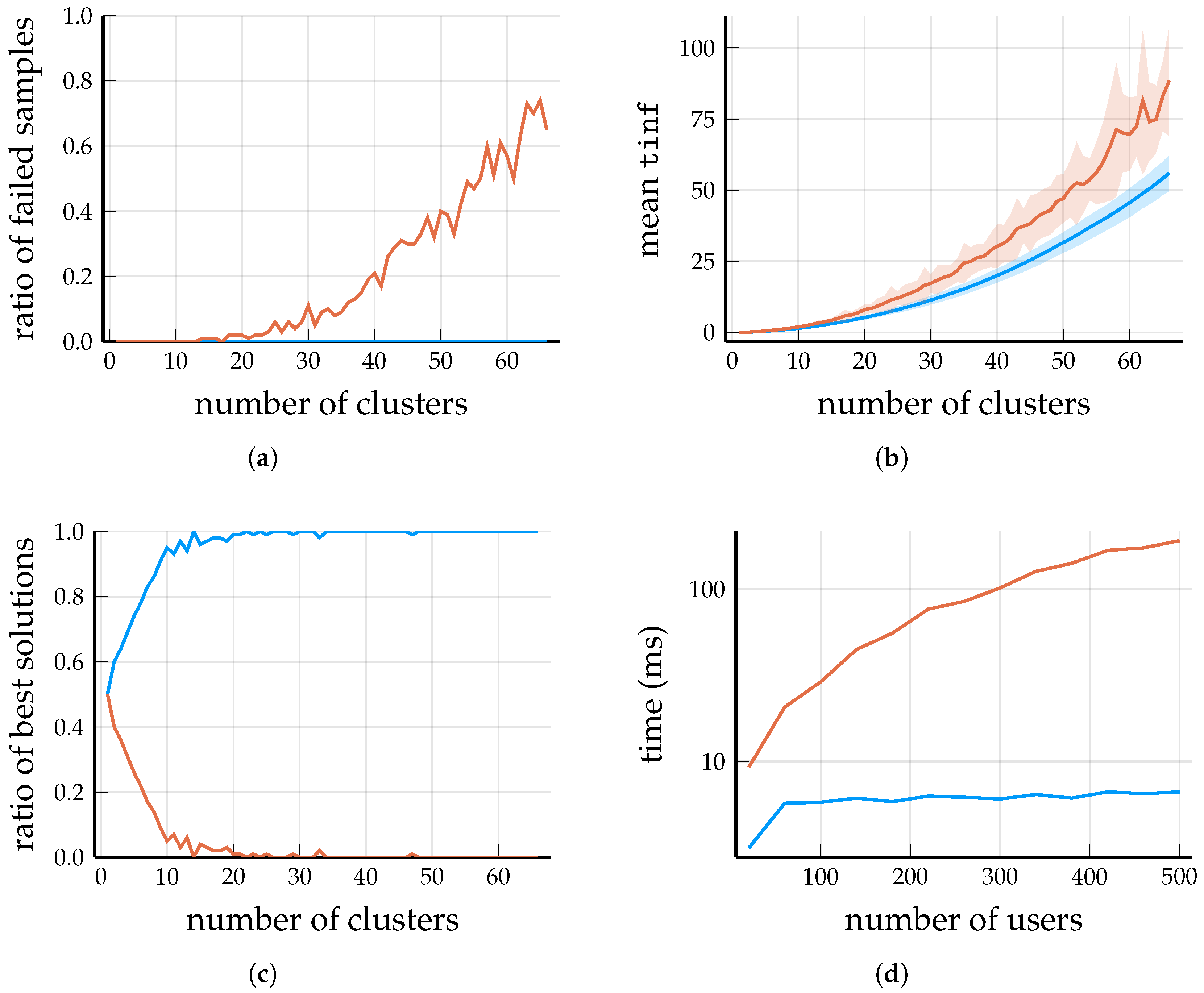
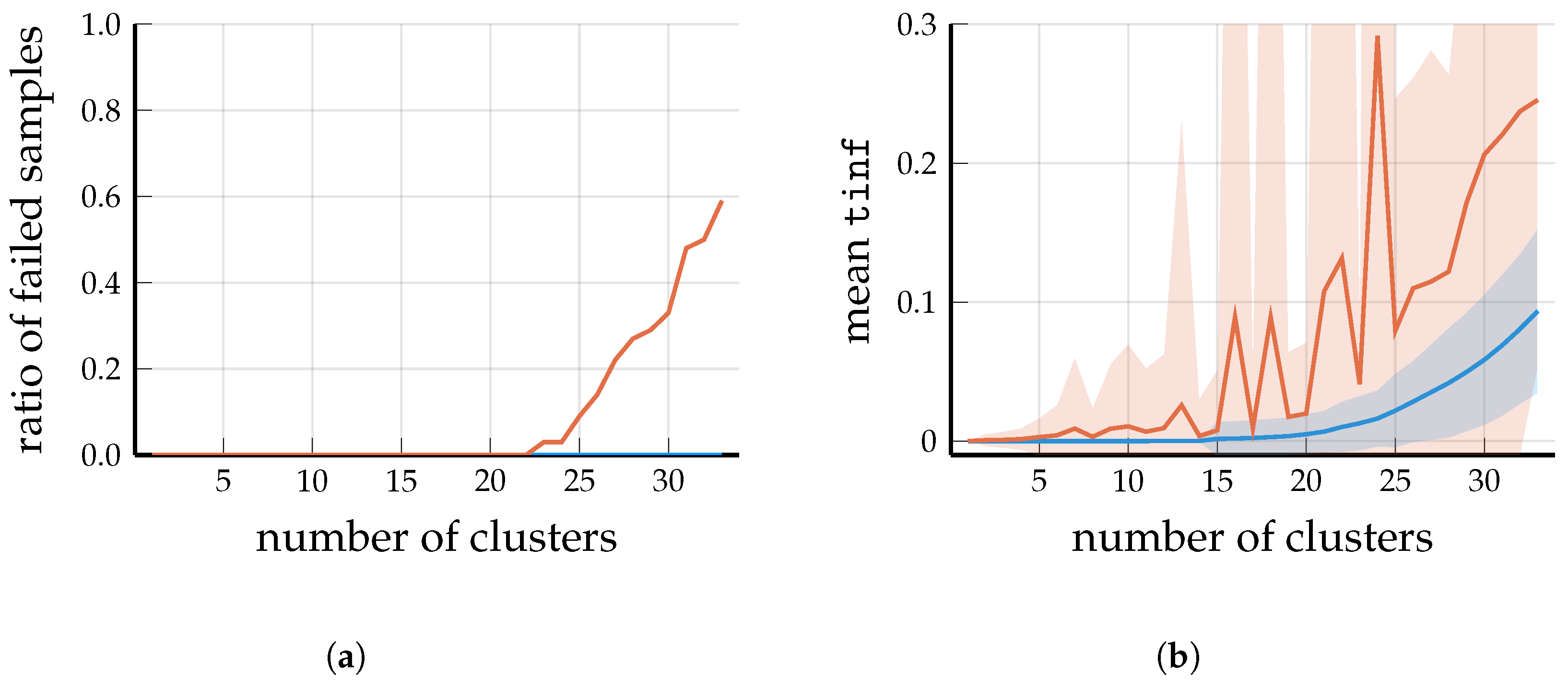
Figure 4a and
Figure 5a show that as the number of clusters grow, the higher the probability that spectral clustering generates an infeasible solution (containing a cluster without a base station). Even when a feasible solution is found by spectral clustering, most of them have a higher
value than the solution produced by Algorithm 2; see
Figure 4b and
Figure 5b. An example problem generated in the setting of Scenario 2 is visualized in
Figure 6, along with the solutions provided by similarity clustering and spectral clustering.
5. Conclusions
We proposed a robust and deterministic algorithm to solve the total interference minimization problem. We demonstrated through analysis and simulation that it provides higher quality solutions than the popular Spectral Clustering method (quality as measured by the value of the solution). The algorithm runs quickly enough to be considered in real-world applications.
The results of the different simulations plotted on the figures in the previous section demonstrate that our heuristic DP-Similarity Clustering algorithm provides high-quality solutions with low time complexity for the total interference minimization problem in bipartite graphs. Applying it for typical wireless networks, it nicely optimizes the total interference in the overall communication network. Compared with the state-of-the-art spectral clustering method, it is clear that the proposed algorithm achieves better performance with much less (computational) complexity.
Next, we list two suggestions for future research problems, whose solutions can considerably increase the usefulness of our algorithm in the wireless network domain.
The first problem is this: suppose that the clustering problem is restricted so that any cluster may contain at most T BSs; assume also that we want to have (at most) M clusters in the solution. However, prescribing both the upper bounds M and T may prevent the existence of feasible solutions, for example, if the number of base stations is more than . It is easy to construct examples where the greedy DPH-clustering algorithm (Algorithm 2) is not able to satisfy the two conditions simultaneously, even though many feasible solutions exist. It is very probable that some form of backtracking capability could help tremendously, but we have not tried to address this problem yet.
A more particular problem can be described as follows: our proposed algorithm assigns every BS to some cluster in the total interference minimization problem. However, it is possible that using a certain BS in any cluster causes more interference than not using it at all. This problem can be dealt with a trivial post-processing procedure: after the clustering is determined, delete base station i from if the removal decreases , since removing a BS from a cluster cannot increase the interference fractions of other clusters.


