Article

Three Metaheuristic Approaches for Tumor Phylogeny Inference: An Experimental Comparison

by
Simone Ciccolella
1,
Gianluca Della Vedova
1,*,
Vladimir Filipović
2 and
Mauricio Soto Gomez
3
1
Department of Computer Science, University of Milan-Bicocca, 20126 Milan, Italy
2
Faculty of Mathematics, University of Belgrade, 11000 Belgrade, Serbia
3
Department of Computer Science, Università degli Studi di Milano, 20133 Milan, Italy
*
Author to whom correspondence should be addressed.
Algorithms 2023, 16(7), 333; https://doi.org/10.3390/a16070333
Submission received: 3 June 2023 / Revised: 29 June 2023 / Accepted: 4 July 2023 / Published: 12 July 2023
(This article belongs to the Special Issue Algorithms for Natural Computing Models)

Abstract

:
Being able to infer the clonal evolution and progression of cancer makes it possible to devise targeted therapies to treat the disease. As discussed in several studies, understanding the history of accumulation and the evolution of mutations during cancer progression is of key importance when devising treatment strategies. Given the importance of the task, many methods for phylogeny reconstructions have been developed over the years, mostly employing probabilistic frameworks. Our goal was to explore different methods to take on this phylogeny inference problem; therefore, we devised and implemented three different metaheuristic approaches—Particle Swarm Optimization (PSO), Genetic Programming (GP) and Variable Neighbourhood Search (VNS)—under the Perfect Phylogeny and the Dollo-k evolutionary models. We adapted the algorithms to be applied to this specific context, specifically to a tree-based search space, and proposed six different experimental settings, in increasing order of difficulty, to test the novel methods amongst themselves and against a state-of-the-art method. Of the three, the PSO shows particularly promising results and is comparable to published tools, even at this exploratory stage. Thus, we foresee great improvements if alternative definitions of distance and velocity in a tree space, capable of better handling such non-Euclidean search spaces, are devised in future works.

1. Introduction

Inferring phylogenies is one of the key problems in bioinformatics, and its importance has increased more and more in recent years, as the availability of genetic data extracted from cancer samples has allowed researchers to examine how somatic mutations occur and, most importantly, accumulate during the progression of cancer. Furthermore, recent improvements in targeted therapies for cancer treatment require an accurate inference of the clonal evolution and progression of the disease to provide effective therapy [1,2].
Given the importance of the problem [3], several methods [4,5,6,7,8,9,10,11,12,13,14,15,16,17,18,19,20] designed to infer cancer progression from next-generation sequencing data have been published. The field has also recently witnessed the development of pipelines [21] and preprocessing steps.
Cancer cells proliferate in a highly constrained environment under very strong evolutionary pressure—for example, due to low levels of oxygen and the reaction of the immune system. This leads to frequently observed mutations that are very unusual in healthy cells [22], such as copy number aberrations, gene duplications, and ploidy changes. Some tools try to incorporate these mutational events when inferring tumoral evolutions (see, for example, [8,23]). While the predictions should become more accurate with such events included, the models become more complicated. Because the focus of this paper is a computational comparison, we do not consider these events, only the acquisition and loss of mutations.
On the other hand, single-cell sequencing data have provided clear evidence that mutation losses and (less frequently) mutation recurrences are common [24,25]. In fact, allowing only mutation accumulation corresponds to the directed perfect phylogeny problem on binary characters, which has a linear-time algorithm [26], while more general models (where mutation losses or recurrences are also allowed) result in NP-complete problems, with a much larger solution space. The perfect phylogeny model has found several applications in bioinformatics, most notably in haplotyping [27,28,29,30], and has been deeply investigated. For example, the combinatorial properties of perfect phylogenies are instrumental in the development of efficient algorithms, including the graph-theoretical characterization of genotype matrices that admit a tree representation [27,28,30,31].
In this paper, we focus on the Dollo-k model [5,32,33,34], which is a generalization of the perfect phylogeny model that incorporates the potential loss of characters. Under the Dollo-k model, each mutation can only be acquired once and lost at most k times in the entire evolutionary process. The restriction on the number of losses is motivated by the fact that even if character losses are possible, they are not frequent [24,35]. Variants of the Dollo-k model are considered in some recent tools, such as TRaIT [36], SiFit [37] and SPhyR [15], SASC [6], and ScisTree [38].
Notice that we are considering the binary case, where each mutation is either present or missing. The phylogeny inference problem under the Dollo-k model is NP complete [39], motivating the use of specialized metaheuristic strategies [6,15] which work well in practice even with fairly large instances. The fact that practical cases have incomplete or noisy information makes the use of heuristics more relevant [40,41]. Nonetheless, at least an exact solution for the problem, based on ILP, has been proposed [4], but it is too slow to be used in practice. To mitigate this problem, that tool has a hill climbing final step to guarantee that a local optimum is returned.
Given the success of nature-inspired metaheuristics in attacking various combinatorial problems and of a Simulated Annealing approach [6,42,43] to attacking the tumor phylogeny inference problem, we further investigate some additional approaches for inferring tumor phylogenies under the Dollo-k model, with the main goal of understanding which metaheuristics might be amenable to being the basis of future tools. More precisely, we investigate Particle Swarm Optimization [44], Genetic Programming [45], and Variable Neighbourhood Programming [
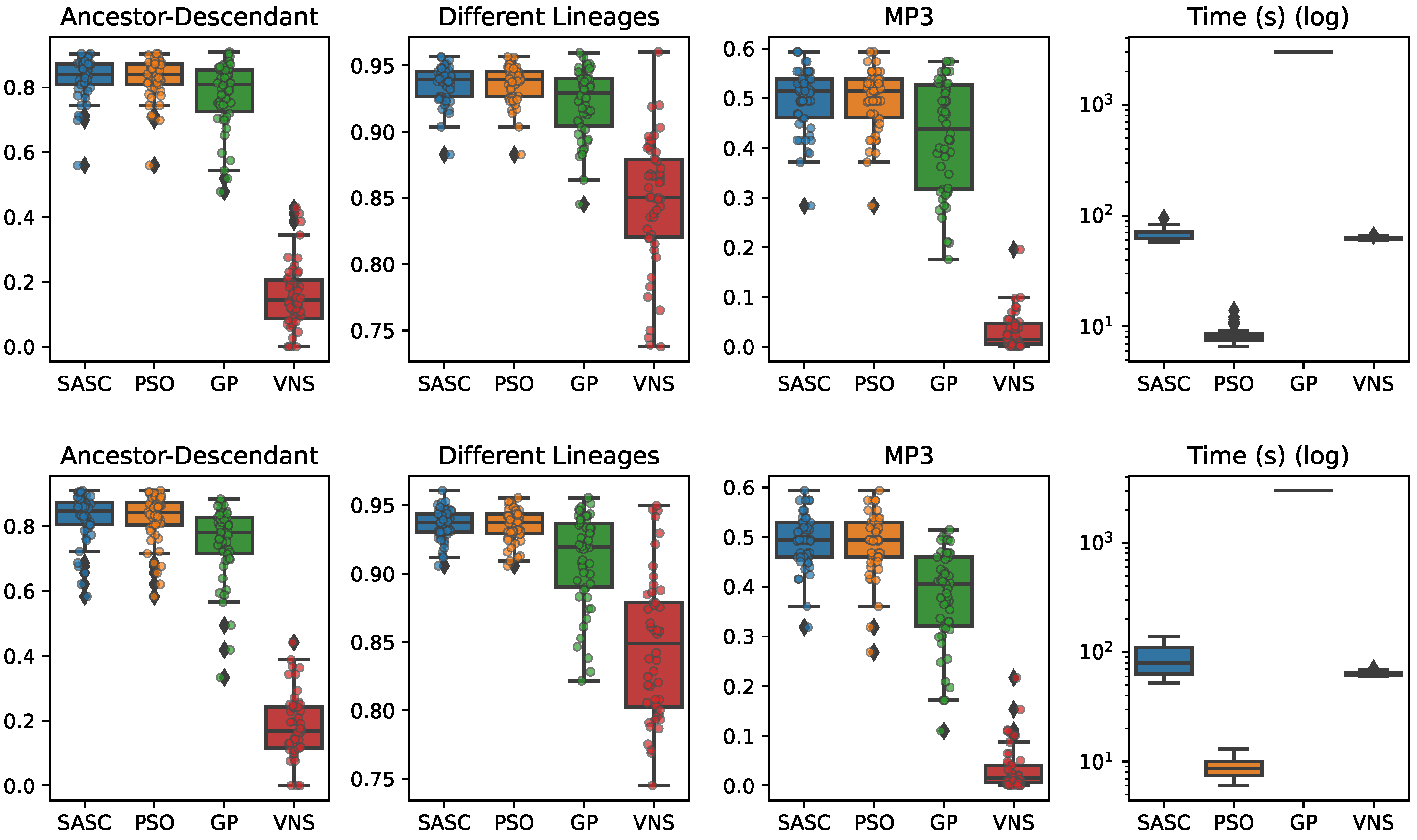
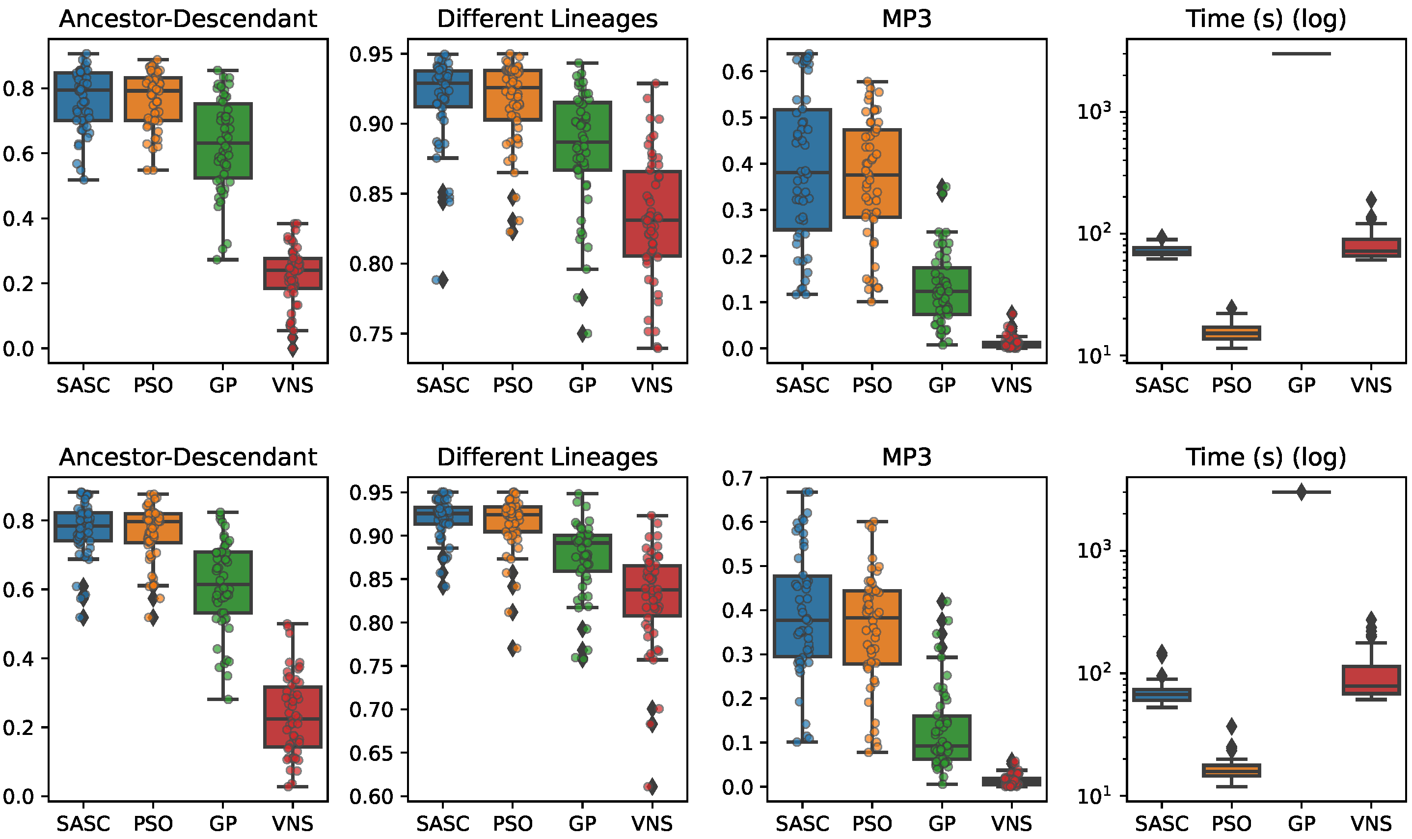
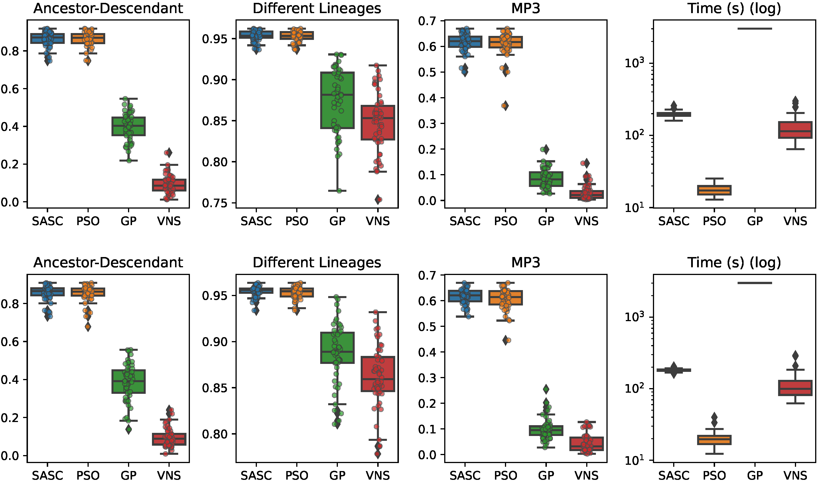
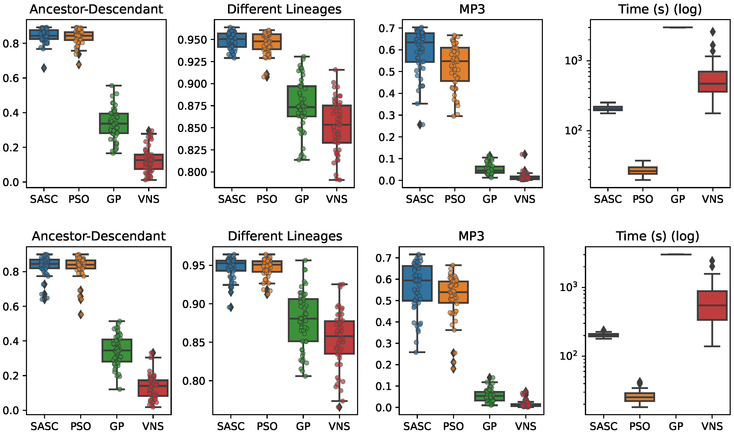
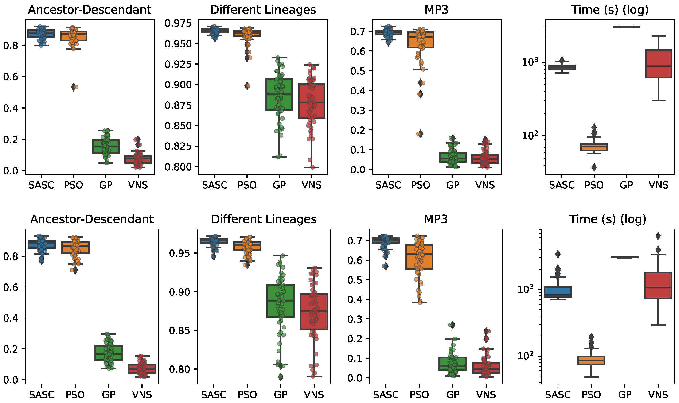
46]: the first two are population-based, while the third is trajectory-based. We test the proposed methods on six different synthetic datasets with different levels of complexity and evaluate their performance according to three different quality metrics, including one specifically designed for the evaluation of cancer progression [47]. The results show that Particle Swarm Optimization is roughly comparable with Simulated Annealing, while the results obtained via the other methods do not achieve the same level of accuracy.

2. Preliminaries

In this paper, we consider the computational problem of inferring a tumor phylogeny from single cell data in the presence of partial information. The input of the problem is an n × m ternary matrix I i j that represents the presence/absence of m mutations in n cells. The entries of I can assume three potential values: an entry I i j = 0 indicates that cell i does not have mutation j, I i j = 1 indicates the presence of mutation j in cell i, and a ? indicates uncertainty about the presence/absence of mutation j in cell i. The uncertainty in mutation presence within a cell is typically caused by insufficient coverage during sequencing.
Moreover, our models account for potential false positive and false negative entries in the input matrix, which are parameterized with a false positive/negative rate value. Specifically, let E denote the final n × m output matrix, which is the binary matrix without errors and noise estimated by the algorithm. We denote α j as the false negative rate of mutation j, and β as the false positive rate, similarly to [11,15,37,48]. Hence, for each entry E i j , the following holds:
P ( I i j = 0 | E i j = 0 ) = 1 β P ( I i j = 0 | E i j = 1 ) = α j
P ( I i j = 1 | E i j = 0 ) = β P ( I i j = 1 | E i j = 1 ) = 1 α j .
Notice that, due to the nature of the experimental measure, the false positive rate is usually low (around 10 6 ), while the false negative rate can be considerably higher (even 40 % ) [11,37,48]. Furthermore, each mutation can have a different false negative rate; for instance, a highly expressed gene will have significantly higher coverage than an under-expressed gene.
Similar to previous reconstruction methods ([6]), the objective of the reconstruction problem is to compute a matrix that maximizes the likelihood of the observed matrix I [48], assuming we know the probability rates of false positives, false negatives, and missing entries. This is conducted under the hypothesis that mutations in samples are acquired and lost following a specific evolutionary model.
A tumor phylogeny T on a set C of m mutations and n cells is defined as a rooted tree whose internal nodes are labeled by the acquisitions or losses of mutations from C, while the leaves are labeled by the cells.
The state of a node x is defined as the set of mutations c such that: (1) there is an ancestor of x where c is acquired, and (2) for each ancestor y of x where c is lost, there is a node of the path from y to x where c is acquired. Therefore, the state of each node x in the tree T can be represented as a binary vector of length m, called genotype profile and denoted by D ( T , x ) , where D ( T , x ) c = 1 if and only if the node x has the mutation j and 0 otherwise.
Given a binary matrix E, we say that a tree T encodes E if there exists a mapping σ of the rows (cells) of E to the leaves of T such that E i = D ( T , σ i ) for each row i of E, where σ i denotes the image of row i through the mapping σ . Informally, σ i is the node in the phylogenetic tree corresponding to the node where the cell i is attached. It is important to note that, given an input matrix I, the pair ( T , σ ) fully characterizes the output matrix E. Consequently, the reconstruction problem can be formulated as finding a tree T that maximizes the following objective function:
max j m i n log ( P ( I i j | D ( T , σ i ) j ) )
To simplify the computation of the likelihood, we make a slight abuse of notation by assuming that P ( I i j = ? | E i j = 1 ) = P ( I i j = ? | E i j = 0 ) = 1 . Furthermore, given a tumor phylogeny T, we can define the mapping σ as the one that maximizes the objective function. This means that σ can be computed directly from T, with T being the only variable in the optimization problem [6].

The Dollo-k Model

In this paper, we employ the Dollo-k evolutionary model, where each mutation can be acquired exactly once and lost at most k times throughout the entire tumor phylogeny tree [4]. The Dollo-0 and Dollo-1 models correspond to the perfect [26] and persistent [34] phylogeny models, respectively. The phylogeny reconstruction problem under a Dollo-k model is NP-hard [39] for any k > 1 .
Experimental evidence suggests that only a small number of mutation losses occur during the evolutionary process of each tumor [24]. To account for this observation, we introduce an additional constraint to our models, limiting the total number of mutation losses throughout the progression to a maximum of d occurrences. Alongside k, d is a parameter provided by the user.
In most of the cases studied, we set k 2 and d 5 . Furthermore, in our experiments, when the number of mutations is not too small, setting d 5 effectively implies that k 1 , making the parameter k redundant. However, we choose to retain it as it ensures that certain degenerate trees will never be computed.

3. Methods

3.1. Particle Swarm Optimization

The main idea of Particle Swarm Optimization [49] (PSO) revolves around maintaining a population of n feasible solutions (called particles). These particles move within the search space under the influence of the best overall solutions encountered by the entire population and the individuals themselves. Each particle is characterized by its position and its velocity. The population moves synchronously, with all individuals updating their positions and velocities simultaneously, until either convergence is achieved or a specified timeout is reached. The general outline of PSO is provided by Algorithm 1.
Algorithm 1: Particle Swarm Optimization
Algorithms 16 00333 i001
In our approach, each phylogeny is represented as a particle, with its topology serving as its position. Initially, positions are generated as random binary trees representing Perfect Phylogeny. At each iteration, particles can move using some of the following operations on a tree T and a node i, where ρ ( i ) denotes the parent of i in T:
  • Subtree Prune and Reattach: Given two internal nodes, u , v T , that are not ancestors of each other, we prune the subtree of T rooted in u by removing the edge ( u , ρ ( u ) ) . We then reattach this pruned subtree as a new child of v by adding the edge ( u , v ) ;
  • Add a deletion: Given two nodes u , v T such that v is an ancestor of u, we insert a node v in T to represent the loss of mutation v. The new node becomes the parent of u. Note that this operation is only performed if the resulting tree satisfies the desired phylogeny model. For the Dollo-k model, we must check that the mutation v has been lost in the tree at most k 1 times.
  • Remove a deletion: Given a node u T labeled as a loss, we simply remove it from the tree. All children of u are added as children of ρ ( u ) , then the node u is deleted.
  • Swap node labels: Given two internal nodes u , v T , the labels of u and v are swapped. If this operation renders a previously added loss invalid—because a mutation c is lost in a node c , but the node where the mutation c is acquired is no longer an ancestor of c —we remove the deletion c .
  • Subtree transplant: This operation requires an additional tree Q which does not necessarily contain the acquisition of all characters of T. The transplant involves: (1) deleting the subtree of T rooted at i (i.e., removing i and all its descendants), (2) making the root of Q a new child of ρ ( i ) (i.e., attaching Q to T), and (3) adjusting the resulting tree to ensure it is a Dollo-k phylogeny for the input mutations. The adjustment consists of two parts: (a) contracting a node corresponding to the loss of mutation c for each mutation c that has been lost more than k times, until c is lost k times in the tree, and (b) randomly adding a node for each input mutation that is not acquired in the tree. The resulting tree is guaranteed to be a Dollo-k phylogeny and a feasible solution to our problem.
To guide the update of particle positions, we introduce a new notion of distance. This distance, represented by Equation (1), is experimentally assessed and must be computed very rapidly to avoid degrading the performance of the method. This distance is computed by constructing a graph G whose vertex set is the union of vertices of two trees, T 1 and T 2 . Each edge e = ( v , w ) of G connects a vertex v of T 1 with a vertex w of T 2 . The edge is weighted with the number of mutations that are shared by the subtree of T 1 rooted at v and the subtree of T 2 rooted at w. To determine the distance between two trees, we compute a maximum weight matching M of the graph G. This matching establishes a one-to-one correspondence between the vertices of the trees, maximizing the overall number of shared mutations. To transform a matching into a suitable distance measure, we subtract the weight of M from the maximum number of mutations in either input tree, resulting in the following distance formulation:
d i s t ( T 1 , T 2 ) = max x T 1 m ( x ) , x T 2 m ( x ) max _ weight _ matching ( T 1 , T 2 ) .
This notion of distance is utilized to compute the velocity of the particles. The idea is that particles that are far from the local or the global optimum should have higher speed to encourage exploration. This higher velocity is determined by swapping subtrees within the tree, where the size of the swapped subtree is equal to the velocity. In other words, the higher the velocity of a particle, the larger the portion of the tree that gets replaced or modified during the optimization process.

3.2. Genetic Programming

Genetic programming (GP), introduced by Koza in 1992 [50], is population-based metaheuristics that has been successfully applied in various problem domains, including bioinformatics [51,52]. It is inspired by Genetic Algorithm (GA) and mimics natural selection and reproduction processes [53]. Both GP and GA imitate some spontaneous optimization processes in natural selection and reproduction. At each iteration (generation), GP manipulates a set (population) of encoded solutions (individuals). These individuals are evaluated using a fitness function, which represents the objective function. Based on their fitness, good individuals are selected to produce new solutions (offspring) through operators such as crossover and mutation. The offspring then replace some individuals in the current population. Extensive computational experience on several optimization problems shows that GA often produces high-quality solutions in a reasonable time [54,55]. We refer the interested reader to [56].
In this section, we present a GP approach (Algorithm 2) where each individual represents a feasible solution—a Dollo-k phylogeny. The same approach can be viewed as a GA, where the main difference between the two approaches is the representation of a solution. An individual in GA can be a string, while for GP, each individual is Dollo-k phylogeny.
In our implementation, a population size of 20 is used for smaller instances and 200 for larger instances. The halting criterion is a timeout of 3000 s on all instances. To maintain population diversity and avoid premature convergence, all individuals in the population are unique, meaning any duplicates are discarded.
Algorithm 2: Genetic Programming
Algorithms 16 00333 i002

3.2.1. Representation and Initialization

The initialization process of the GP approach ensures that only feasible solutions (Dollo-k phylogenies) are generated, similar to the PSO approach. The initialization starts by generating a random tree with a specific number of nodes, equal to the number of mutations (m), where no character is lost. This guarantees a fast and correct initialization, because each mutation is assigned one-to-one to a node. It is important to note that the initialization process allows for the exploration of the entire search space of feasible solutions. Any initial feasible solution can reach any other feasible solution in the search space through crossover and mutation operations. This property ensures that the GP approach has the capability to explore and search the space of Dollo-k phylogenies effectively.

3.2.2. Fitness Calculation

The fitness of an individual in the GP approach is primarily determined by its log-likelihood value, as described in Section 2. However, to prioritize simpler and smaller phylogenies over larger and more complicated ones, we consider some additional factors, such as the number of nodes s i z e ( T ) and the depth of the tree T d e p t h ( T ) in the definition of fitness. The fitness equation for an individual is as follows:
fitness ( T ) = L o g L i k e l i h o o d ( T ) + s i z e ( T ) 1000 + d e p t h ( T ) 100000 .
This definition of fitness helps prevent the occurrence of a phenomenon called bloat [57], which is the progressive growth of solutions, generation after generation, leading to larger and more complex individuals without a significant improvement in fitness.

3.2.3. Selection

The selection operator in GP determines which individuals will produce offspring in the next generation, based on their fitness. More precisely, individuals with higher fitness have a higher probability of being selected. Additionally, we employ an elitist strategy, where a few (in our case, one) highly fit individuals are directly passed to the new generation, while the selection process is applied to the remaining individuals to determine the rest of the population in the new generation. The individuals directly passed to the new generations are referred to as elite, while the others are classified as non-elite. The main effect of the elitist strategy is an emphasis on the exploitation phase. However, both elite and non-elite individuals play an equal role in the subsequent phases of the GP algorithm.
The selection procedure has a huge impact on the balance between the exploration phase, which focuses on finding new solutions, and the exploitation phase, which concentrates on the portion of the search space that has already been visited in the exploration phase. Finding an optimal balance between exploration and exploitation is crucial for the effectiveness of the GP algorithm.
The literature on selection operators [53] for GA and GP is rich and includes roulette wheel selection, ranking selection, and tournament selection. In this paper, we employ FGTS (fine-grained tournament selection [54]), which is an enhanced version of the standard tournament selection.
In the standard tournament selection, a tournament round is conducted for each non-elite individual that needs to be selected for the next generation. In each tournament round, a random subset of N t o u r non-elite individuals is chosen, and the fittest individual among them is selected as the winner. The winner is then passed on to the next generation, and a new tournament round begins. This process continues until the selection is complete. Notice that an individual can participate in multiple tournaments within a generation, which allows for fair competition among individuals and provides opportunities for selection based on their fitness in different contexts.
The tournament size N t o u r is typically an integer value that determines the balance between exploration and exploitation. Choosing an appropriate value for N t o u r can be challenging, as smaller sizes lead to slower convergence, while larger sizes result in faster convergence. To overcome this problem, FGTS introduces a rational (i.e., not necessarily integral) parameter F t o u r , which represents the desired average tournament size. In FGTS, tournaments can have different sizes, but the average size is maintained close to F t o u r . In our implementation, we have set F t o u r = 2.4 . The pseudocode for the selection operator is Algorithm 3.
Algorithm 3: Fine-grained tournament selection (FGTS)
Algorithms 16 00333 i003

3.2.4. Crossover

The crossover operator, also known as sexual recombination, introduces some variation in the population by combining genetic material from the parent individuals [56]. In the context of GP [50] for our problem, the crossover operator selects a random node—the crossover point—in each parent tree T 1 and T 2 . The crossover fragment for a parent T i is the subtree rooted at the crossover point. The offspring is created by replacing the crossover fragment of T 1 with the crossover fragment of T 2 —this operation can be seen as an extension to a pair of trees of the Subtree Prune and Regraft operation of the PSO. Additionally, a symmetric offspring is created by replacing the crossover fragment of T 2 with the crossover fragment of T 1 .
Designing a crossover operator for our problem is challenging because we need to guarantee that all offspring generated are feasible solutions. The crossover procedure involves the use of the function m a t e _ i n d i v i d u a l ( ) to create two offspring from the parents. The mating procedure must maintain the validity of the individuals in the population. The crossover procedure (Algorithm 4) starts by randomly selecting a mutation and checking if it can identify a valid crossover point in each tree. In other words, the crossover operation should result in two valid tumor phylogenies. If the check is successful, the offspring are created, and the procedure terminates. If the check fails, another mutation is selected, and the procedure is iterated.
It is important to note that the crossover operation is performed with a certain probability, known as the crossover probability, set to 0.9 in our approach.
Algorithm 4: Crossover
Algorithms 16 00333 i004

3.2.5. Mutation

Mutation is an asexual operator that operates on a single individual by modifying a specific mutation point. Many variants of the standard GP mutation have been presented in the literature.
In our approach, we have chosen one of the simplest mutation operations: the insertion of a new child of a given node and the deletion of a node—deleting a node x involves adding all its children as new children of the parent of the node x, then removing the node itself.
During the mutation process, each node of the individual is selected with a mutation probability that is smaller than the crossover probability. In our approach, the mutation probability is set to 0.1 . If a node is selected for mutation, there is an equal probability of either inserting a new child or deleting the node. This choice helps maintain the number of nodes in the individual and prevents excessive growth (bloat). If the resulting individual after a mutation is not a feasible solution, the mutation is discarded and the individual remains unchanged.

3.2.6. Additional Info about GP Algorithm and Implementation

We have implemented the GP algorithm in Python 3, using the DEAP library [58] for genetic programming, anytree for tree-like structures manipulation, and bitstring for the efficient manipulation of bit-arrays.

3.3. Variable Neighbourhood Programming

Genetic Programming and Particle Swarm Optimization are two population-based metaheuristics that explore the search space to find a near-optimal solution. However, they often converge slowly to a such a solution [59]. To address this issue, local search-based algorithms—where we apply a sequence of local changes to the current solution—have been developed. Variable Neighbourhood Programming (VNP) [60] is such a technique. VNP is inspired by automatic programming solution representation and Variable Neighbourhood Search (VNS) metaheuristics, combining the concept of neighborhood change with local search methods to ensure the discovery of local optima. Since VNP is based on non-binary representations, it should be more suited to problems on tree-like objects.
The main idea of VNS [46] and VNP is to change neighborhoods as the search progresses and incorporate local search methods to guarantee the identification of local optima. We refer the interested reader to [61]. The neighborhood structure plays a crucial role in defining the search space, both during the descent to local minima and in the escape from the valleys which contain them.
A fundamental ingredient of VNS and VNP is to define a suitable neighborhood structure for the solution space. In our case, we define four different neighborhoods for a given tumor phylogeny T. The first neighborhood, denoted by N 1 ( T ) , consists of all valid Dollo-k phylogenies that differ from T in a subtree whose root is a leaf, or a parent of a leaf, or a grandparent of a leaf. In other words, the root of such subtree has distance of at most 2 to a leaf. The second and third neighborhoods, N 2 ( T ) and N 3 ( T ) respectively, consist of all valid Dollo-k phylogenies that differ from T in a subtree whose root has a maximum distance of 5 (resp. 8) to a leaf. Finally, the last neighborhood, denoted as N 4 ( T ) , consists of all valid Dollo-k phylogenies. Notice that the cardinality of the neighborhoods decreases with increasing index (that is, | N s ( T ) | < | N s + 1 ( T ) | for each 1 s 3 ). To facilitate the presentation of the algorithm, we introduce the function z ( ) , where z ( 1 ) = 2 , z ( 2 ) = 5 z ( 3 ) = 8 , and z ( 4 ) = + . Each set N s ( T ) consists of all valid Dollo-k phylogenies that differ from T only in nodes with a distance at most z ( s ) to a leaf in T.
The main idea of VNP is alternating exploration of the current neighborhood through a local search, and the shaking, where we move to another neighborhood and different parts of the solution space can be explored. The pseudocode of VNP is given in Algorithm 5.
Algorithm 5: Variable Neighbourhood Programming
Algorithms 16 00333 i005
    The VNP follows a main loop that is iterated until a halting condition is met. Usually, this condition includes a limit on the number of iterations and a timeout for the overall execution time. In our case, the timeout is set to 3000 s for all instances. An important invariant of the algorithm is that T always is the best solution visited so far. The main loop consists of two phases: the shaking phase and the local search. In the shaking phase, a new solution T 1 is generated by exploring the current neighborhood, while the local search produces a solution T 2 . If T 2 is better than T, then T 2 becomes the new incumbent and the next search begins at the first neighborhood N 1 . However, if T 2 does not improve upon T, the algorithm progresses to the next neighborhood in the sequence to attempt further improvement. If the last neighborhood N 4 is explored and a solution better than the incumbent is found, the search restarts from the first neighborhood. Notice that the initial solution is a feasible solution computed as in Section 3.1 and that the fitness of a solution is computed as described in Section 3.2.2.

3.3.1. Shaking

The shaking phase in the VNP serves to introduce diversity and explore the current neighborhood N s ( T ) in search of a feasible solution T 1 . The shaking procedure typically involves the random extraction of a feasible solution. In our case, the definition of neighborhood classes, as described earlier, is tailored for the phylogeny sizes we expect to manage. Larger datasets would require a different definition of neighborhoods; for example, changing the subtree depth or introducing new classes.
Algorithm 6: Shaking
Data: s: current neighbourhood class. T: current solution.
Result: T 1 : a feasible solution
1 
T 1 c o p y ( T ) ;
2 
r a random vertex of T 1 that has distance at most z ( s ) to a leaf
3 
T | r the subtree of T 1 rooted at r
4 
T is a random tree with the same edge labels as T | r
5 
T 2 is obtained from T 1 by replacing T | r with T
6 
Contract in T 2 all edges of T labeled by a mutation loss c such that none of its ancestors is labeled c +
7 
return  T 2
In Algorithm 6, the shaking procedure selects a subtree T | r from the current solution T and permutes its edges. The selected subtree is denoted as T , and its edges are randomly rearranged to generate a new solution T 2 . Since T is a permutation of the edges of T | r , the set of mutation acquisitions and losses is preserved. The only possible case when T 2 is not valid only can happen when some mutation loss precedes a mutation acquisition. Line 6 of the algorithm explicitly removes such losses. The resulting tree is, therefore, a valid Dollo-k phylogeny.
The shaking procedure is designed to guarantee that all solutions in the search space can be potentially reached. This means that there are no feasible solutions that cannot be reached through the shaking procedure.

3.3.2. Local Search

Local search is performed on a shaken solution T 1 to potentially find an improved solution T 2 . Local search strategies commonly used in VNS and VNP include best improvement (highest descent) and first improvement (first descent). In our implementation, we have chosen the first improvement strategy for the local search. This means that the local search terminates as soon as the first improvement is found. The pseudocode for the local search with the first improvement strategy is presented in Algorithm 7.
Algorithm 7: Local search, first improvement strategy
Algorithms 16 00333 i006

3.3.3. Additional Info about VNP Algorithm and Implementation

The VNP algorithm is implemented as a Python 3 program using the anytree library for tree-like structures manipulation and the bitstring library for efficient bit-array manipulation.

4. Experimental Comparison

We conducted a total of seven experiments on simulated data. Each experiment involved generating 50 random trees with varying numbers of clonal expansions. These trees represented tumoral sub-populations sharing the same set of mutations. We further explored the impact of varying the number of losses randomly applied to the simulated phylogenies. This allowed us to evaluate the performance of the three methods described earlier in comparison to the reference method, SASC [6]. We notice that SASC is a heuristic based on Simulated Annealing.

4.1. Generation of the Datasets

To conduct our experiments, we followed the same generation methodology used in [4,6,62]. We generated 50 random clonal trees for each experimental setting. The generation process involved creating a random tree topology of S nodes. We iteratively added a new vertex as a child of a randomly selected node already in the tree, chosen uniformly at random. Once the topology was constructed, we randomly assigned N mutations as labels to the nodes. Each node was assigned at least one mutation. To allow deletions, we added up to k new nodes to the phylogeny. These new nodes were labeled as the loss of a random mutation acquired along the path from the node to the root. Next, we placed M cells in the tree by randomly selecting nodes. We computed the genotype profiles of these cells, which allowed us to obtain the profiles for our input matrix. Finally, we introduced random false negatives and false positive values into the input matrix, based on the probabilities α and β , respectively.
Since our main focus was on evaluating the performance of different meta-heuristics methods and their scalability on the Dollo-k and the Perfect Phylogeny model, we fixed the number of β to 0.00001 and varied the other parameters as described in Table 1.

4.2. Evaluation of the Results

Following established methodology [4,5,6,62], we evaluated the quality of the tree reconstruction inferred with the three novel algorithms using the following accuracy measures: Ancestor–Descendant accuracy and Different Lineage accuracy. Furthermore, we used the MP3 tree similarity measure [47], which is one of several recent notions of tree distances specifically designed for cancer phylogeny comparison in the literature [63,64,65,66]. We have chosen MP3, since it has already been used to test the accuracy of novel cancer inference methods [67].

4.2.1. Ancestor-Descendant Accuracy

For each pair of mutations ( a , b ) that are in an ancestor-descendant relationship in the simulated ground truth tree, we check if the same relationship is conserved in the inferred solution. If a pair is maintained, we consider it as a true positive; otherwise, it is considered a false negative; symmetrically pairs of nodes that are not in an ancestor-descendant relationship in the simulated ground truth tree can be true negatives or false positives. The accuracy is then defined as the F 1 measure over all pairs.

4.2.2. Different-Lineage Accuracy

As in the previous measure, we consider all pairs of mutation that are not in an ancestor-descendant relationship, i.e., they are on different evolutionary branches. Similarly to the previous measure, the score is the resulting F 1 measure over all pairs.

4.2.3. MP3 Tree Similarity

We also utilize the MP3 [47] similarity measure that is specifically designed to compare cancer phylogenies, and it is computed using the number of conserved triplets of mutations between the ground and the inferred trees.

4.3. Results

The three heuristics are compared against themselves and against SASC [6], which is considered the base reference for accuracy. Some interesting patterns clearly emerge as the complexity of the experimental setting increases. In general, when considering smaller input sizes, GP and VNS showed lower accuracy in all measures compared to PSO and SASC (Figure 1 and Figure 2). This difficulty in effectively exploring the search space became even more pronounced as the input size increased.
On the other hand, in all experiments, PSO exhibited ancestor–descendant and different lineages accuracy scores that were very close to those obtained by SASC. However, when considering the MP3 similarity measure, which is specifically tailored to tumor phylogenies, we observe a clear drop in performance (Figure 1, Figure 2, Figure 3, Figure 4, Figure 5 and Figure 6). Furthermore, none of the three methods are as accurate as SASC when employing a Dollo-3 model instead of a Perfect Phylogeny, again highlighting the need for better handling of the increasingly large search space.
In terms of efficiency, PSO was significantly faster than the other approaches, being 1 2 orders of magnitude more efficient in all experimental settings, except Experiment 7 (Figure 7. Experiment 7 was used in larger instances with a number of mutations increasing to 100 and 200. In this case, the faster execution of PSO was penalized by lower accuracy, according to all measures. Since no time constraint has been imposed on the algorithm, we conjecture that this drop in accuracy is due to difficulty in the exploration of the search space. In this experiment, we excluded GP and VNS due to the lack of performance in the previous results.
These results suggest that PSO could be a viable alternative to the Simulated Annealing heuristic. However, it may require a different definition of tree distance and more refined tuning to effectively manage the exploration phase.

4.4. Real Data

While the goal of this manuscript is the empirical analysis of different meta-heuristic approaches on simulated data, we also tested the PSO on a real dataset to show the applicability of the model in a real case scenario. Based on the previous experiments, we excluded GP and VNS. We selected an oligodendroglioma tumor; in particular, on patient MGH36 from [68], consisting of 77 SNVs, distinguished from PCR false positives using matched WES, over 579 cells. This tumor was already examined in [6].
Using PSO, we generated a Dollo-3 phylogeny for the patient, producing the solution shown in Figure 8. As depicted, the method infers a solution containing one deletion of IDH1; while no curated tree is available to compare it against, this shows the potential applicability of the PSO heuristic to real datasets.

5. Discussion

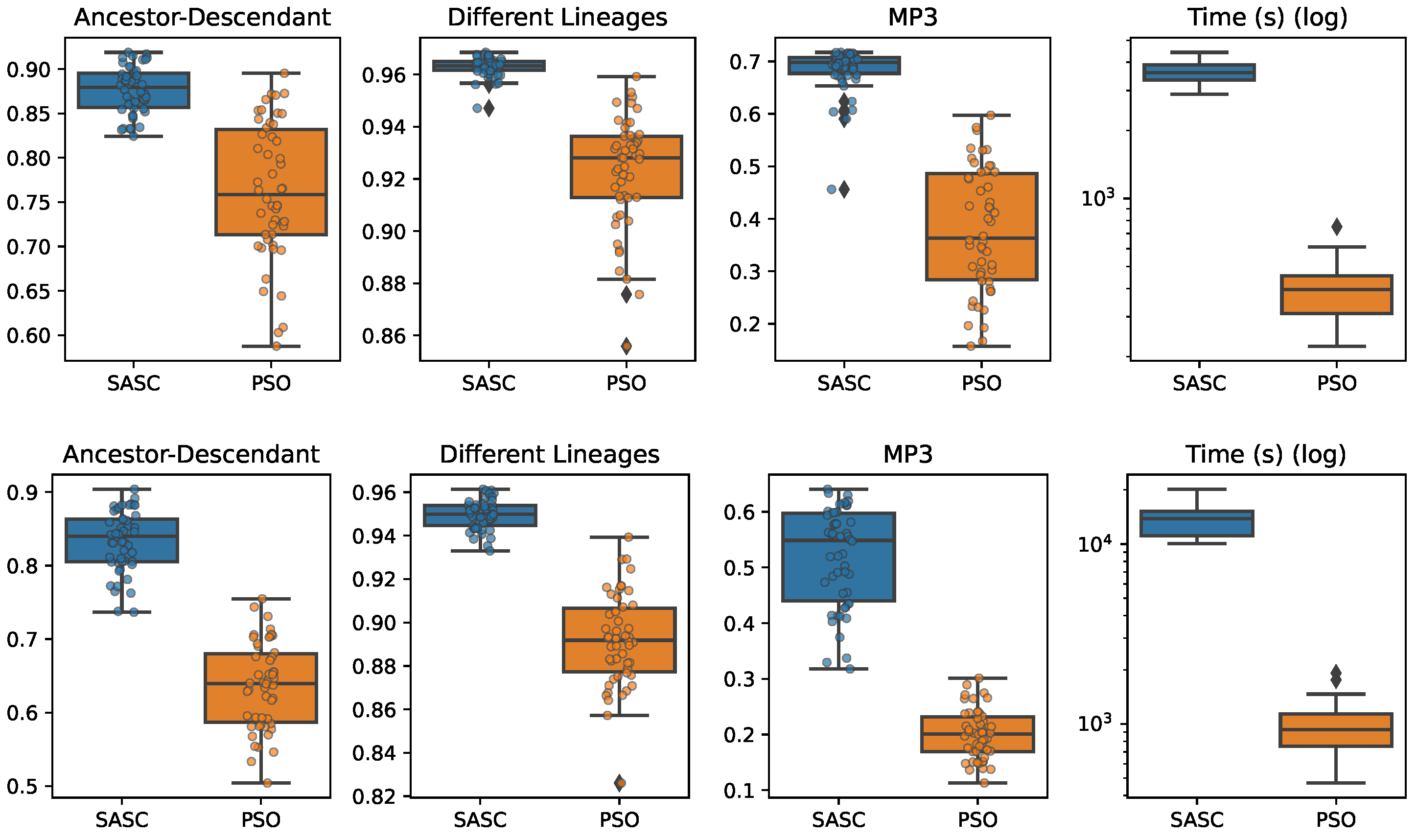
In this paper, we have presented and experimentally assessed three different metaheuristics (PSO, GP, and VNP) to infer tumor phylogenies under the Dollo model. We have compared these methods to the state-of-the-art Simulated Annealing approach (SASC).
Among the three metaheuristics, PSO showed the most promising results, although it was not able to outperform SASC. PSO demonstrated accuracy comparable to SASC in most experiments and measures, but its performance dropped as the complexity of the problem increased.
The main challenges faced by these methods stem from the fact that trees are not inherently a numeric space, which poses difficulties in defining distance, velocity, and direction on trees. Consequently, the design of appropriate definitions for these parameters is a crucial area for future research. These definitions should be computationally efficient and capable of capturing the properties that the PSO approach can exploit. Successful developments in this research direction have the potential to significantly enhance the accuracy of PSO. Moreover, we expect the parallelism capabilities of PSO to allow us to exploit many-cores infrastructures to allow an even larger exploration of the search space, leading to higher-accuracy tumor phylogenies.

Author Contributions

Conceptualization, S.C., G.D.V., V.F. and M.S.G.; methodology, S.C., G.D.V., V.F. and M.S.G.; software, V.F. and S.C.; validation, S.C.; formal analysis, S.C., G.D.V. and V.F.; investigation, S.C., G.D.V. and V.F.; resources, S.C. and G.D.V.; data curation, S.C. and G.D.V.; writing—original draft preparation, S.C., G.D.V. and V.F.; writing—review and editing, S.C., G.D.V., V.F. and M.S.G.; visualization, S.C.; supervision, G.D.V. and V.F.; project administration, G.D.V. and V.F.; funding acquisition, G.D.V. and V.F. All authors have read and agreed to the published version of the manuscript.

Funding

This project has received funding from the European Union’s Horizon 2020 research and innovation programme under the Marie Skłodowska-Curie grant agreement No 872539. Also, this research was partially supported by the Serbian Ministry of Education and Science under projects 174010.

Data Availability Statement

The implementation of the PSO is open source and available at https://github.com/IAL32/pso-cancer-evolution. The implementation of the GP and VNS is open source and available at https://github.com/vladofilipovic/documents-science-public within directory /journals/mdpi-algorithms-2023/prog. All the data used in the experimentation is available and reproducible at https://github.com/AlgoLab/meta_cancer, all accessed on 11 June 2023.

Acknowledgments

We thank Paola Bonizzoni, Aleksandar Kartelj and Murray Patterson for many enlightening discussions on this topic.

Conflicts of Interest

The authors declare no conflict of interest. The funders had no role in the design of the study; in the collection, analyses, or interpretation of data; in the writing of the manuscript; or in the decision to publish the results.

Abbreviations

The following abbreviations are used in this manuscript:
PSOParticle Swarm Optimization.
GPGenetic Programming.
GAGenetic Algorithms.
FGTSFine-Grained Tournament Selection.
SASimulating Annealing.
VNPVariable Neighbourhood Programming.
VNSVariable Neighbourhood Search.

References

  1. Morrissy, A.S.; Garzia, L.E.A. Divergent clonal selection dominates medulloblastoma at recurrence. Nature 2016, 529, 351–357. [Google Scholar] [CrossRef] [PubMed] [Green Version]
  2. Wang, J.; Cazzato, E.; Ladewig, E.; Frattini, V.; Rosenbloom, D.I.S.; Zairis, S.; Abate, F.; Liu, Z.; Elliott, O.; Shin, Y.J.; et al. Clonal evolution of glioblastoma under therapy. Nat. Genet. 2016, 48, 768–776. [Google Scholar] [CrossRef] [PubMed] [Green Version]
  3. Beerenwinkel, N.; Greenman, C.D.; Lagergren, J. Computational Cancer Biology: An Evolutionary Perspective. PLoS Comput. Biol. 2016, 12, e1004717. [Google Scholar] [CrossRef] [Green Version]
  4. Ciccolella, S.; Soto Gomez, M.; Patterson, M.D.; Della Vedova, G.; Hajirasouliha, I.; Bonizzoni, P. gpps: An ILP-based approach for inferring cancer progression with mutation losses from single cell data. BMC Bioinform. 2020, 21, 413. [Google Scholar] [CrossRef]
  5. Bonizzoni, P.; Ciccolella, S.; Della Vedova, G.; Soto Gomez, M. Does relaxing the infinite sites assumption give better tumor phylogenies? An ILP-based comparative approach. IEEE/ACM Trans. Comput. Biol. Bioinform. 2018, 16, 1410–1423. [Google Scholar] [CrossRef]
  6. Ciccolella, S.; Ricketts, C.; Soto Gomez, M.; Patterson, M.; Silverbush, D.; Bonizzoni, P.; Hajirasouliha, I.; Della Vedova, G. Inferring cancer progression from Single-Cell Sequencing while allowing mutation losses. Bioinformatics 2020, 37, 326–333. [Google Scholar] [CrossRef]
  7. Zaccaria, S.; Raphael, B.J. Accurate quantification of copy-number aberrations and whole-genome duplications in multi-sample tumor sequencing data. Nat. Commun. 2020, 11, 4301. [Google Scholar] [CrossRef]
  8. Satas, G.; Zaccaria, S.; Mon, G.; Raphael, B.J. SCARLET: Single-Cell Tumor Phylogeny Inference with Copy-Number Constrained Mutation Losses. Cell Syst. 2020, 10, 323–332.e8. [Google Scholar] [CrossRef]
  9. Malikic, S.; McPherson, A.W.; Donmez, N.; Sahinalp, C.S. Clonality inference in multiple tumor samples using phylogeny. Bioinformatics 2015, 31, 1349–1356. [Google Scholar] [CrossRef] [Green Version]
  10. Donmez, N.; Malikic, S.; Wyatt, A.W.; Gleave, M.E.; Collins, C.C.; Sahinalp, S.C. Clonality Inference from Single Tumor Samples Using Low Coverage Sequence Data. In Research in Computational Molecular Biology, Proceedings of the 20th Annual Conference, RECOMB 2016, Santa Monica, CA, USA, 17–21 April 2016; Singh, M., Ed.; Springer International Publishing: Cham, Switzerland, 2016; pp. 83–94. [Google Scholar]
  11. Ross, E.M.; Markowetz, F. OncoNEM: Inferring tumor evolution from single-cell sequencing data. Genome Biol. 2016, 17, 69. [Google Scholar] [CrossRef] [Green Version]
  12. Zafar, H.; Wang, Y.; Nakhleh, L.; Navin, N.; Chen, K. Monovar: Single-nucleotide variant detection in single cells. Nat. Methods 2016, 13, 505. [Google Scholar] [CrossRef] [Green Version]
  13. Zafar, H.; Navin, N.; Chen, K.; Nakhleh, L. SiCloneFit: Bayesian inference of population structure, genotype, and phylogeny of tumor clones from single-cell genome sequencing data. Genome Res. 2019, 29, 1847–1859. [Google Scholar] [CrossRef] [PubMed]
  14. El-Kebir, M.; Satas, G.; Oesper, L.; Raphael, B.J. Inferring the Mutational History of a Tumor Using Multi-state Perfect Phylogeny Mixtures. Cell Syst. 2016, 3, 43–53. [Google Scholar] [CrossRef] [Green Version]
  15. El-Kebir, M. SPhyR: Tumor phylogeny estimation from single-cell sequencing data under loss and error. Bioinformatics 2018, 34, i671–i679. [Google Scholar]
  16. Strino, F.; Parisi, F.; Micsinai, M.; Kluger, Y. TrAp: A tree approach for fingerprinting subclonal tumor composition. Nucleic Acids Res. 2013, 41, e165. [Google Scholar] [CrossRef] [PubMed] [Green Version]
  17. Sadeqi Azer, E.; Rashidi Mehrabadi, F.; Malikić, S.; Li, X.C.; Bartok, O.; Litchfield, K.; Levy, R.; Samuels, Y.; Schäffer, A.A.; Gertz, E.M.; et al. PhISCS-BnB: A fast branch and bound algorithm for the perfect tumor phylogeny reconstruction problem. Bioinformatics 2020, 36, i169–i176. [Google Scholar] [CrossRef]
  18. Satas, G.; Raphael, B.J. Tumor phylogeny inference using tree-constrained importance sampling. Bioinformatics 2017, 33, i152–i160. [Google Scholar] [CrossRef] [Green Version]
  19. Hajirasouliha, I.; Mahmoody, A.; Raphael, B. A combinatorial approach for analyzing intra-tumor heterogeneity from high-throughput sequencing data. Bioinformatics 2014, 30, i78–i86. [Google Scholar] [CrossRef] [Green Version]
  20. Popic, V.; Salari, R.; Hajirasouliha, I.; Kashef-Haghighi, D.; West, R.; Batzoglou, S. Fast and scalable inference of multi-sample cancer lineages. Genome Biol. 2015, 16, 91. [Google Scholar] [CrossRef] [Green Version]
  21. Ali, S.; Ciccolella, S.; Lucarella, L.; Della Vedova, G.; Patterson, M. Simpler and Faster Development of Tumor Phylogeny Pipelines. J. Comput. Biol. 2021, 28, 1142–1155. [Google Scholar] [CrossRef] [PubMed]
  22. Storchova, Z.; Pellman, D. From polyploidy to aneuploidy, genome instability and cancer. Nat. Rev. Mol. Cell Biol. 2004, 5, 45–54. [Google Scholar] [CrossRef] [PubMed]
  23. Zaccaria, S.; Raphael, B. Characterizing allele- and haplotype-specific copy numbers in single cells with CHISEL. Nat. Biotechnol. 2021, 39, 207–214. [Google Scholar] [CrossRef] [PubMed]
  24. Kuipers, J.; Jahn, K.; Raphael, B.J.; Beerenwinkel, N. Single-cell sequencing data reveal widespread recurrence and loss of mutational hits in the life histories of tumors. Genome Res. 2017, 27, 1885–1894. [Google Scholar] [CrossRef] [Green Version]
  25. Gawad, C.; Koh, W.; Quake, S. Dissecting the clonal origins of childhood acute lymphoblastic leukemia by single-cell genomics. Proc. Natl. Acad. Sci. USA 2014, 111, 17947–17952. [Google Scholar] [CrossRef] [PubMed]
  26. Gusfield, D. Efficient algorithms for inferring evolutionary trees. Networks 1991, 21, 19–28. [Google Scholar] [CrossRef]
  27. Gusfield, D. Haplotyping as perfect phylogeny: Conceptual framework and efficient solutions. In Proceedings of the 6th Annual Conference on Research in Computational Molecular Biology (RECOMB 2002), Washington, DC, USA, 18–21 April 2002; pp. 166–175. [Google Scholar]
  28. Bonizzoni, P. A Linear-Time Algorithm for the Perfect Phylogeny Haplotype Problem. Algorithmica 2007, 48, 267–285. [Google Scholar] [CrossRef]
  29. Satya, R.V.; Mukherjee, A. An Optimal Algorithm for Perfect Phylogeny Haplotyping. J. Comput. Biol. 2006, 13, 897–928. [Google Scholar]
  30. Ding, Z.; Filkov, V.; Gusfield, D. A Linear Time algorithm for Perfect Phylogeny Haplotyping (PPH) problem. J. Comput. Biol. 2006, 13, 522–553. [Google Scholar] [CrossRef] [Green Version]
  31. Gysel, R.; Gusfield, D. Extensions and Improvements to the Chordal Graph Approach to the Multistate Perfect Phylogeny Problem. IEEE/Acm Trans. Comput. Biol. Bioinform. 2011, 8, 912–917. [Google Scholar] [CrossRef] [PubMed]
  32. Farris, J.S. Phylogenetic Analysis Under Dollo’s Law. Syst. Biol. 1977, 26, 77–88. [Google Scholar] [CrossRef]
  33. Rogozin, I.; Wolf, Y.; Babenko, V.; Koonin, E. Dollo parsimony and the reconstruction of genome evolution. In Parsimony, Phylogeny, and Genomics; Oxford University Press: Oxford, UK, 2006. [Google Scholar]
  34. Bonizzoni, P.; Braghin, C.; Dondi, R.; Trucco, G. The binary perfect phylogeny with persistent characters. Theor. Comput. Sci. 2012, 454, 51–63. [Google Scholar] [CrossRef] [Green Version]
  35. Brown, D.; Smeets, D.; Székely, B.; Larsimont, D.; Szász, A.M.; Adnet, P.Y.; Rothé, F.; Rouas, G.; Nagy, Z.I.; Faragó, Z.; et al. Phylogenetic analysis of metastatic progression in breast cancer using somatic mutations and copy number aberrations. Nat. Commun. 2017, 8, 14944. [Google Scholar] [CrossRef] [PubMed] [Green Version]
  36. Ramazzotti, D.; Graudenzi, A.; De Sano, L.; Antoniotti, M.; Caravagna, G. Learning mutational graphs of individual tumor evolution from multi-sample sequencing data. BMC Bioinform. 2019, 20, 210. [Google Scholar] [CrossRef] [PubMed] [Green Version]
  37. Zafar, H.; Tzen, A.; Navin, N.; Chen, K.; Nakhleh, L. SiFit: Inferring tumor trees from single-cell sequencing data under finite-sites models. Genome Biol. 2017, 18, 178. [Google Scholar] [CrossRef] [Green Version]
  38. Wu, Y. Accurate and efficient cell lineage tree inference from noisy single cell data: The maximum likelihood perfect phylogeny approach. Bioinformatics 2019, 36, 742–750. [Google Scholar] [CrossRef]
  39. Goldberg, L.A.; Goldberg, P.W.; Phillips, C.A.; Sweedyk, E.; Warnow, T. Minimizing phylogenetic number to find good evolutionary trees. Discret. Appl. Math. 1996, 71, 111–136. [Google Scholar] [CrossRef] [Green Version]
  40. Benham, C.; Kannan, S.; Paterson, M.; Warnow, T. Hen’s teeth and whale’s feet: Generalized characters and their compatibility. J. Comput. Biol. 1995, 2, 515–525. [Google Scholar] [CrossRef]
  41. Steel, M. The complexity of reconstructing trees from qualitative characters and subtrees. J. Classif. 1992, 9, 91–116. [Google Scholar] [CrossRef]
  42. Černý, V. Thermodynamical approach to the traveling salesman problem: An efficient simulation algorithm. J. Optim. Theory Appl. 1985, 45, 41–51. [Google Scholar] [CrossRef]
  43. Kirkpatrick, S.; Gelatt, C.; Vecchi, M. Optimization by simulated annealing. Science 1983, 4598, 671–680. [Google Scholar] [CrossRef]
  44. Moscato, P. An introduction to population approaches for optimization and hierarchical objective functions: A discussion on the role of tabu search. Ann. Oper. Res. 1993, 41, 85–121. [Google Scholar] [CrossRef]
  45. Forsyth, R. BEAGLE A Darwinian Approach to Pattern Recognition. Kybernetes 1981, 10, 159–166. [Google Scholar] [CrossRef] [Green Version]
  46. Mladenović, N.; Hansen, P. Variable neighborhood search. Comput. Oper. Res. 1997, 24, 1097–1100. [Google Scholar] [CrossRef]
  47. Ciccolella, S.; Bernardini, G.; Denti, L.; Bonizzoni, P.; Previtali, M.; Della Vedova, G. Triplet-based similarity score for fully multilabeled trees with poly-occurring labels. Bioinformatics 2020, 37, 178–184. [Google Scholar] [CrossRef]
  48. Jahn, K.; Kuipers, J.; Beerenwinkel, N. Tree inference for single-cell data. Genome Biol. 2016, 17, 86. [Google Scholar] [CrossRef] [Green Version]
  49. Kennedy, J.; Eberhart, R. Particle swarm optimization. In Proceedings of the ICNN’95—International Conference on Neural Networks, Perth, Australia, 27 November–1 December 1995; Volume 4, pp. 1942–1948. [Google Scholar]
  50. Koza, J.R. Genetic programming as a means for programming computers by natural selection. Stat. Comput. 1994, 4, 87–112. [Google Scholar] [CrossRef]
  51. Taylor, J.; Rowland, J.J.; Gilbert, R.J.; Jones, A.; Winson, M.K.; Kell, D.B. Genetic Algorithm Decoding for the Interpretation of Infra-red Spectra in Analytical Biotechnology. In Proceedings of the Late Breaking Papers at EuroGP’98: The First European Workshop on Genetic Programming, Paris, France, 14–15 April 1998; Poli, R., Langdon, W.B., Schoenauer, M., Fogarty, T., Banzhaf, W., Eds.; CSRP-98-10. The University of Birmingham: Birmingham, UK, 1998; pp. 21–25. [Google Scholar]
  52. Langdon, W.B.; Buxton, B.F. Genetic Programming for Mining DNA Chip data from Cancer Patients. Genet. Program. Evolvable Mach. 2004, 5, 251–257. [Google Scholar] [CrossRef] [Green Version]
  53. Holland, J.H. Adaptation in Natural and Artificial Systems: An Introductory Analysis with Applications to Biology, Control, and Artificial Intelligence; MIT Press: Cambridge, MA, USA, 1992. [Google Scholar]
  54. Filipović, V. Fine-grained tournament selection operator in genetic algorithms. Comput. Inform. 2003, 22, 143–161. [Google Scholar]
  55. Kratica, J.; Kostić, T.; Tošić, D.; Dugošija, D.; Filipović, V. A genetic algorithm for the routing and carrier selection problem. Comput. Sci. Inf. Syst. 2012, 21, 49–62. [Google Scholar] [CrossRef]
  56. Rozenberg, G.; Bäck, T.; Kok, J.N. Handbook of Natural Computing; Springer: Berlin/Heidelberg, Germany, 2012. [Google Scholar]
  57. Langdon, W.B.; Soule, T.; Poli, R.; Foster, J.A. The evolution of size and shape. Adv. Genet. Program. 1999, 3, 163–190. [Google Scholar]
  58. Fortin, F.A.; De Rainville, F.M.; Gardner, M.A.; Parizeau, M.; Gagné, C. DEAP: Evolutionary Algorithms Made Easy. J. Mach. Learn. Res. 2012, 13, 2171–2175. [Google Scholar]
  59. Yao, X.; Liu, Y.; Lin, G. Evolutionary programming made faster. IEEE Trans. Evol. Comput. 1999, 3, 82–102. [Google Scholar]
  60. Elleuch, S.; Mladenovic, N.; Jarboui, B. Variable Neighborhood Programming: A New Automatic Programming Method in Artificial Intelligence; GERAD HEC Montréal: Montreal, QC, Canada, 2016. [Google Scholar]
  61. Hansen, P.; Mladenović, N. Variable neighborhood search: Principles and applications. Eur. J. Oper. Res. 2001, 130, 449–467. [Google Scholar] [CrossRef]
  62. Malikic, S.; Jahn, K.; Kuipers, J.; Sahinalp, S.C.; Beerenwinkel, N. Integrative inference of subclonal tumour evolution from single-cell and bulk sequencing data. Nat. Commun. 2019, 10, 2750. [Google Scholar] [CrossRef] [PubMed] [Green Version]
  63. Karpov, N.; Malikic, S.; Rahman, M.; Sahinalp, S.C. A Multi-labeled Tree Edit Distance for Comparing “Clonal Trees” of Tumor Progression. In Proceedings of the 18th International Workshop on Algorithms in Bioinformatics (WABI 2018). Schloss Dagstuhl-Leibniz-Zentrum fuer Informatik, Helsinki, Finland, 20–22 August 2018. [Google Scholar]
  64. Karpov, N.; Malikic, S.; Rahman, M.K.; Sahinalp, S.C. A multi-labeled tree dissimilarity measure for comparing “clonal trees” of tumor progression. Algorithms Mol. Biol. 2019, 14, 17. [Google Scholar] [CrossRef] [PubMed] [Green Version]
  65. DiNardo, Z.; Tomlinson, K.; Ritz, A.; Oesper, L. Distance measures for tumor evolutionary trees. Bioinformatics 2019, 36, 2090–2097. [Google Scholar] [CrossRef] [Green Version]
  66. Jahn, K.; Beerenwinkel, N.; Zhang, L. The Bourque distances for mutation trees of cancers. Algorithms Mol. Biol. 2021, 16, 9. [Google Scholar] [CrossRef]
  67. Sollier, E.; Kuipers, J.; Takahashi, K.; Beerenwinkel, N.; Jahn, K. Joint copy number and mutation phylogeny reconstruction from single-cell amplicon sequencing data. bioRxiv 2022. [Google Scholar] [CrossRef]
  68. Tirosh, I.; Venteicher, A.S.; Hebert, C.; Escalante, L.E.; Patel, A.P.; Yizhak, K.; Fisher, J.M.; Rodman, C.; Mount, C.; Filbin, M.G.; et al. Single-cell RNA-seq supports a developmental hierarchy in human oligodendroglioma. Nature 2016, 539, 309. [Google Scholar] [CrossRef] [Green Version]
Figure 1. Experiment 1: Perfect Phylogeny, Subclonal population size 5, Total number of mutations 15, Total number of cells 50, and (Top) α = 0.15 (Bottom) α = 0.20 . SASC and PSO score very similar in all measures. While there is a large gap between VNS and the other, GP is able to compare with the others. Running times vary between the methods, with PSO being at one to two orders of magnitude faster than the others.
Algorithms 16 00333 g001
Figure 2. Experiment 2: Dollo-3 Phylogeny, Subclonal population size 5, Total number of mutations 15, Total number of cells 50 and (Top) α = 0.15 (Bottom) α = 0.20 . SASC and PSO score very similar in all measures. While there is a large gap between VNS and the other, GP is able to compare with the others. Running times vary between the methods, with PSO being at one to two orders of magnitude faster than the others.
Algorithms 16 00333 g002
Figure 3. Experiment 3: Perfect Phylogeny, Subclonal population size 7, Total number of mutations 30, Total number of cells 100 and (Top) α = 0.15 (Bottom) α = 0.20 . SASC and PSO score very similar in all measures. On the other hand, GP and VNS start to show a clear drop in performance. Running times vary between the methods, with PSO being at one to two orders of magnitude faster than the others.
Algorithms 16 00333 g003
Figure 4. Experiment 4: Dollo-3 Phylogeny, Subclonal population size 7, Total number of mutations 30, Total number of cells 100 and (Top) α = 0.15 (Bottom) α = 0.20 . SASC and PSO score very similarly in all measures, except for MP3, in which we start to see a decrease in performance for the PSO. On the other hand, GP and VNS start to show a clear drop in performance. Running times vary between the methods, with PSO being at one to two orders of magnitude faster than the others.
Algorithms 16 00333 g004
Figure 5. Experiment 5: Perfect Phylogeny, Subclonal population size 9, Total number of mutations 50, Total number of cells 200 and (Top) α = 0.15 (Bottom) α = 0.20 . SASC and PSO score very similarly in all measures, except for MP3, in which we see a decrease in performance for the PSO. On the other hand, GP and VNS do not perform comparably to the other two algorithms. Running times vary between the methods, with PSO being at one to two orders of magnitude faster than the others.
Algorithms 16 00333 g005
Figure 6. Experiment 6: (Top) Dollo-3 Phylogeny, Subclonal population size 9, Total number of mutations 50, Total number of cells 200 and (Top) α = 0.15 (Bottom) α = 0.20 . SASC and PSO score very similarly in all measures, except for MP3, in which we see a decrease in performance for the PSO. On the other hand, GP and VNS do not perform comparably to the other two algorithms. Running times vary between the methods, with PSO being at one to two orders of magnitude faster than the others.
Algorithms 16 00333 g006
Figure 7. Experiment 7: (Top) Dollo-3 Phylogeny, Subclonal population size 9, Total number of mutations 100, Total number of cells 200 and α = 0.15 . (Bottom) Dollo-3 Phylogeny, Subclonal population size 9, Total number of mutations 200, Total number of cells 200 and α = 0.15 . While PSO is significantly faster than SASC (one order of magnitude) it lacks in performance according to all measures when compared to SASC. On the other hand, GP and VNS were excluded from the experiments due to low accuracy in previous experiments.
Algorithms 16 00333 g007
Figure 8. Tree inferred by PSO for the oligodendroglioma MGH36 from [68]. The tree was computed employing a Dollo-3 phylogeny model. In this picture, a red node indicates a loss of mutation.
Algorithms 16 00333 g008
Table 1. Parameters used for dataset generation. S is the size of the subclonal population, N is the total number of mutations generated, M is the total number of cells, and k is the value of the Dollo-k model, i.e., in our experiments we have considered either a Perfect Phylogeny or a Dollo-3 Phylogeny.
Experiment #SNMk α
15155000.15, 0.20
25155030.15, 0.20
373010000.15, 0.20
473010030.15, 0.20
595020000.15, 0.20
695020030.15, 0.20
79100, 20020030.15
Disclaimer/Publisher’s Note: The statements, opinions and data contained in all publications are solely those of the individual author(s) and contributor(s) and not of MDPI and/or the editor(s). MDPI and/or the editor(s) disclaim responsibility for any injury to people or property resulting from any ideas, methods, instructions or products referred to in the content.

