Developing Prediction Model of Travel Times of the Logistics Fleets of Large Convenience Store Chains Using Machine Learning

Abstract

Convenience store chains are many people’s top choice for dining and leisure and have logistics procedures that involve each store receiving multiple deliveries because of the varying delivery periods and suitable temperatures for different goods. The estimated arrival time for each delivery has a huge impact on the route arrangement and convenience store preparation for dispatchers to schedule future deliveries. This study collected global positioning system travel data from a fleet of one of the top convenience store chains in Taiwan between April 2021 and March 2022 and proposed machine learning to establish a model to predict travel times. For unavailable data, we proposed the nonlinear regression equation to fill in the missing GPS data. Moreover, the study used the data between April 2022 and September 2022 with mean absolute percentage error to validate the prediction effects exceeding 97%. Therefore, the proposed model based on historical data and the machine learning algorithm in this study can help logistics fleets estimate accurate travel times for their scheduling of future delivery tasks and arranging routes.

1. Background

Convenience stores have become an integral part of modern life because of changes in lifestyles and consumption habits. Convenience stores are mostly located near commercial areas or communities with convenient transportation. In addition to providing daily supplies, such stores offer other services, including fee collection and e-commerce product delivery, and are open 24 h daily. Since the coronavirus pandemic began in 2019, the importance of convenience stores has increased in Taiwan because they have facilitated the reservation and sale of medical masks through a name-based mask distribution system, the reservation of vaccines, and the reservation and distribution of stimulus vouchers. According to the open data platform of convenience stores in Taiwan [1], Taiwan has 13,173 convenience stores in service as of May 2023, with one store for every 1789 people on average.

A single convenience store that runs 24 h daily might receive up to eight deliveries of stocks in a day because of the varying delivery temperature requirements of different products and the need to provide the freshest foods and meals at the store. For example, room-temperature, frozen, refrigerated, fresh, and microwave foods are delivered in separate vehicles at their required storage temperatures.

The logistics of chain convenience stores follow a predetermined schedule. With the varying sales levels across convenience stores as well as the opening and closing of stores nearly every week, delivery dispatchers formulate a delivery plan for the following month according to each store’s average monthly order quantity and expected monthly delivery. The dispatch process involves three main operations:

(1)

Planning a delivery route that connects various stores to be served by a vehicle: The goal is to maximize vehicle capacity without exceeding the loading limit, to minimize the distance between stores along the route, and to arrive at each store at its expected delivery time. Convenience stores are typically located at crossroads or in densely populated areas, which makes deliveries by large vehicles difficult. Therefore, deliveries for these stores are usually completed using medium-sized vehicles that weigh 10 metric tons when loaded. Each delivery route contains approximately 10–20 stores, and the expected time to complete delivery on a route is approximately 3 h.

(2)

Sequencing the stops at convenience stores: This task involves a traveling salesman problem that requires the route to satisfy each store’s expected delivery time and minimize the travel distance by sequencing stops in an appropriate order.

(3)

Estimating the expected arrival time for each delivery and notifying the corresponding store in advance: This task is particularly helpful for convenience store logistics because convenience stores are typically located at crossroads or in densely populated areas and might have specific requests regarding delivery times because of the nature of deliveries, which makes it difficult for delivery vehicles to avoid traffic. In addition, the absence of storefront space for trucks to park and unload because of these stores’ proximity to large roads means that trucks can only park and unload at roadsides. Therefore, upfront notifications to the stores allow them to make space for delivery trucks to park, for delivery to be transported in stores, and for storing the delivery.

Operations (1) and (2), which concern the delivery vehicle’s route planning, are outside the scope of this study and are thus to be discussed in depth in a separate study. The current study focuses on constructing a model that estimates travel time for logistics vehicles.

The currently available online map resources that provide estimated arrival time based on users’ departure points and destinations include OpenStreetMap, Google Maps, and navigation applications. Google Maps’ estimated travel time is particularly accurate because it included real-time traffic. The convenience store chain investigated in this study until May 2023, which has seven warehouses and 3980 store locations, has 15,892,182 (3987 × 3986) possible combinations between any two points. 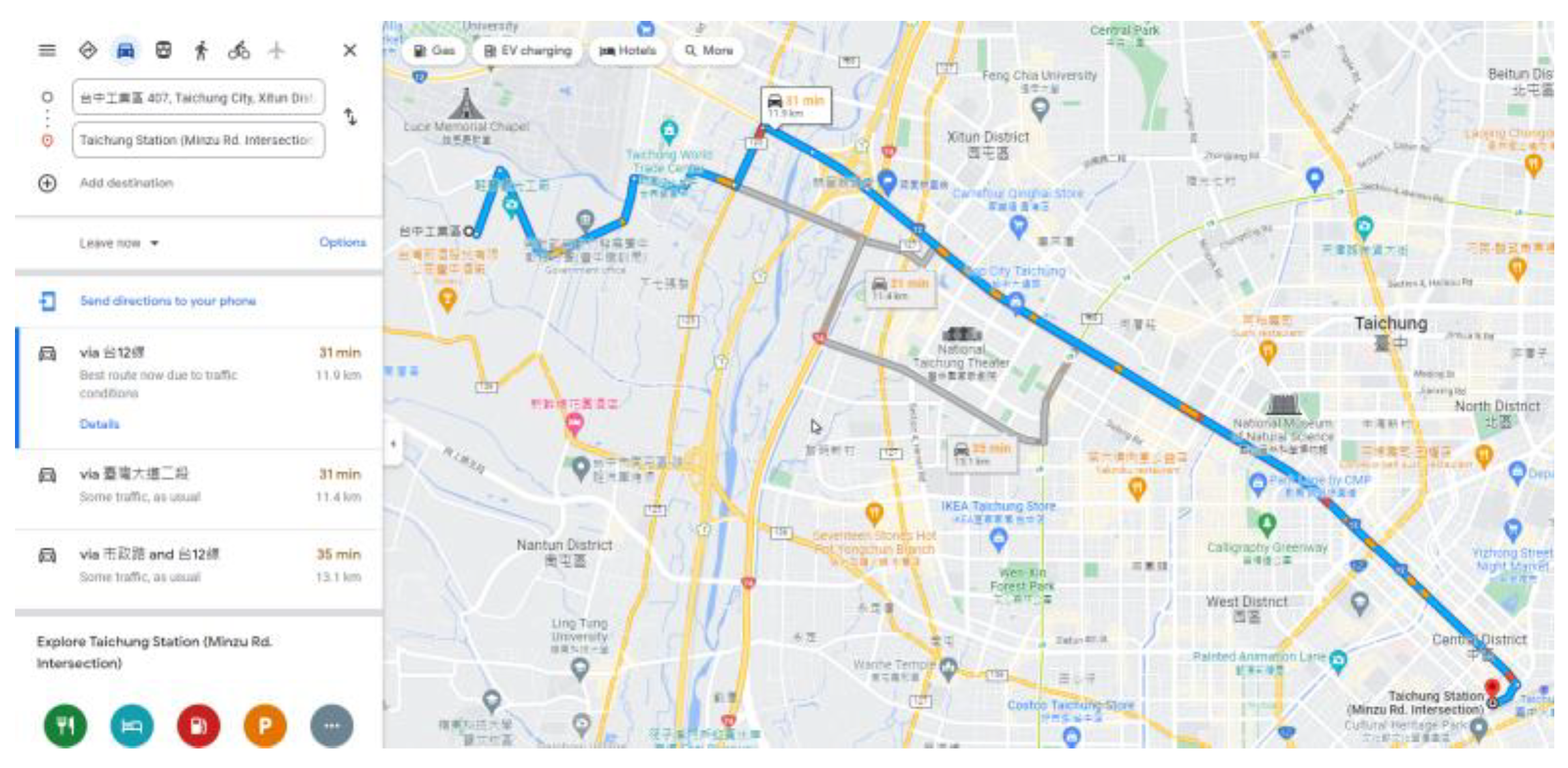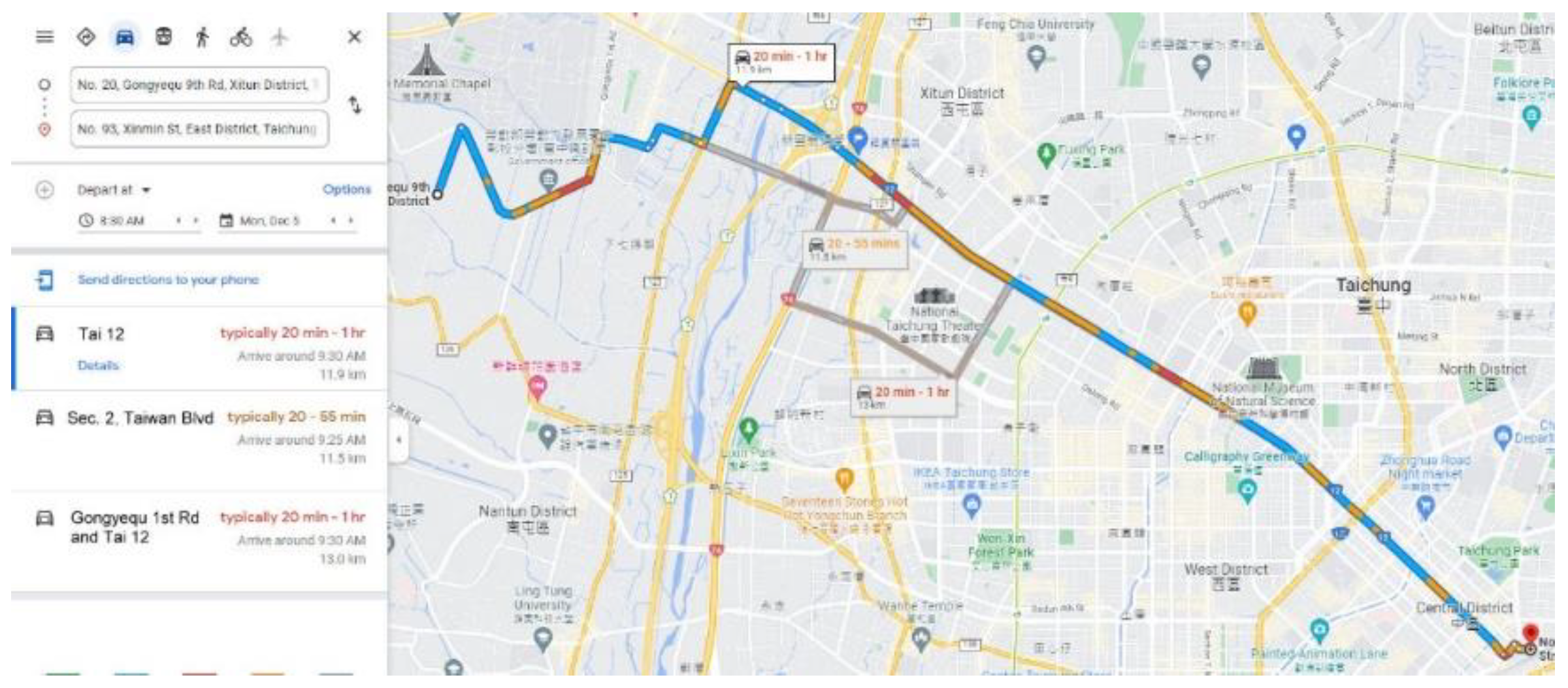Based on the Google Map API rate on 1 May 2023, it will cost US$158,921 (US$10 per 1000 elements) to build a two-dimensional road matrix. Moreover, Google Maps provides estimations for passenger cars but not for trucks, which are the target of this study and are slower than passenger cars. This study aimed to schedule future vehicle dispatches rather than plan routes for immediate departure. However, for a future departure, Google Maps provides a range of estimated travel times, with the shortest travel time being up to three times shorter than the longest travel time; thus, future dispatch scheduling based on Google Maps estimations is a difficult task. Consider the example of a journey from the Taichung Industrial Park to the Taichung Railway Station (Figure 1 and Figure 2). For immediate departure at 08:30, the estimated travel time is 31 min (1860 s); however, for departure at 08:30 on later dates, the estimated travel time is 20 min to 1 h (1200 to 3600 s).

Accordingly, we were not to discuss the accuracy of other map resources in predicting the future travel time in this study. The main purpose was to establish a prediction model that did not rely on other map resources, and this study used the global positioning system (GPS) travel history of the target logistics fleet as training data to build the model to proceed with future dispatch scheduling that can obtain a more accurate prediction. This study collected the actual driving speeds and coordinates being acquired for subsequent discussions. The travel time estimations were applicable to the target fleet.

The subsequent sections discuss the topics as follows. Section 2 provides a literature review of travel time estimation, travel records of logistics fleets, track logs, and machine learning. Murphy (2012) [2] explained that machine learning is to use approaches to automatically detect patterns in data and to use the uncovered patterns to predict data or other results. Thus, machine learning can be used in this study. In Section 3, this study mainly develops predictive analytics based on machine learning. The target logistic fleet serves one of the largest convenience store chains in Taiwan, and this study collected the target fleet’s GPS travel history for one year to conduct statistical analyses for estimating the travel time matrix between every two points at different times of the day for establishing an intervallic road network. To ensure the quality of matrix data, the standard deviation, sample, and reference ratio we designed are used to filter data with poor reliability. For some periods without data collected, the predicted travel time can be obtained by the nonlinear regression equation. Section 4 shows actual travel time records for six months between April 2022 and September 2022 using the mean absolute percentage error (MAPE) to validate the prediction effects of the model. Section 5 discusses the travel time of schedule of future deliveries and Section 6 gives the conclusion of the prediction model of travel times using machine learning.

2. Literature Review

Many studies have performed travel time estimation by using different methods, including spanning trees, regression analysis, neural networks, and machine learning methods. In these studies, usable data were collected in advance to construct a prediction model to estimate the travel time. Prediction models have been constructed using various methods and algorithms. For delivery tasks with different departure times, intervallic travel time estimation is particularly helpful for scheduling future delivery tasks and managing these tasks in real time.

According to relevant research, collecting data is an essential step when addressing the travel time problem. Suitable algorithms can be used with large quantities of data to construct models for travel time estimation. The essential data that must be collected include departure location, departure time, arrival location, arrival time, and route taken in historical travel. These data may be sourced from manual documentation at the times of delivering out and receiving deliveries, the times shown on the driver’s package-checking device, the coordinate data sent out from delivery vehicles’ GPS devices, or charge-coupled device camera data on vehicle entries and exits at the loading or unloading locations. In this study, travel history generated on the basis of coordinate data were collected from the GPS devices of delivery vehicles to estimate the travel times between two points at different hours.

Collecting the actual travel records of logistics fleets is difficult. Previous relevant studies have rarely used actual travel data for analysis, and most of them have adopted open data published by governmental institutions, such as the average travel speed and the speed limit of roads. The actual travel records of logistics fleets include records on delivered and received goods, which can include the names of the owners of the goods and information on the goods. Such information is unsuitable for open distribution and research. Therefore, this study used the coordinates recorded by the satellite positioning equipment on vehicles and eliminated vehicle identification data, such as vehicle plate numbers. Information on only the origin, departure time, destination, and arrival time was used in this study to obtain the travel times between two locations on a route during different periods. Numerous data samples were collected in this study, and unreasonable outliers were excluded to obtain the average travel time on a route during different periods. The average travel time can be used to estimate the travel time on a route during a specific period.

To estimate the arrival time of vehicles, geographic information technology must be used to convert coordinates into locations. Rapid advances have been achieved in geographic information systems (GISs), and these systems are currently applied in different domains, particularly transportation and traffic. The conversion of a set of coordinates (x, y) into a location by a GIS is known as geocoding or map matching. Common map matching methods based on vector data include the puncture method and scanning method, which involve calculations. Large numbers of coordinates are converted into locations in transportation problems of large logistics fleets, and these coordinates cause a high load on the system and server. In this study, the number of GPS tracks was more than 65 million. Therefore, an excellent calculation method was required to analyze a large quantity of data in a short time. Many studies have been conducted on map matching. Mu et al. [3] proposed the conversion of vector data into raster data and the use of a look-up table for rapidly finding the location corresponding to a set of destination coordinates from each pixel in the raster data. Their method was more efficient than the conventional puncture method. White et al. [4] proposed a map matching algorithm based on the coordination between user location and basic maps. Quddus et al. [5,6] integrated GPS data with dead reckoning data to develop a map matching algorithm with the extended Kalman filter and the spatial digital database of a road network. Kuijpers et al. [7] used a map matching algorithm with the space-time prism and k-shortest path algorithms. Zhang et al. [8] proposed a map matching system based on the evaluation of similar trajectories. Brakatsoulas et al. [9], Kong and Yang [10], Hashemi and Karimi [11], and Liu et al. [12] have proposed different improvements for map matching based on road filters and road trajectories. In this study, OpenStreetMap (OSM) was used as the reference for road data. Liu et al. [13] and Fan et al. [14] have performed comprehensive research on the usage of road data and geographic information in OSM. Increasing the data calculation and processing speed is crucial when performing statistical analysis on a large quantity of data. Yao and Li [15] proposed the use of big spatial vector data to improve the efficiency of data storage and organization, spatial index, data processing, and spatial analysis. Li et al. [16] proposed using massive floating car data for traffic surveillance to solve data-intensive geospatial problems for urban traffic systems. Zheng et al. [17] proposed using MapReduce to improve the computation performance of spatial data models. Lopes et al. [18], Loidl et al. [19], and Pfoser et al. [20] have proposed using spatial regression models, geo-visualization techniques, and vehicle position management to construct spatial and transportation models and improve the computation performance when using spatial data. Guan and Clarke [21] proposed using a parallel raster processing programming library to reduce the computation time when using spatial data. Sun et al. [22] used a spatial index based on raster data and extracted the geometric features of geographic objects corresponding to the raster to improve the positioning, searching, and querying performance.

Concerning studies related to travel time prediction, Wang et al. [23] proposed a wide deep recurrent learning model, which comprised train-wide models, deep neural networks, and recurrent neural networks, to estimate the travel time for a fixed route and departure time. Ahmed et al. [24] proposed an explainable artificial intelligence method to evaluate and compare different prediction models and to explain the effects of temporal and spatial characteristics on travel time. Servos et al. [25] used extremely randomized trees, adaptive boosting, and support vector regression (SVR) to solve problems with a small quantity of data in a short time. Qiu and Fan [26] conducted short-term travel time prediction and examined the prediction accuracies of the Regional Integrated Transportation Information System, decision trees, random forest, extreme gradient boosting, and a long short-term memory neural network for the spatial and temporal characteristics of travel time. Servos et al. [25] used machine learning, extremely randomized trees, adaptive boosting, and SVR to construct models for travel time prediction. They then evaluated a model established for predicting multimodal container transport between the United States and Germany. Building on their research, this study conducted a regression analysis to estimate the travel time matrix for periods in which travel history was unavailable. Luo and Spieksma [27] determined the minimum travel time and minimum total latency when serving multiple requests. They proposed the match-and-assign algorithm and compared its performance with that of other transportation algorithms. Xu et al. [28] used vehicle trajectory data on an expressway to analyze the effectiveness of time scales, tolerance, and series length for the estimation of travel time. They also compared the prediction results obtained using the autoregressive integrated moving average method and a backpropagation neural network. Tsai [29] used k-nearest neighbor method to investigate the travel time on highways. They analyzed and compared the traffic information collected by an electronic toll collection system and vehicle detectors. Tsai examined how the traffic data were affected by the time and vehicle detector. The aforementioned studies used different methods within a specific period to perform research, and few studies have estimated the travel time between the same origin and destination in different periods. Therefore, in the present study, the travel times at different periods were determined. Webb et al. [30] proposed that reliability be estimated according to the conception and estimation of reliability under the framework of classical test theory. On the basis of this suggestion, the present study determined a reference ratio for filtering data according to the data frequency and the difference between the data collected by this study and those obtained from the target fleet’s electronic map.

In this study, track logs, which included the coordinates recorded by the satellite positioning equipment on vehicles, were used. After spatial judgment, the track logs included information on the origin, departure time, destination, and arrival time. Filjar et al. [31] proposed an advanced calculation method for determining the accuracy and error of the coordinates determined through satellite positioning. This method reduces the ionospheric delay, tropospheric delay, and satellite clock error of the Global Navigation Satellite System (GNSS) at the cost of increasing the computational complexity. Iliev et al. [32] indicated that the radio signals of the GNSS have extended routes because they are reflected and refracted, Therefore, the measured distance changed, and multipath errors occurred. The aforementioned authors found that multipath errors and ionospheric delay have strong effects on the precision, and they proposed using choke ring antennas to reduce multipath errors. In this study, the travel time was investigated, and all the coordinates in the track logs were collected from the same satellite positioning equipment and expected to have the same errors. Therefore, the errors were expected to cancel each other out; thus, no corrections were made to any GNSS coordinate. Studies that require precise positioning may consider using correction mechanisms for the aforementioned errors.

Liu et al. [33] used the machine learning method to predict the online taxi-hailing demand, and use RMSE, MAPE, and R square to evaluate the performance. Almalki et al. [34] used machine learning technology for research on correlations between the COVID-19 pandemic with socioeconomic, food access, and health problem variables by applying linear and nonlinear regression models. The GIS analysis was also for comparison. The results of machine learning and GIS had the same directions and indicated the correlation between the dependent variables and independent variables. The source data of this study are GPS driving records, and the travel time records obtained from the analysis are from GIS data. Regarding [33,34], this study uses MAPE to verify the prediction effects based on the regression model. Nguyen and Seidu [35] used ten machine learning algorithms to plan the predictive maintenance strategy of the sewer network and used a ratio of 80/20 to split the data set, 80% for building the model, and 20% for validating and selecting the sewer condition assessment model. This study referred to the splitting concept from [35] and adopted the ratio of 12/6, i.e., 12 months for model building and 6 months for model validation. Kostrzewski (2020) [36] developed a simulation model from randomly generated orders and analyzed the sensitivity of parameters. The study [36] discussed the impact of different orders in the simulation model under different parameters and included methods for model construction, data collection and analysis, and conclusions for sensitivity analysis. Thus, this study referred to the above methods and proposed a reference rate method to handle filtering outliers. Thompson et al. (2023) [37] discussed the simulation model measurement of the complexity and used different indicators or combinations to measure the model structure, number of variables, model parameters, the logical process which were integrated into Kolmogorov complexity (KC) and normalized compression distance (NCD) values to quantify the complexity of the model.

The above literature discussed that GPS driving records were transferred into travel time between two locations, the outliers of travel time were filtering, and the predictions using machine learning and historical travel time records to verify the model accuracy.

3. Research Method

This study developed a distance matrix that encompasses the warehouses from which delivery vehicles depart and all the stores served. Moreover, it determined the distances and travel times between each two points in the matrix. If N is the total number of stores, then the total number of points in a road network is N + 1 (including the warehouse). The number of combinations of data on travel distances and times is (N + 1) × N (the travel distance and travel time between a point and itself are 0). For delivery task scheduling, the developed two-dimensional matrix allowed for quick checks on the travel time and distance between any two points within them, according to which the route and sequence of deliveries can be determined to minimize the total travel time of the fleet and to ensure that deliveries arrive at each store by the expected delivery time. Assume that unloading time is proportional to the number of goods to be unloaded at each store. In this case, the time of a vehicle’s arrival at a store should be accurately estimated by summing the vehicle’s unloading time at the preceding store and the time required to travel to the particular store.

All the vehicles in the target fleet have a GPS device on board that sends the vehicle’s GPS information, including GPS time, speed, latitude and longitude, and azimuth, to the management system every 30 s. According to this information, the management system detects abnormal vehicle activities, such as speeding, prolonged stop at a location, or deviation from the scheduled route. The information relevant to this study is the times a vehicle enters and exits a location, including the warehouse and stores. The management system delineates the areas of the warehouse and stores to establish geofences for them. A vehicle is considered to have arrived at and departed from a location at the moment it drives into and outside the geofence, respectively. Given that many convenience stores are located near a crossroad, the management system might incorrectly detect a vehicle’s arrival at a store if it enters the store’s geofence as it drives past the store. To address this problem, this study included two additional factors—pulling the parking brake and stopping for 3 min or longer—for determining a vehicle’s arrival. Specifically, a vehicle was determined to have arrived at a store for unloading the delivery if it entered the store’s geofence if the parking brake was pulled, and if it had stopped at the spot for 3 min or longer, with the arrival time being recorded as the time the vehicle first entered the geofence. The vehicle was determined to have completed unloading the delivery and leaving the store if the parking brake was released and the vehicle had driven out of the store’s geofence, with the departure time being recorded as the time the vehicle drove out of the geofence. The duration between a vehicle’s departure time from a store and its arrival time at the next store is the travel time between the two stores.

After adequate travel time data were collected, the average travel time between a departure location and an arrival location was calculated according to the historical travel data between these locations. The travel times of all vehicles that had traveled between the two locations were used for the calculation. Therefore, the vehicle numbers were not included in the travel time calculation, with the only factors considered being the locations of departure and arrival and the times of departure and arrival.

Some vehicles had a relatively long travel time because of road conditions, vehicle malfunctions, or traffic incidents, whereas other vehicles had a relatively short travel time because their drivers drove fast. Travel time records that were excessively long or short, which represented abnormal records, were removed to prevent them from affecting the average travel time.

According to the normal distribution theory, the distribution of the collected data can be accurately estimated using the data’s mean and standard deviation. When a data set exhibits a standard normal distribution, the probability of a data point deviating from the mean can be calculated. In this study, the collected data were standardized for a standard normal distribution; the average $\stackrel{-}{x}$ was 0, and the standard deviation S was 1. The Z-scores of all data points were calculated; Z = 0 indicated that the data point was equal to the mean, Z = 1 indicated that the data point was one standard deviation from the mean, and so forth. The equation of standard deviation is shown in (1) and the data points were converted into Z-scores using the following Equation (2):

$$\sigma =\sqrt{\frac{1}{N}{\sum }_{i=1}^N{(x_i-\stackrel{-}{x})}^2}$$

(1)

$$Z=\frac{x_i-\stackrel{-}{x}}{\sigma }$$

(2)

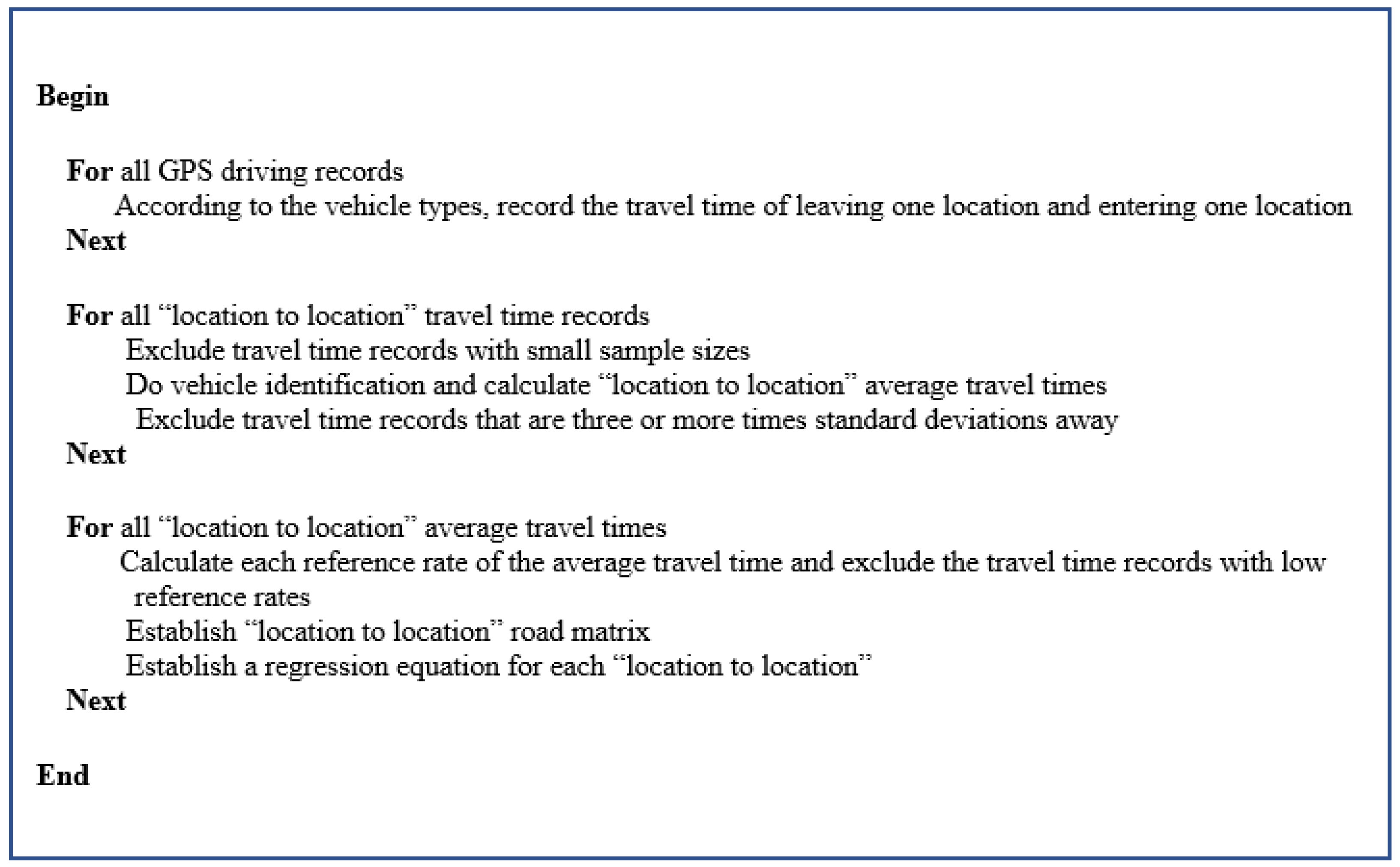
In a normal distribution curve table, the probability of a data point’s Z-score being ≤3 is 95.7%, and the probability of it being >3 is 4.3%. Therefore, in this study, data points with a Z-score of >3 were considered outliers and did not account for more than 4.3% of the total data. The average and standard deviation of the travel times between a pair of departure and arrival locations were calculated, with the data points that were three or more standard deviations away from the average being excluded. The average of the remaining data was then calculated and used as the average travel time between the pair of departure and arrival locations. The data are stored in the MS SQL database using T-SQL for computing which can ignore the process of importing data and reduce the time. A Pseudocode is shown in Figure 3.

Following the aforementioned procedures, we could obtain the average travel time between two points for which historical travel data were available. However, not all pairs of locations had direct travels between them, and for some locations, the number of direct travels was low. For these locations, the average calculation was not conducted because sample size reflects the quality of the result, with a larger sample indicating a higher level of representativeness of the obtained result. A small sample would possibly fail to reflect the actual travel time under regular travel conditions. To ensure the quality of our results, travel history with an inadequate sample size was excluded.

Before proceeding with this study, the original electronic maps used by the fleet estimated the travel time between two locations by planning the shortest route and the static predicted travel time, without considering the traffic conditions in different periods or peak and off-peak travel hours. Since the travel time is obtained from the electronic map planning route, the data source is the determined road length and speed limit, which should be highly representative in theory. However, additional verification was required if this study’s estimated results differed considerably from the estimations by the electronic maps. A reference ratio is the percent ratio of the sample size to the difference between the estimated and electronic map data. The number of samples has a positive relationship with the reference rate, while the difference between the predicted results and the electronic map’s estimations has a negative relationship with the reference rate. First, the predicted travel time is obtained from the model and the ratio of the difference between the travel time of the original map and the travel time of the original map. Then, the reference rate is obtained by (number of samples/time difference) × 100%. The lower reference rates will be excluded and not used, to confirm that the quality of the statistical results is sufficient to replace the prediction results of the original map. For example, if there is a group of data with a sample size of 17, the average travel time obtained by this study model is 3270, and the travel time predicted by the map is 2796, the time difference is (3270 − 2796)/2796 = 16.9, and the reference rate is 17/16.9, which is about 100%. The equation of reference rate is shown in (3).

$$reference rate=\frac{n_{sample}}{(\frac{\left|t_{avg}-t_{map}\right|}{t_{map}})}\ast 100\%$$

(3)

$$n_{sample}=Number of samples$$

$$t_{avg}=average travel time$$

$$t_{map}=Travel time on the map$$

To prevent the lack of historical travel data for some location pairs from undermining the quality of dispatch scheduling, this study filled the missing data by using the established intervallic road networks as training data for machine learning and constructing a nonlinear regression equation. Since the distribution tasks span the peak and off-peak time all day, it is usually a nonlinear regression, which can be a parabolic function. The regression equation is shown in (4).

$$y=a{x}^3+b{x}^2+cx+\epsilon$$

(4)

Finally, this study validated the prediction model with a 6 month travel time record. If the MAPE performance is small, it means that the proposed model can be used in the logistics fleet study. Figure 4 depicts this study’s data processing procedure.

4. Results

The target logistics fleet of this study comprised nearly 1000 vehicles, which generated a total of 65,249,808 travel records from April 2021 to March 2022 (

Table 1. Example of a track log.

License Plate	Status	Time	Speed (km/h)	Location
Car01	Driving	17 March 2022 08:07:50	7	Taoyuan Warehouse
Car01	Leaving the geofence	17 March 2022 08:08:20	40	Section 1, Fenliao Road, Linkou District, New Taipei City (City Road No. 108)
Car01	Driving	17 March 2022 08:08:20	40	Section 1, Fenliao Road, Linkou District, New Taipei City (City Road No. 108)
Car01	Driving	17 March 2022 08:08:50	41	Section 1, Fenliao Road, Linkou District, New Taipei City (City Road No. 108)
		⋮
Car01	Temporarily parked outside	17 March 2022 08:19:50	0	Section 1, Wenhuasan Road, Linkou District, New Taipei City (Country Road Bei No.75)
Car01	Driving	17 March 2022 08:20:20	16	Section 1, Wenhuasan Road, Linkou District, New Taipei City (Country Road Bei No.75)
Car01	Driving	17 March 2022 08:20:50	38	Section 1, Wenhuasan Road, Linkou District, New Taipei City (Country Road Bei No.75)
Car01	Parked in the geofence	17 March 2022 08:21:20	4	Linkou First Store, Linkou District, New Taipei City

). The first record suggested that Car01 was at Taoyuan Warehouse, and the second record indicated that Car01 was on a road. Therefore, the time mentioned in the second record was considered as Car01’s departure time from the warehouse. The second last record indicates that Car01 was on a road, and the last record suggests that Car01 was at Linkou First Store. Accordingly, the time mentioned in the last record was considered Car01’s arrival time at the aforementioned store.

A travel time record was obtained according to Car01’s departure times from Taoyuan Warehouse and arrival times at Linkou First Store (Table 1). By using the aforementioned procedure, we calculated the travel time between any two points for all vehicles in the fleet by using their 65 million records from 2022 and obtained 3,794,744 travel time records (

Table 2. Example of a travel time record.

Origin	Destination	Departure Time	Arrival Time	Travel Time (s)	Period Number
Taoyuan Warehouse	Linkou First Store	17 March 2021 08:08:20.000	17 March 2021 08:21:20.000	780	8
Tucheng Jinfu Store	Tucheng Industrial Store	17 March 2021 20:59:15.000	17 March 2021 21:00:17.000	62	20
		⋮
Xinpu Xinwhenshan Store	Xinpu Shuiyuan Store	17 March 2021 00:26:08.000	17 March 2021 00:32:43.000	395	0
Xinpu Shuiyuan Store	Xinpu Changmao Store	17 March 2021 00:36:08.000	17 March 2021 00:37:31.000	83	0

). The first travel time record (travel time of 780 s) was obtained for the travel data from Taoyuan Warehouse (departed at 08:08:20 on 17 March 2022) to Linkou First Store (arrived at 08:21:20 on 17 March 2022), as presented in Table 1. Because all the vehicles traveling from Taoyuan Warehouse to Linkou First Store were included in the calculation, the vehicle numbers were not recorded in the travel time records.

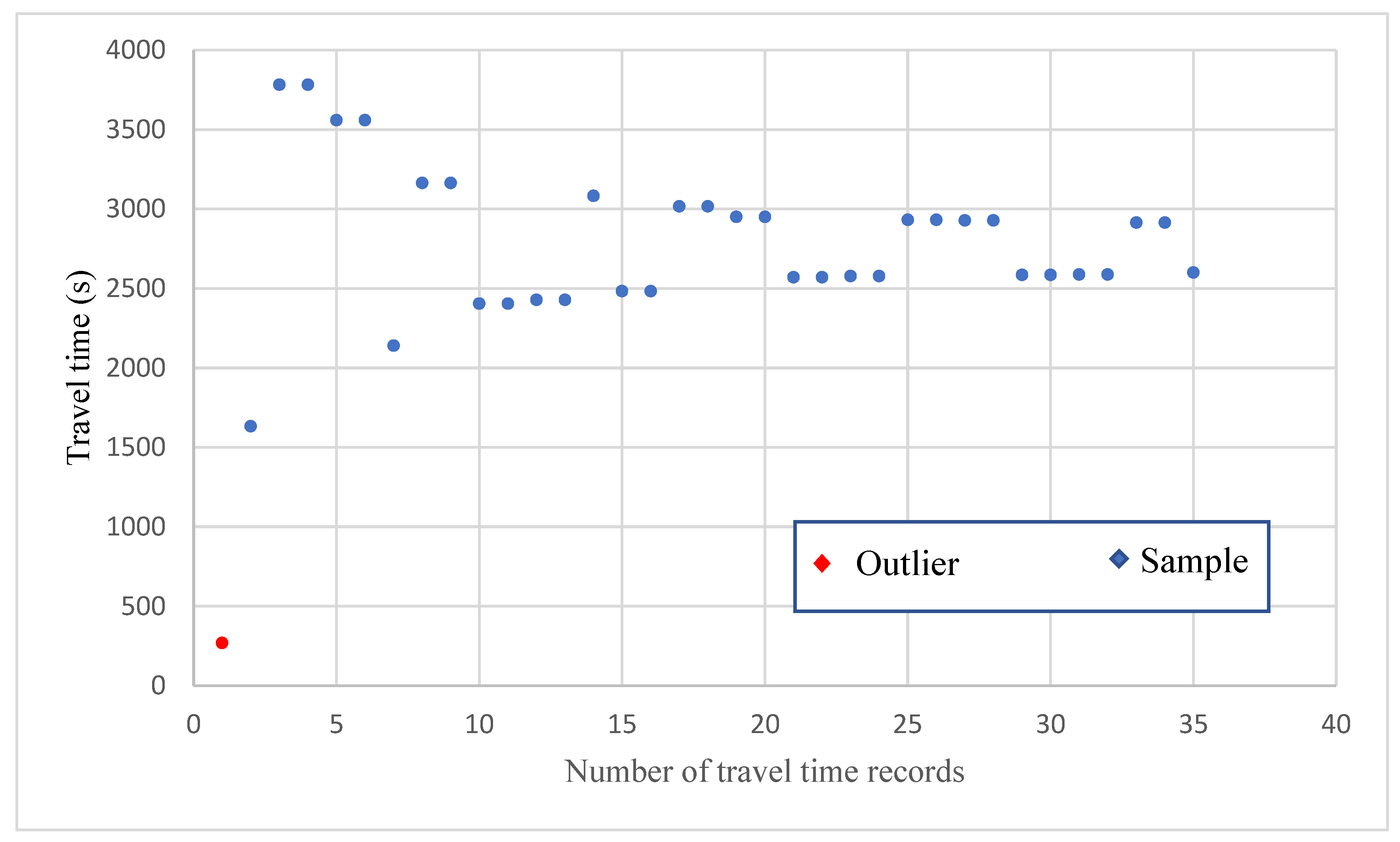
The travel time records were then grouped by departure location, arrival location, and departure period. Consider the combination of Kaohsiung Warehouse and Zhutian First Store as an example. A total of 477 travel records for departure were found between these two points in period 6 (6:00–6:59;

Table 3. Travel time records for travel from Kaohsiung Warehouse to Zhutian First Store in period 6 (6:00–6:59) (Time unit: seconds, including outliers).

Origin	Destination	Departure Time	Arrival Time	Travel Time (s)	Period Number	Average Travel Time	Fold Change
Kaohsiung Warehouse	Zhutian First Store	24 September 2021 6:50	24 September 2021 8:26	5752	6	2668.5	6.9
Kaohsiung Warehouse	Zhutian First Store	1 August 2021 6:34	1 August 2021 8:04	5752	6	2668.5	6.9
Kaohsiung Warehouse	Zhutian First Store	5 July 2021 6:35	5 July 2021 7:31	5356	6	2668.5	6.0
			⋮
Kaohsiung Warehouse	Zhutian First Store	4 July 2021 6:42	4 July 2021 7:21	2236	6	2668.5	1.0
Kaohsiung Warehouse	Zhutian First Store	12 September 2021 6:32	12 September 2021 7:22	3058	6	2668.5	0.9
Kaohsiung Warehouse	Zhutian First Store	4 September 2021 6:22	4 September 2021 7:01	3058	6	2668.5	0.9

). Figure 5 presents the data distribution of these records, with the vertical and horizontal axes representing the travel time (seconds) and number of records, respectively. Most of the travel times were concentrated around 2600 s.

Table 4. Travel time records for travel from Kaohsiung Warehouse to Zhutian First Store in period 7 (7:00–7:59) (Time unit: seconds, including outliers).

Origin	Destination	Departure Time	Arrival Time	Travel Time (s)	Period Number	Average Travel Time	Fold Change
Kaohsiung Warehouse	Zhutian First Store	12 May 2021 07:27:57.000	12 May 2021 07:32:25.000	268	7	2728	4.05
Kaohsiung Warehouse	Zhutian First Store	15 April 2021 07:34:24.000	15 April 2021 08:01:36.000	1632	7	2728	1.80
Kaohsiung Warehouse	Zhutian First Store	2 April 2021 07:41:03.000	2 April 2021 08:44:05.000	3782	7	2728	1.74
			⋮
Kaohsiung Warehouse	Zhutian First Store	31 July 2021 07:04:56.000	31 July 2021 07:45:24.000	3163	7	2728	0.72
Kaohsiung Warehouse	Zhutian First Store	10 September 2021 07:02:06.000	10 September 2021 07:53:28.000	3163	7	2728	0.72
Kaohsiung Warehouse	Zhutian First Store	28 May 2021 07:14:59.000	28 May 2021 07:56:22.000	2404	7	2728	0.53

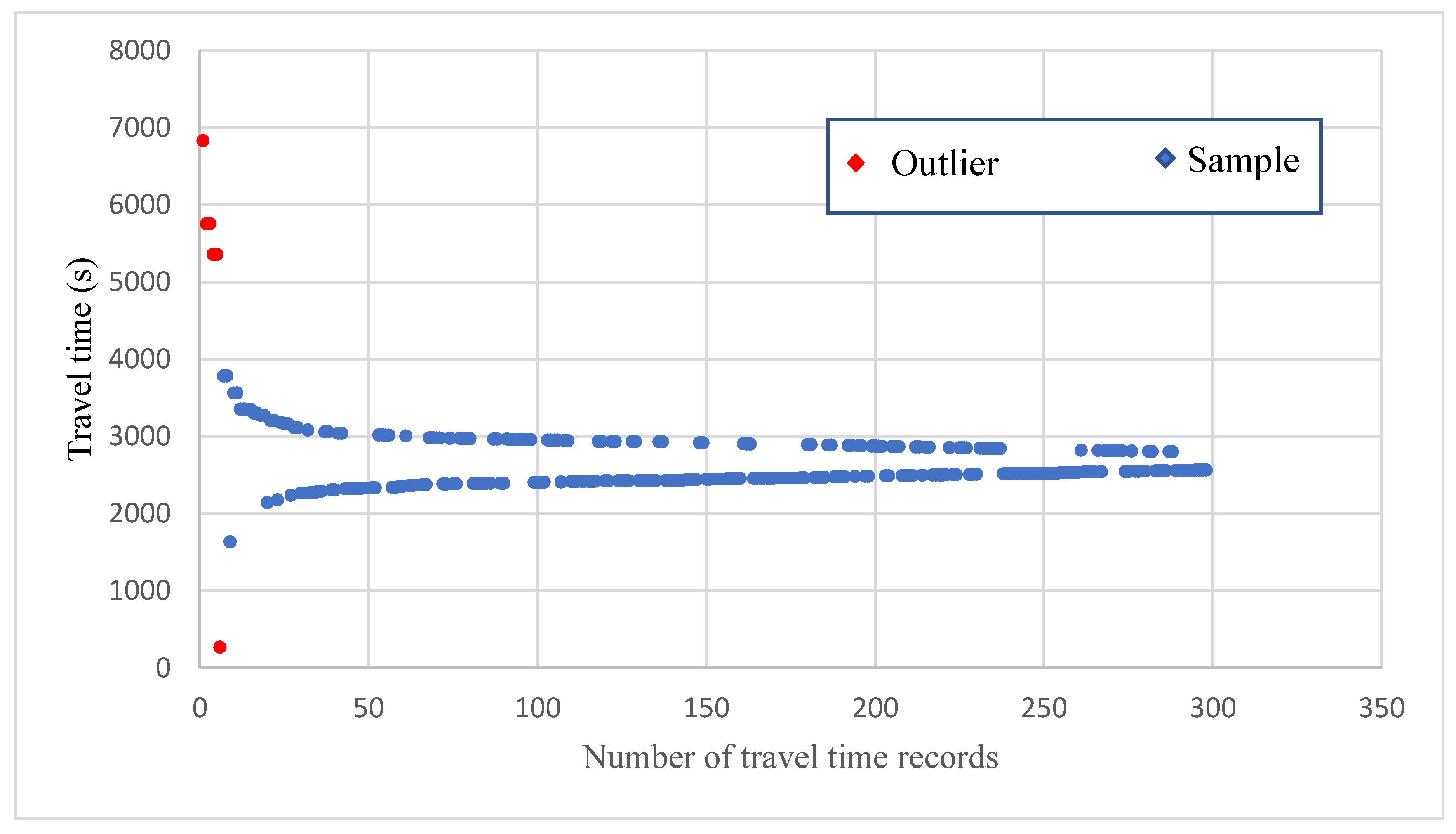
presents the travel time records for departure in period 7, and the data distribution of these records is shown in Figure 6. In total, 298 daily travel time records were collected (

Table 5. Daily travel time records for travel from Kaohsiung Warehouse to Zhutian First Store (Time unit: seconds, including outliers).

Origin	Destination	Departure Time	Arrival Time	Travel Time (s)	Average Travel Time	Fold Change
Kaohsiung Warehouse	Zhutian First Store	11 June 2021 5:36	11 June 2021 7:30	6830	2690	7.9
Kaohsiung Warehouse	Zhutian First Store	24 September 2021 6:50	24 September 2021 8:26	5752	2690	5.8
Kaohsiung Warehouse	Zhutian First Store	1 August 2021 6:34	1 August 2021 8:04	5752	2690	5.8
Kaohsiung Warehouse	Zhutian First Store	12 May 2021 7:27	12 May 2021 7:32	5356	2690	5.1
			⋮
Kaohsiung Warehouse	Zhutian First Store	19 December 2021 6:31	19 December 2021 7:08	3297	2690	1.2
Kaohsiung Warehouse	Zhutian First Store	24 November 2021 6:42	24 November 2021 7:34	3274	2690	1.1
Kaohsiung Warehouse	Zhutian First Store	11 July 2021 6:45	11 July 2021 7:22	3274	2690	1.1
Kaohsiung Warehouse	Zhutian First Store	10 September 2021 7:02	10 September 2021 7:53	2140	2690	1.0

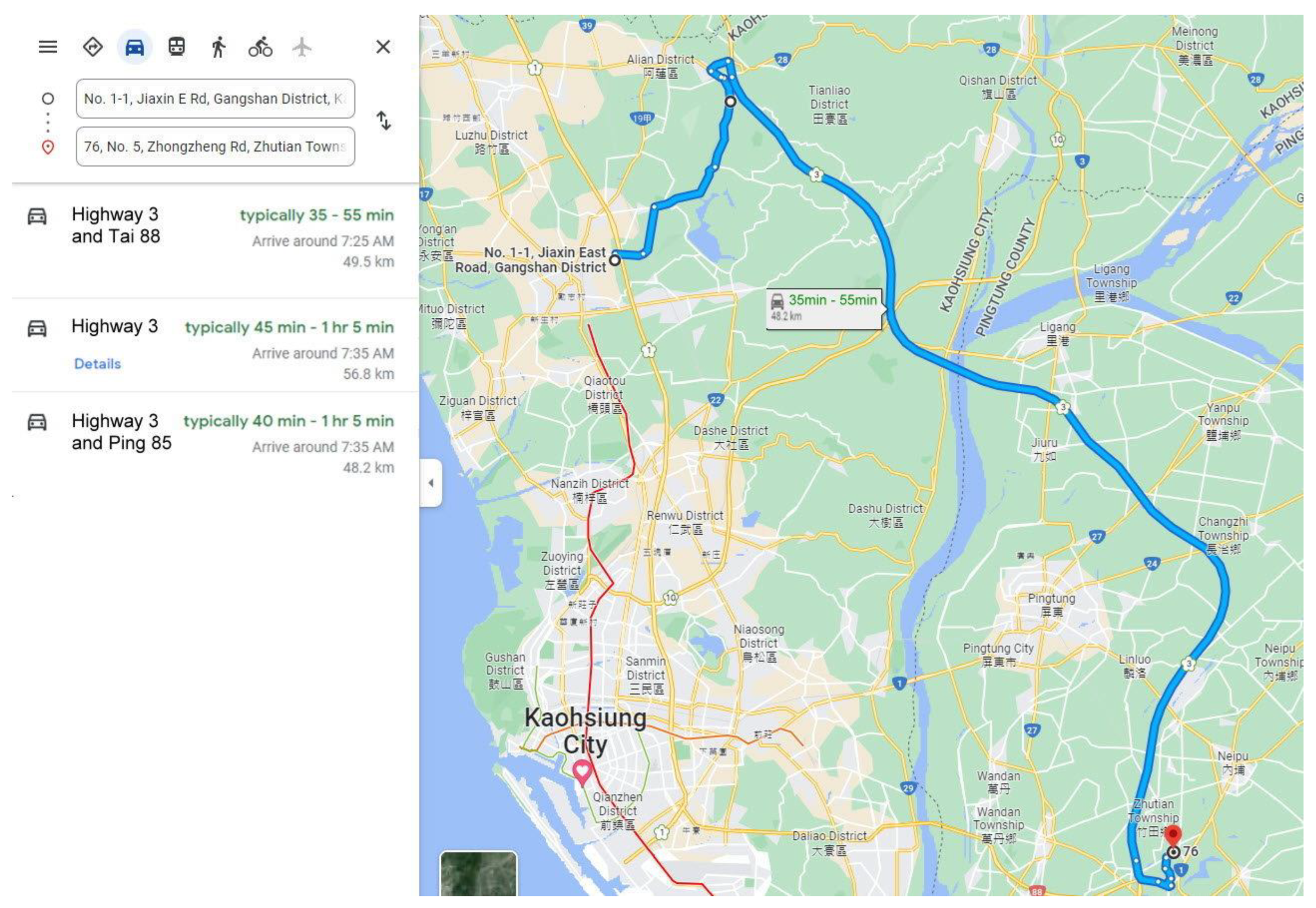
), and their data distribution is displayed in Figure 7. The travel times were mostly concentrated around 2600 s, and the shortest and longest travel times were within 1000 and over 7000 s, respectively. On Google Maps, the estimated travel time for departure at 06:30 on the next day between the aforementioned locations was 35–55 min (2100–3300 s) (Figure 8), and this range covers the majority of daily travel times obtained in this study.

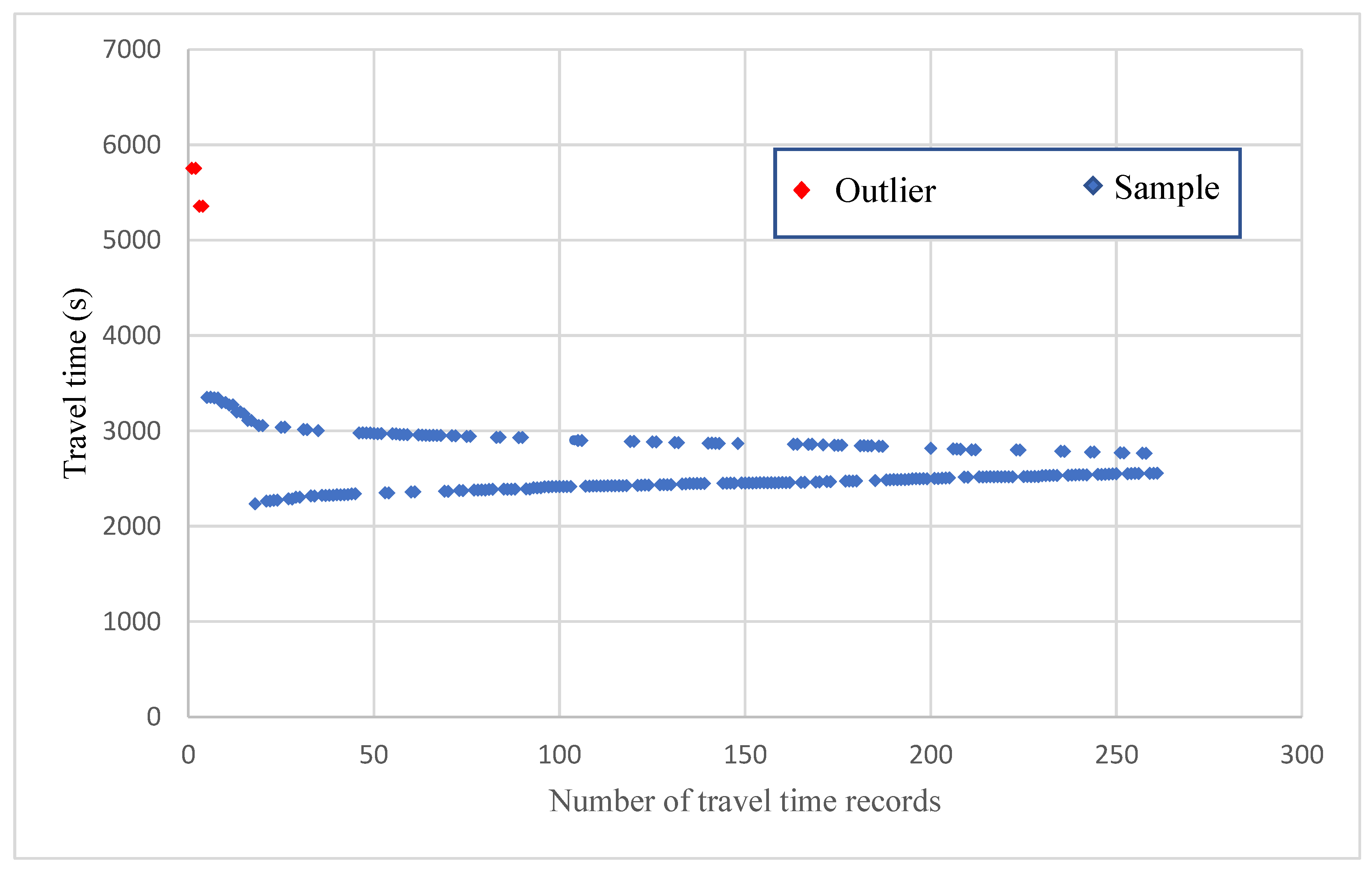
Travel time records that deviated considerably from the average were considered outliers and thus excluded from the analyses because they would undermine the accuracy of our results.

Consider the example of traveling from Kaohsiung Warehouse to Zhutian First Store. For this route, the number of travel time records collected in period 6 (06:00–06:59) was 261. The average and standard deviation values of these records were 2688 and 455 s, respectively. Four travel time values were longer than three standard deviations from the average travel time, as presented in Table 3. Therefore, these four outliers were removed, and the average travel time was recalculated to be 2623 s or approximately 44 min. For the aforementioned route, the number of travel time records collected in period 7 (07:00–07:59) was 35. The average and standard deviation values of these records were 2728 and 607 s, respectively. One travel time value was longer than three standard deviations from the average travel time, as presented in Table 4; therefore, this value was removed. The average travel time recalculated using the remaining 34 records was 2800 s or approximately 47 min.

With regard to daily travel records, 298 travel time records were obtained for the route from Kaohsiung Warehouse to Zhutian First Store. The average travel time was 2690 s, the standard deviation was 525 s, and six records were three or more standard deviations away from the average (Table 5). These six records were excluded, and the average was recalculated to be 2645 s or approximately 44 min. On Google Maps, the estimated travel time for the aforementioned journey for departure at 6:30 on the next day was 35–55 min, and this range covered the average values obtained in this study when considering and not considering the outliers (Figure 7).

A total of 0.4% and 1.7% of the hourly and daily data, respectively, were defined as outliers and removed from subsequent analyses. The remaining data were then subjected to another check based on two factors—sample size and reference ratio—to reconfirm their suitability for inclusion in the subsequent analyses.

A total of 3,779,725 point-to-point hourly travel time records were obtained after the outliers were removed. These data were grouped by departure location, arrival location, and departure period, and 199,872 rows of data were obtained. Each row of data represents a specific combination of departure point, arrival point, and departure period (hereafter referred to as the “intervallic combination”). The intervallic combination reveals the average travel time—which was calculated using all historical travel records along a route in a given period and excluding outliers—and the sample size, which is the number of travel records included in the average calculation. Intervallic combinations with a sample size smaller than 1% of the largest sample in a group were excluded for their under-representativeness. For example, when the largest sample size was 522 records and thus 1% of the sample size was approximately five records, 124,353 intervallic combinations with less than five travel records were excluded, and 75,519 intervallic combinations remained. For the daily data, each row of data represents a specific combination of departure point and arrival point (hereafter referred to as the “daily combination”) and reveals the daily average travel time and sample size for this combination. Among all the daily combinations, the largest sample size was 1587 travel records; thus, 56,318 daily combinations with a sample size of less than 16 (approximately 1% of the largest sample size) were excluded, and the total daily sample size decreased from 77,765 to 21,447 combinations. Of these 21,447 combinations, 117 had the same travel times as those estimated by the fleet’s electronic map. These 117 combinations were also excluded, and the total daily sample size decreased further to 21,330 combinations.

After combinations with an inadequate sample size and with the same travel times as those estimated by the fleet’s electronic map were excluded, Equation (1) was used to calculate the reference ratio for the remaining combinations (

Table 6. Some calculated reference ratio values (Time unit: seconds).

Origin	Destination	Travel Time (s)	Intervallic Travel Time (s)	Period Number	Time Estimated Using Electronic Maps (s)	Sample Size	Time Difference	Reference Ratio
Daxi Warehouse	Zhonghe Shiji Store	3415	3270	7	2796	17	17.0%	100.3%
Zhonghe Zhenxin Store	Daxi Warehouse	3158	3520	18	2796	26	25.9%	100.4%
Emei Taisanxian Store	Nanzhuang Guihuayuan Store	1690	1600	8	1608	271	0.5%	54471.0%
Taichung Fuda Store	Taichung Warehouse	1588	1682	23	2796	40	39.8%	100.4%
			⋮
Yangmei Station Store	Yangmei Beidu Store	563	578	13	386	50	49.6%	100.7%
Zhongli Yuanxing Store	Zhongli Longgang Store	427	487	12	566	14	14.0%	100.3%
Meihua Store	Zhishan Store	295	286	9	185	55	54.9%	100.2%
Tainan Changxi Store	Tainan Beizhou Store	280	343	16	258	33	32.9%	100.2%

). A higher reference ratio is associated with a larger sample and a smaller travel time difference. Given the absence of a standard or preestablished threshold for the reference ratio, this study set a threshold of 20%. Specifically, combinations whose reference ratios were in the bottom 20% were excluded. For hourly travel time data, the sample size was decreased from 75,289 to 60,344 combinations (reference ratio in the 80th percentile = 8.3%). For daily travel time data, the sample size was decreased from 21,330 to 17,066 combinations (reference ratio in the 80th percentile = 32.2%).

Different quantities of statistical data were acquired after different stages of data processing.

Table 7. Variations in the number of records in the data processing stages (Time unit: seconds).

Type of Records	Number of Original GPS Tracks	Number of Travel Time Records	Number of Records Obtained after Removing Outliers	Number of Average Time Records	Number of Records with a Sample Size Higher than the Threshold	Number of Records with a Reference Ratio Higher than the Threshold
Intervallic records	65,249,808	3,794,744	3,779,725	199,872	75,289	60,344
Daily records			3,728,516	77,765	21,330	17,066

presents the variations in the number of records in the data processing stages.

From the 60,344 intervallic combinations and 17,066 daily combinations obtained after data exclusion, the travel times of 16 random intervallic combinations and 16 random daily combinations were compared with the corresponding travel times estimated using Google Maps (

Table 8. Intervallic travel time, daily travel time, and travel time estimated using Google Maps.

Origin	Destination	Daily Travel Time (s)	Period Number	Intervallic Travel Time (s)	Travel Time Estimated Using Google Maps (s)
Daxi Warehouse	Zhonghe Shiji Store	3415	7	3270	1800~4200
Zhonghe Zhenxin Store	Daxi Warehouse	3158	18	3520	2400~4500
Emei Taisanxian Store	Nanzhuang Guihuayuan Store	1690	8	1600	1440~2100
Taichung Fuda Store	Taichung Warehouse	1588	23	1682	1080~1560
		⋮
Yangmei Station Store	Yangmei Beidu Store	563	13	578	480~960
Zhongli Yuanxing Store	Zhongli Longgang Store	427	12	487	300~720
Meihua Store	Zhishan Store	295	9	286	240~480
Tainan Changxi Store	Tainan Beizhou Store	280	16	343	240~420

). Substantial differences were noted between the intervallic and daily travel times. All of this study’s daily travel times fell within the corresponding estimated travel time ranges for next-day departure on Google Maps.

An intervallic combination with a small sample of travel records hinders accurate travel time estimation by dispatchers in the scheduling of future delivery along a certain route in a specific period. Therefore, in this study, the intervallic travel time records were employed in machine learning to generate estimated travel times for other periods. Consider the route from Guanshan Minzu Store to Taitung Luye Store (Table 8) as an example.

Table 9. Intervallic travel time from Guanshan Minzu Store to Taitung Luye Store.

Origin	Destination	Period Number	Intervallic Travel Time (s)
Guanshan Minzu Store	Taitung Luye Store	2	1497
Guanshan Minzu Store	Taitung Luye Store	3	1493
Guanshan Minzu Store	Taitung Luye Store	4	1608
Guanshan Minzu Store	Taitung Luye Store	5	1690
Guanshan Minzu Store	Taitung Luye Store	6	1553
Guanshan Minzu Store	Taitung Luye Store	9	1467
Guanshan Minzu Store	Taitung Luye Store	10	1402
Guanshan Minzu Store	Taitung Luye Store	11	1394
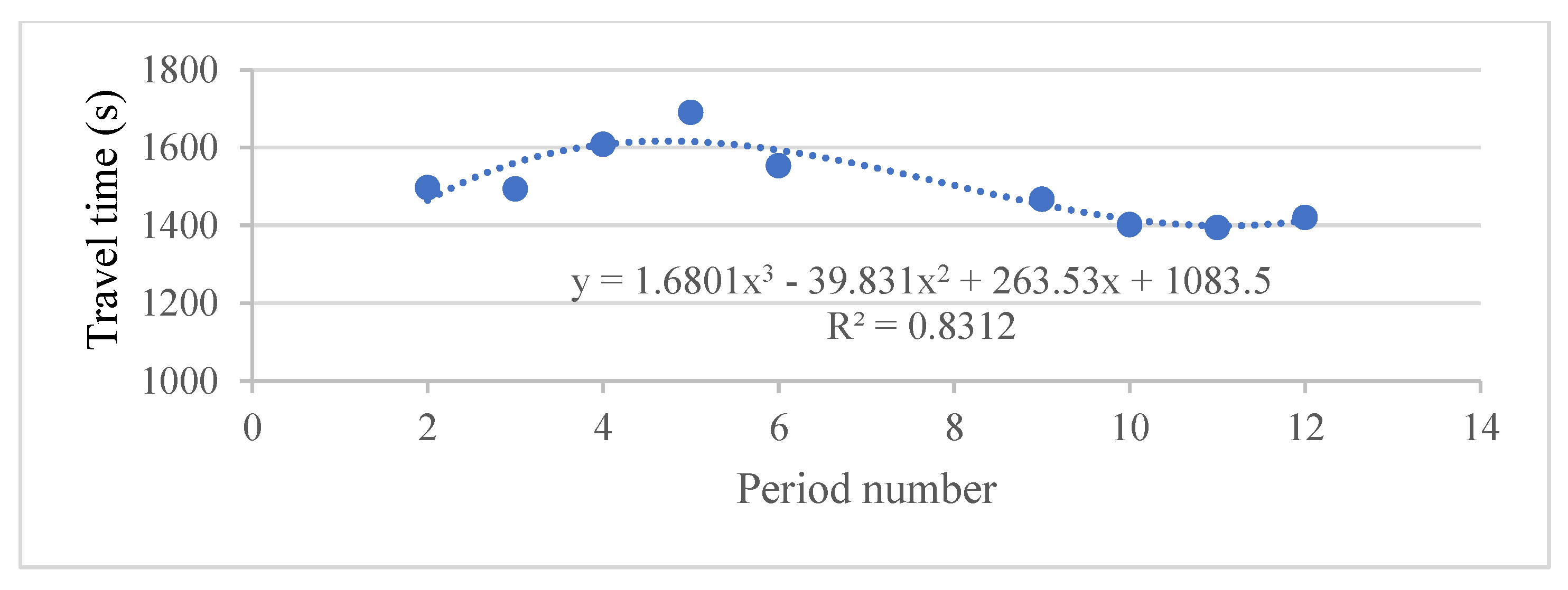
Guanshan Minzu Store	Taitung Luye Store	12	1420

reveals the hourly travel times for this route and indicates that the average travel time data were available only for periods 2–6 and periods 9–12 but not for other periods. These available data were used to construct a polynomial regression equation: y = 1.6801x³ − 39.831x² + 263.53x + 1083.5, where x denotes the period, and y is the travel time (Figure 9).

If a dispatcher must schedule delivery vehicles to travel from Guanshan Minzu Store to Taitung Luye Store in a period for which average travel time data are unavailable, we can use the aforementioned equation to estimate the travel time. In Table 9, there is no average travel time between period 7 and period 8. After applying the regression equation, the predicted travel time in period 7 is 1552.76 s, and the relevant calculation is presented in Equation (5). The predicted travel time in period 8 is 1502.76 s, and the relevant calculation is presented in Equation (6).

$${1.6801\left(7\right)}^3-{39.831\left(7\right)}^2+263.53\left(7\right)+1083.5=1552.76$$

(5)

$${1.6801\left(8\right)}^3-{39.831\left(8\right)}^2+263.53\left(8\right)+1083.5=1502.76$$

(6)

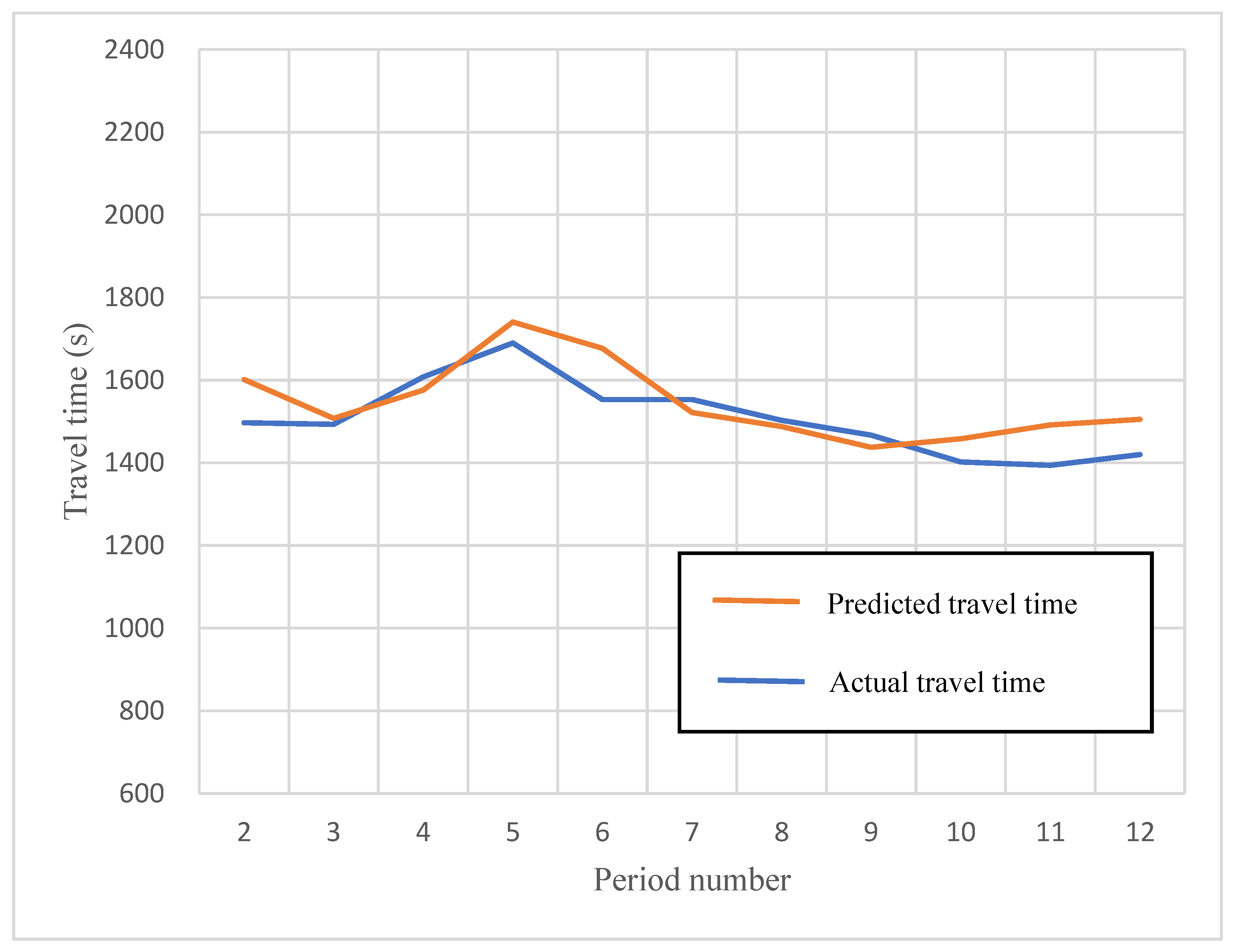
The aforementioned model for predicting travel time used the data between April 2021 and March 2022 for one year, which are used as the training data. The data between April 2022 and September 2022 for six months are used as the validation data. Compare the MAPE of the same locations of travel time to validate the model established in this study. From Guanshan Minzu Store to Taidong Luyedian as an example in aforementioned Table 9, the model in this study which obtained the travel time from 2 to 12 with the data between April 2022 and September 2022 for six months using MAPE to obtain the result is 2.52%, which represents the model has 2.52% error using machine learning in this study. The formula of MAPE is shown in Equation (7), and the results are shown in

Table 10. Validation result of travel time.

Origin	Destination	Period Number	Predicted Travel Time (s)	Actual Travel Time (s)
Guanshan Minzu Store	Taitung Luye Store	2	1497	1602
Guanshan Minzu Store	Taitung Luye Store	3	1493	1508
Guanshan Minzu Store	Taitung Luye Store	4	1608	1576
Guanshan Minzu Store	Taitung Luye Store	5	1690	1741
Guanshan Minzu Store	Taitung Luye Store	6	1553	1677
Guanshan Minzu Store	Taitung Luye Store	7	1553	1522
Guanshan Minzu Store	Taitung Luye Store	8	1503	1488
Guanshan Minzu Store	Taitung Luye Store	9	1467	1438
Guanshan Minzu Store	Taitung Luye Store	10	1402	1458
Guanshan Minzu Store	Taitung Luye Store	11	1394	1492
Guanshan Minzu Store	Taitung Luye Store	12	1420	1505

. The curves of the predicted and actual travel time are shown in Figure 10.

$$\mathrm{M}\mathrm{A}\mathrm{P}\mathrm{E}=\frac{100\%}{n}{\sum }_{i=1}^n\left|\frac{\widehat{y_i}-y_i}{y_i}\right|\hspace{1em}\hspace{1em}\hspace{1em}n=11$$

(7)

5. Discussion

The logistics operation of convenience stores is limited by the location of the store and different goods must be delivered at the designated time. When arranging the route, the dispatchers cannot choose the roads or periods without traffic jams. If the travel time between locations can be predicted, it can be useful for route arrangement and unloading preparation operations. Thus, this study used GIS spatial technology to obtain the travel time records from the GPS driving records and then used machine learning to perform the average travel time. This study also added standard deviation, sample, and reference ratio we designed to filter the data to ensure the quality of the prediction results. The nonlinear regression equation is used to supplement the period of unavailable data, and the actual driving time is used to validate the predicted model. This study estimated travel times between two locations at different hours, which are particularly helpful for scheduling future delivery tasks. In the proposed approach, the total time required to complete deliveries at convenience stores along a route is calculated by summing the travel time between convenience stores and the unloading time at each store. The result is then used to schedule the following delivery route. The proposed method also reveals estimated arrival times, the knowledge of which allows convenience stores to make room in advance for delivery vehicles to park, unload, and complete other work. However, additional data might be required for intervallic records. The fleet investigated in this study did not use GPS on their vehicles until 2021; therefore, the study data (approximately 65 million travel records) were collected from April 2021 to March 2022. Future studies can expand their samples to enhance the representativeness of their results.

This study focused on travel time discussion. The task clustering and travel route (arrival order) are excluded from this article. The future study will explore two crucial topics in depth in a separate study.

In practice, the arrival time might vary because of weather conditions, traffic, and accidents. The influence of these unexpected events on travel times was not considered in this study. Future research can develop approaches to recommend alternative routes that minimize the additional travel time required in case of unexpected events.

According to the results of this study, each combination of departure and arrival points usually had a few periods of the day in which the numbers of journeys were distinctly higher than those during the other periods of the day, and each period usually lasted for a few hours. For example, if the journeys between a specific combination of departure and arrival points are concentrated around two periods, namely the most common time 06:00–08:00 in the morning and the other time 13:00–15:00 in the afternoon, the travel times during the same period can be considered the same as each other but different from those during the other period. Accordingly, future research with larger samples can use 3 h as a time unit to simplify the relevant calculations.

This study examined the travel times between warehouses and convenience stores or between convenience stores and thus is applicable to travel time estimation between fixed departure and arrival points. Future studies can expand on this study to estimate travel times between a warehouse and any given point for application in home delivery fleets. Studies can also divide a map into different areas, with each area being represented by a crossroad, and then identify the area that the target location belongs to so that they can estimate the travel time from the departure point to the corresponding crossroad and then sum it with the estimated travel time from the crossroad to the target location for obtaining the total travel time.

To estimate the travel times in periods for which historical travel data were unavailable, this study used the travel times estimated for other periods to perform machine learning and establish a nonlinear regression equation capable of generating estimated travel times for the periods with no data.

This study employed GPS data collected from fleet vehicles rather than the average driving speed data for each road or historical data because company policies, driver habits, vehicle performance, and procedures might vary across fleets. Thus, the average driving speed on each road might vary across fleets. Based on the actual operating experience and the normal distribution principle of Statistics, this study filtered the outliers. For future research, we will strengthen data collection from GPS driving records and deeply discuss the causes of these outliers and their impact on the prediction model. By collecting GPS records for a specific fleet, this study obtained results that accurately reflected the fleet’s operations. However, the generalizability of the results of this study to other fleets requires further verification.

6. Conclusions

In this study, the travel time prediction model established by the machine learning algorithm used three or more standard deviations away, sample, and reference ratio we designed to filter unreasonable data to avoid error accumulation. For the GPS driving records that were not collected during the periods, this study used the nonlinear regression equation to obtain predicted data to fill the gap in the original data sources. This study used machine learning based on the 12-month historical driving records of the target logistics fleet and then validate the 6-month driving records. Giving Guanshan Minzu Store to Taitung Luye Store as an example, using the driving records for the machine learning model between April 2021 and March 2022 and the actual average travel time collected between April 2022 and September 2022 for validation, the MAPE is only 2.52%. Thus, the prediction model in this study can have a performance of more than 97%. Based on historical data and the proposed machine learning algorithm can obtain estimated travel times for their scheduling of future delivery tasks and make the predetermined schedule more efficient.

Based on the results of this study, it can be known that the travel time between the same two locations has differences at different periods, which is caused by the road conditions, traffic flow, and environmental conditions between the two locations. Through the prediction model established in this study, the managers of convenience stores should be able to conceive and schedule future deliveries, they should try to make use of the short travel time to achieve logistics transportation operations to reduce the traffic impact on roads and communities, reduce the operation time, reduce the operation cost of the fleet, and further improve the operational efficiency of logistics transportation.