Article

Synchronization, Control and Data Assimilation of the Lorenz System

by
Franco Bagnoli
1,2,*,† and
Michele Baia
1,2,†
1
Department of Physics and Astronomy and CSDC, University of Florence, Via G. Sansone 1, 50019 Sesto Fiorentino, Italy
2
INFN, Sect. Florence, Via G. Sansone 1, 50019 Sesto Fiorentino, Italy
*
Author to whom correspondence should be addressed.
These authors contributed equally to this work.
Algorithms 2023, 16(4), 213; https://doi.org/10.3390/a16040213
Submission received: 16 March 2023 / Revised: 10 April 2023 / Accepted: 17 April 2023 / Published: 19 April 2023
(This article belongs to the Special Issue Algorithms for Natural Computing Models)

Abstract

:
We explore several aspects of replica synchronization with the goal of retrieving the values of parameters applied to the Lorenz system. The idea is to establish a computer replica (slave) of a natural system (master, simulated in this paper), and exploit the fact that the slave synchronizes with the master only if they evolve with the same parameters. As a byproduct, in the synchronized phase, the state variables of the slave and those of the master are the same, thus allowing us to perform measurements that would be impossible in the real system. We review some aspects of master–slave synchronization using a subset of variables with intermittent coupling. We show how synchronization can be achieved when some of the state variables are available for direct measurement using a simulated annealing approach, and also when they are accessible only through a scalar function, using a pruned-enriching ensemble approach, similar to genetic algorithms without cross-over. We also explore the case of exploiting the “gene exchange” option among members of the ensemble.

1. Introduction

There are many cases in which one is interested in forecasting the behavior of a chaotic system; an emblematic example is meteorology. The main obstacle is, of course, that in chaotic systems, by definition, a small uncertainty can amplify exponentially over time [1]. Moreover, even if one assumes that a computational model of a natural, chaotic system is a good model, the exact values of parameters are needed to ensure a faithful representation of dynamics.
Schematically, one can assume that the natural, or target, system is well represented by some dynamical system, possibly with noise. One can measure some quantities of this system, but in general, one is not free to choose which variable (or combination of variables) to measure, nor to perform measurements at any rate.
On the other hand, if one has a good knowledge of the system under investigation, i.e., it can be modeled with good accuracy, then a simulated “replica” of the system can be implemented on a computer. If, moreover, it is possible to know the parameters and the initial state of the original system, in order to keep the replica synchronized to it (when running at the same speed), then the replica can be used to perform measurements that are otherwise impossible, and to obtain accurate forecasting (when run at higher speeds).
In general, the problem of extracting the parameters of a system from a time series of measurements on it is called data assimilation [2].
The problem in data assimilation is that of determining the state and the parameters of the system by minimizing an error function between data measured on the target and the respective data from the simulated system. A similar task is performed by back-propagation techniques in machine learning [3,4].
The goal of this paper is to approach this problem from the point of view of dynamical systems [5]. In this context, the theme of synchronization has been explored [6], but it needs to be extended in order to cover the application field of data assimilation.
The synchronization technique is particularly recommendable when the amount of noise (in the measure and intrinsic to the system) is small, i.e., when the target system can be assumed to be well represented by deterministic dynamics, even if these dynamics are not continuous (as in Cellular Automata [7]).
We shall investigate here the application of synchronization methods to the classic Lorenz system [8]. However, the method can be applied to other chaotic systems and possibly to their implementation in electronic hardware.
The Lorenz system is chosen because, for classical values of parameter, there is only one chaotic attractor. Other systems, such as Chua’s [9,10], may present the coexistence of attractors (hidden attractors) [11,12], which may affect synchronization [13].
Our investigation is carried out considering some synchronization schemes; see Section 2.
We start from the classic Pecora–Carrol master–slave synchronization scheme, recalled in Section 2.1, in which the values of some of the state variables of the master are imposed to the corresponding variables of the slave system. This choice of coupling variables is denoted “coupling direction” in the tangent space of the system.
The synchronization threshold is connected to the value of the conditional Lyapunov exponent [14,15], i.e., the exponential growing rate along the difference space between master and slave, as reported in Section 2.2.
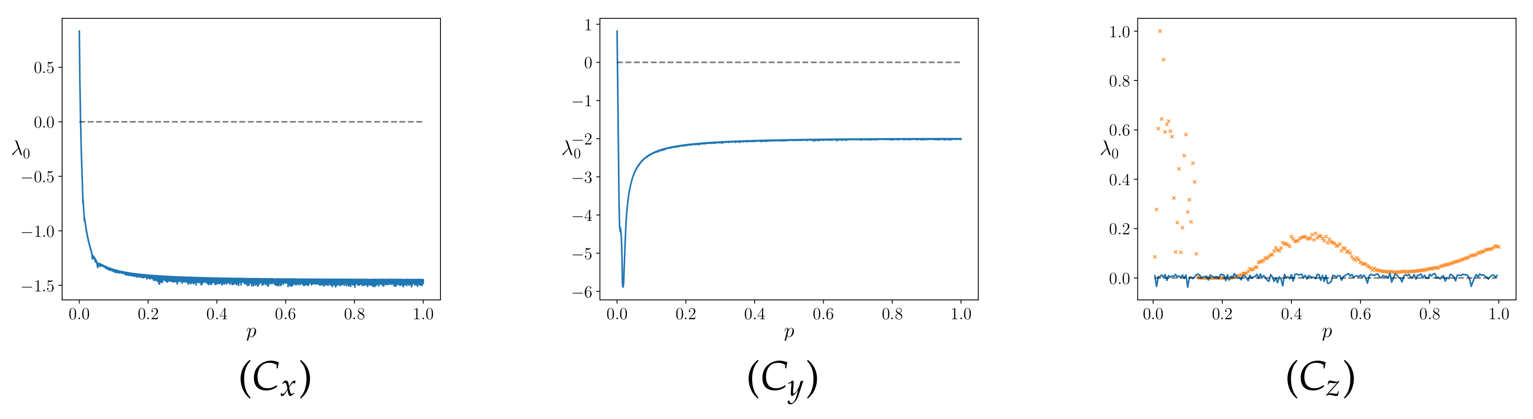
This scheme is then extended to partial synchronization, i.e., to the case in which only a portion of the values of the state variables of the master system signal is fed to the slave, as shown in Section 2.3. We can thus establish the minimum fraction of signal (coupling strength) able to synchronize the two replicas, which depends on the coupling direction.
However, one cannot pretend to be able to perform measurements in continuous time, as achieved in the original synchronization scheme, in which the experimental reference system was a chaotic electronic circuit.
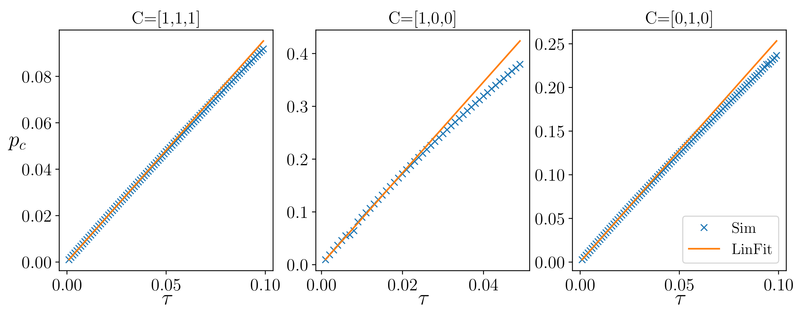
Therefore, we deal with the problem of intermittency, i.e., performing measurements, and consequently applying the synchronization scheme, only at certain time intervals. We show that the synchronization scheme also works for intermittent measurements, provided that the coupling strength is increased, as shown in Section 2.4.
In the case of systems with different parameters, synchronization cannot be complete, and we discuss generalized synchronization; see Section 2.5.
We report some results in Section 3, showing that the distance among systems can be interpreted as a measure of the error and exploited to obtain the “true” values of parameters, using a simulated annealing scheme.
Finally, it may happen that the variables of the systems are not individually accessible to measurements, a situation which prohibits the application of the original method. In this case, one can still exploit schemes inspired by statistical mechanics, such as the pruned and enriching one, simulating an ensemble of systems with different state variables and parameters, selecting the instances with lower rates of error, and cloning them with perturbations. This kind of genetic algorithm is able to approximate the actual values of parameters, as reported in Section 4.
Conclusions are drawn in Section 5.

2. Master–Slave Synchronization

2.1. Pecora–Carrol Synchronization

In 1990, Louis Pecora and Thomas Carrol introduced the idea of master–slave synchronization [14]. They studied simulated systems, such as the Lorenz [8] and Rössler [16] ones, and also experimental electronic circuits [17].
They considered two replicas of the same system with the same parameters. One of the replicas (the master) was left to evolve unperturbed. Some of the state variables of the master replaced the corresponding variables of the slave system, which was therefore no longer autonomous. This topic was further explored in a 2015 paper [15].
In order to explain the main idea of this master–slave (or replica) synchronization, let us consider first a one-dimensional, time-discrete dynamical system, such as, for instance, the logistic map [18]. It is defined by an equation of the kind
x n + 1 = f ( x n ) ,
where n labels the time interval. The usual Lyapunov exponent λ is defined as
λ = lim N n = 1 N log ( f ( x n ) ) ,
where f ( x ) = d f / d x . Let us now introduce a replica X such that
x n + 1 = f ( x n ) ; X n + 1 = ( 1 p ) f ( X n ) + p f ( x n ) ,
where p is the coupling parameter (coupling strength).
For p = 0 , the two maps are uncoupled, and because they are assumed to be chaotic, they generally take different values. For p = 1 , map X immediately synchronizes with map x. There is a critical value p c of the coupling parameter for which the synchronized state is stable, and it is related to the Lyapunov exponent λ ,
p c = 1 exp ( λ ) ,
as can be seen by taking the linearized difference among the maps.
This scenario holds also for higher-dimensional (K) maps, which can be written as
r n + 1 = F ( r n ) ,
where r n denotes the state of the system at iteration n and has K components. The system now has K Lyapunov exponents, of which at least one, λ MAX , is assumed to be positive.
The synchronization procedure in this case is
r n + 1 = F ( r n ) ; R n + 1 = ( I p C ) F ( R n ) + p C F ( r n ) ,
where the coupling is now implemented by means of a diagonal matrix C, with diagonal entries equal to zero or one, defining the coupling directions. In the following, we shall indicate the diagonal of C as C = [ c x , c y , c z ] .
In the case in which C = I , i.e., all entries are mixed with the same proportion, the stability of the synchronized phase is again related to the maximum Lyapunov exponent λ MAX ,
p c = 1 exp ( λ MAX ) ,
because the evolution of an infinitesimal difference among the replicas, δ , is given by
δ n + 1 = ( 1 p ) J ( x ) δ n ,
where J is the Jacobian of F
J i j = F i x j x = x n .
This scheme can be extended to continuous-time systems by replacing the entries from one system in the coupled differential equation, so that
r ˙ = F ( r ) ; R ˙ = ( I p C ) F ( R ) + p C F ( r ) .
where the Lyapunov exponents of the original system are now given by the eigenvalues of the (symmetrized) time-average of Jacobian Λ
Λ = lim t 1 2 t 0 t J ( r ( t ) ) + 0 t J ( r ( t ) ) T .
In practice, however, the differential Equation (10) is implemented as a map by discretizing the time, and therefore, Lyapunov exponents are computed as in the previous case. Using a simple Euler scheme, we have t = n Δ t and r ( t ) = r ( n Δ t ) = r n , and
r n + 1 = r n + F ( r n ) Δ t .
In the tangent space
δ r n + 1 = ( 1 + J ( r n ) Δ t ) δ r n ,
and the maximum Lyapunov exponent λ MAX is
λ MAX = lim n 1 n Δ t n log ( 1 + J ( r n ) Δ t ) lim n 1 n n J ( r n ) .
The average growth of the distance δ r is
δ r ( t ) = δ 0 exp ( λ MAX n Δ t ) = exp ( λ MAX t ) ,
for time intervals such that the linearized approximation is valid.
Notice that, in the continuous-time version, the Jacobian and the Lyapunov exponents are defined in units of the inverse of time.
In this paper, we always use the Euler integration scheme. We checked that other, more sophisticated integration schemes do not qualitatively affect our results.

2.2. Conditional Coupling

In the original Pecora–Carrol implementation [15], the signal from the master is fully extracted, i.e., p = 1 , so that, for the R system, either a component is untouched or it is derived from the replica ( r ).
To be explicit, for the Lorenz system we have
x ˙ = σ ( y x ) , y ˙ = x z + ρ x y , z ˙ = x y β z .
For instance, for a full coupling along the x direction ( C = [ 1 , 0 , 0 ] ), the replica will follow the equation
X = x , Y ˙ = x Z + ρ x Y , Z ˙ = x Y β Z .
It is possible to define the sub-Lyapunov [14] or, better, the conditional Lyapunov exponents [15], by iterating the equation for the difference δ r in the tangent space. For instance, for the Lorenz system coupled along the x direction ( C = [ 1 , 0 , 0 ] ), we have
d d t δ y δ z = 1 x x β · δ y δ z ,
giving two conditional exponents. The system synchronizes if both of them are negative.
In Figure 1, we report the value of the maximum conditional Lyapunov exponent as a function of the coupling strength p for the C x = [ 1 , 0 , 0 ] , C y = [ 0 , 1 , 0 ] , and C z = [ 0 , 0 , 1 ] coupling directions.
As noted also in Ref. [15], the Lorenz system synchronizes if coupled along the x and y directions, but not along the z one, even for p = 1 .
Our observable was the average distance d,
d ( t ) = | | r ( t ) R ( t ) | | = ( x ( t ) X ( t ) ) 2 + ( y ( t ) Y ( t ) ) 2 + ( z ( t ) Z ( t ) ) 2 , d = 1 T 0 T d ( t ) d t ,
computed after a proper transient.
In Figure 2, we show d as a function of the coupling strength p for different coupling directions. For all the simulations, we set σ = 10 , β = 8 / 3 , ρ = 28 , and we use the Euler integration scheme to integrate the equation with a temporal step d t = 10 3 . After a transient time of free evolution, we couple the master and the slave system at every time step. At T = 100 (simulation end time), we compute the distance d between the two systems.

2.3. Partial Conditional Coupling

We can naturally generalize the definition of maximum conditional Lyapunov exponents even when we do not have a full coupling, i.e., p < 1 , by looking for the synchronization threshold p c , for which d ( p ) goes to zero.
From the plots shown in Figure 2, one can see that, for the x and y coupling, there is a well-defined synchronization threshold, similar to that obtained for the uniform coupling. For the z coupling, the maximum Lyapunov exponent is always positive (albeit small), and no synchronization is possible.
This behavior is shown in Figure 1, where we plot the maximum conditional Lyapunov exponent for different coupling strengths p and different coupling directions C. For the z coupling, we also plot the distance d ( p ) for some p (as in Figure 2).
One can also see that, in the unsynchronized phase, the distance d ( p ) exhibits a nonmonotonous behavior, except in the vicinity of the synchronization transitions, as shown in Figure 2. This aspect is analyzed in Section 3.

2.4. Intermittent Synchronization

In real applications, it is generally impossible to obtain a signal from one system and inject it into the replica in a time-continuous way. Pecora and Carrol were able to achieve it using electronic circuits [14], but if one needs to pass through a measurement system, it is expected that this device has a finite bandwidth, i.e., a finite measurement time.
So, the question becomes: is it possible to synchronize two replicas by measuring one quantity only at time intervals τ ?
Numerically, if the equations are integrated using a constant time step Δ t , this means that the replacement or mixing of components is applied every k time steps, so that τ = k Δ t .
For homogeneous coupling ( C = [ 1 , 1 , 1 ] ), the linear analysis simply tells us that (Equation (7))
p c = 1 exp ( λ MAX Δ t · k ) = 1 exp ( λ MAX τ ) ,
i.e., intermittent synchronization is equivalent to standard synchronization for a system with a larger Lyapunov exponent.
Then, for a small τ , we have
p c = λ MAX τ .
This relationship also holds numerically for other coupling directions, as shown in Figure 3. In the figure, we also plot the linear fit obtained using the first 20 points.
The estimated values obtained from the linear fit ( λ fit ), compared with the values ( λ lin ) computed using Equation (21), with p c estimated numerically (Figure 2), are summarized in Table 1.

2.5. Generalized Synchronization

What happens if the two coupled replicas evolve using different values of parameters σ , ρ , β [6,19]? Even when the coupling parameters (directions and intensity) are above the threshold, the distance d remains finite. Let us indicate with σ , ρ , β the parameters of the slave system.
We can define a parameter distance D,
D = ( σ σ ) 2 + ( ρ ρ ) 2 + ( β β ) 2 ,
which is zero for the previous coupling schemes. We can also generalize the coupling among replicas, similar to the approach that was followed for state variables in Equation (6), introducing a parameter coupling direction χ = [ χ σ , χ ρ , χ β ] and a strength π so that the parameters of the slave replica are
σ = σ + χ σ π ( σ 1 σ ) , ρ = ρ + χ ρ π ( ρ 1 ρ ) , β = β + χ β π ( β 1 β ) ,
where σ 1 , ρ 1 , β 1 are the values of parameters corresponding to π = 1 , reachable according to the “direction” χ .
We can notice that the distance among state variables d decreases smoothly with p p c and D only for a small interval of D near zero. Clearly, d > 0 for p < p c , even for D = 0 , which is what we have seen in Section 2.3.
Some simulation results are presented in Figure 4, in which the asymptotic state–variable distance d is reported as a function of the distance between parameters D = π D 0 and state–variable coupling p. The parameter coupling π always goes from 0 to 1, so the initial parameter distance D 0 corresponds to the larger value of D. The line D = 0 corresponds to the distance reported in Figure 5.
Clearly, in the absence of synchronization for D = 0 ( C = [ 0 , 0 , 1 ] , Figure 5c), there is no synchronization for D > 0 . In the other cases, there is a region near the synchronized phase in which d goes smoothly to zero. Notice that, in Figure 5c, the larger distance d occurs for p = 1 and large D. This is probably due to the fact that, when coupled along the z directions, the two replicas may stay on different “leaves” of the attractor, which is almost perpendicular to z.
Notice also that the d landscape is not smooth far from the synchronized phase. We consider this aspect in the following section.

3. Parameter Estimation

We are now able to exploit the fact that the distance d goes to zero if p > p c and D = 0 , thus allowing the parameters of the master system r to be determined by varying the parameters of the simulated replica R .
However, because the convergence of d to zero is not monotonous with D, we rely on a simulated annealing technique [20] that allows us to overcome the presence of local minima. We introduce a fictitious temperature θ , and assume that the distance d is analogous to an energy to be minimized.
We assume that the the synchronization time τ and the coupling direction C cannot be modified at will by experimenters, being fixed by the characteristics of the measuring instruments and of the actuators. We ascertain that the condition p > p c holds, i.e., such that if the parameter distance is null, D = 0 , synchronization occurs.
The idea is the following: we simulate the coupled system for a time interval T, measuring the state variable distance d, after which one of the parameters σ , ρ , β is varied by a small amount. We repeat the simulation starting from the same conditions, except for the varied parameter, and compute d again. If d decreases, the variation is accepted. It is also accepted if d increases with a probability
p acc = exp Δ d θ ,
otherwise it is discarded.
The temperature θ is slowly lowered (multiplying θ by a factor 1 ϵ ) every T time interval. As shown in Figure 5, in this way it is possible to exploit the synchronization procedure to obtain the values of the parameters in the master replica. In fact, for sufficiently low θ , the distance | d | between master and slave state variables (dashed line in figure) drops to zero. For similar (but not always the same) values of temperature, the distances | Δ | between master and slave parameters also drop to zero (continuous color lines). Clearly, this procedure works only for deterministic dynamical systems with little or no noise on measurements, and with very low dimensionality.

4. Pruned-Enriching Approach

The previous scheme cannot be always followed, because we assumed the ability to measure some of the variables of the master system and inject this value (at least intermittently) into the slave one.
However, this might be impossible, either because the state variables x , y , z are not accessible individually, or because those that are accessible do not allow synchronization (for instance, if only the z variable is accessible, as illustrated in Section 2.3).
We can benefit from the Takens theorem [21], which states that the essential features (among which is the maximum Lyapunov exponent) of a strange attractor { r ( t ) } t can be reconstructed by intermittent observations w n = f ( r ( n Δ T ) ) using the time series w n , w n 1 , w n 2 , as surrogate data, provided that their number is larger than the dimensionality of the attractor [22]. Other conditions are that the observation interval Δ T must be large enough to have observations w n sufficiently spaced, but not so large that the w n are scattered along the attractor, making the reconstruction of the trajectory impossible. It is therefore generally convenient to take an interval Δ t substantially larger than the minimum Δ t = τ , but of the same order of magnitude.
An interesting point is that one can choose for f an arbitrary function of the original variables, provided that their correspondence is smooth. We therefore employed a method inspired by the pruned-enriching technique [23,24], or genetic algorithm without cross-over [25].
We assume that we can only measure a function f ( x , y , z ) = f ( r ) of the master system, at time intervals τ . The master system evolves with parameters q = ( σ , ρ , β ) .
We simulate an ensemble { R i } i = 1 , , h composed by h replicas, each one starting from state variables R i ( 0 ) ( i = 1 , , h ) and evolving with the same equation as the master one, with parameters { Q i } i = 1 , , h , where Q i = ( σ i , ρ i , β i ) . At the beginning, R i ( 0 ) and Q i are random quantities.
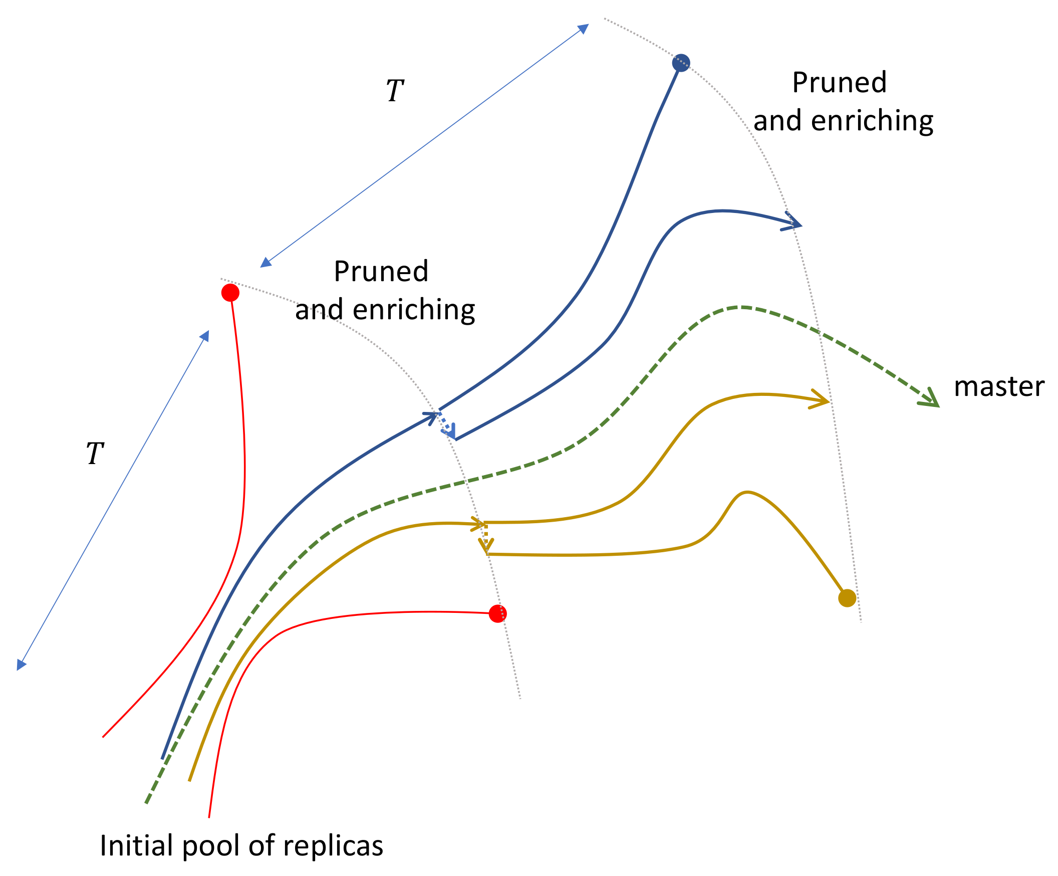
We let the ensemble evolve for a time interval T, and then we measure the distance d i = | f ( r ( T ) ) f ( R i ( T ) ) | . We sort the replicas according to d i and we replace half of them with larger distances, following an evolutionary law based on a cloning and perturbation scheme, as shown in Figure 6. For a more detailed description of the procedure, we can refer to Algorithms 1 and 2.
We assume that we have at our disposal a time series measured on some experimental system. For this simulation, we generate the time series by taking a set of measures { f ( r ( t n ) ) } = { f ( r n ) } , for t 0 = 0 , t 1 = τ , , t n = n τ , , t N = T = N τ , where N = T / τ is the length of the simulated time series.
We then map the time series in an embedding space of size d e defined by the vector w n = f ( r n ) , f ( r n 1 ) , , f ( r n d e + 1 ) , n d e . We randomly initialize the state values of the h replicas, R 0 ( i ) and the initial values of their parameters Q ( i ) , i = 1 , , h , in a range that is consistent with the physical values.
Algorithm 1 Pruned-enriching algorithm
Require:  { w n } , δ , Q ( i ) , d t , τ , M , T 0
   m 0
  for m < M do
   t 0
   R 0 ( i ) random in [ a , b ]
   W Ensemble evolution up to t = T 0 and store measure every τ
  for  t < T  do
    if  t τ  then
      W Update with f ( R )
      d Euclidean distance d ( w n , W n )
      Q Parameter updating step                     ▷Algorithm  2
      Q ˜ Mean of first R / 2 ensemble elements
    end if
     R Evolution step with time step d t and Q as parameters
     t t + d t
  end for
end for
return Q ˜
Algorithm 2 Parameter updating step
Require:  R , δ , d , W , w ( t )
index argsort ( d )               ▷ return index of d sorted in ascending order
for  i in range ( R / 2 , R ) do
    Q i Q j with j random integer in ( 0 , R / 2 )
   if  random ( 0 , 1 ) < 0.5  then
     k random integer in ( 1 , 2 , 3 )
     Q i k Q j k + random ( δ , δ )
    while  Q i k < 0  do
       Q i k Q j k + random ( 0 , δ )
    end while
   else
     R i k R j k + random ( δ , δ )
   end if
end for
return Q
To create the initial embedding vectors W n ( i ) f ( R n ( i ) ) , f ( R n 1 ( i ) ) , , f ( R n d e + 1 ( i ) ) , n = d e , we evolve the replica ensemble for a time interval T 0 = d e τ so that for each replica we can build the first d e elements of their time series.
We can then start the optimization procedure. For a number of repetitions M, we evolve the ensemble using a time step d t , up to time t = T . At each interval n τ , we update the embedding vector W n ( i ) , substituting the oldest measurements with the new ones and computing the Euclidean distances d ( i ) between the W n ( i ) and the reference w n computed on the master system.
Notice that, for M > 1 , we rescan the time series from the beginning, reinitializing the random conditions of the replicas as in the first repetition but without changing their parameters, and we recompute the initial vector W n ( i ) , n = d e , evolving the ensemble members up to time t = T 0 .
The distance d ( i ) is used as the cost function of our optimization problem. In the parameter updating step (Algorithm 2), we sort the elements of the set in ascending order according to d ( i ) and replace the second half of the set with a copy of the first half, with either a random perturbation of amplitude δ in one of the parameters or a random perturbation of the state variables; see Algorithm 2.
We add some checks in order to be sure that the values of parameters are not inconsistent (in our case, all the Q ( i ) need to be positive). After that, we compute Q ˜ , the estimated parameters, as the average of the first half of the ensemble elements with an associated ensemble error.
Because this procedure depends on the extraction of random numbers, it can then be repeated to estimate the consequent statistical error on parameters.
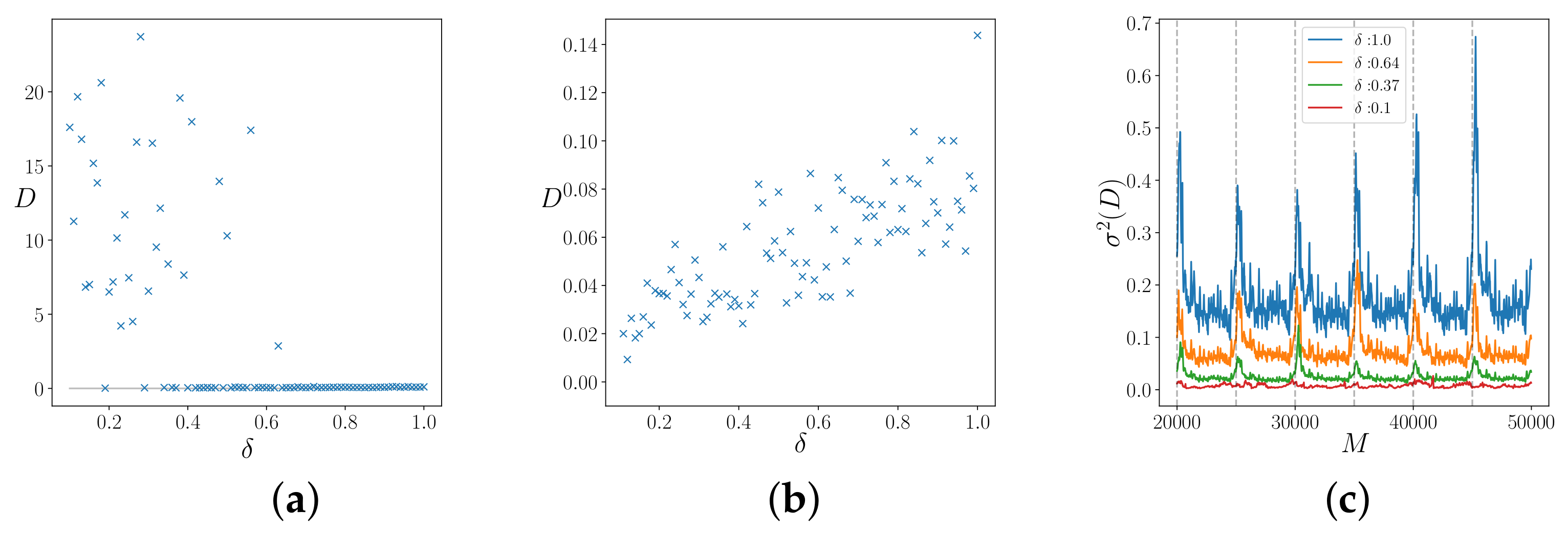
We analyze the convergence problem for different values of δ . We assume that only the x component of the real system is accessed, i.e., our measurement function is simply f ( r ) = x . We evolve the system up to T = 100 with the time step d t = 0.01 , and we measure every τ = 0.2 . We embed the system in a embedding space of dimensions d e = 5 .
The ensemble is composed of h = 10,000 replicas, and we repeat the procedure for M = 5 times. The final results are shown in
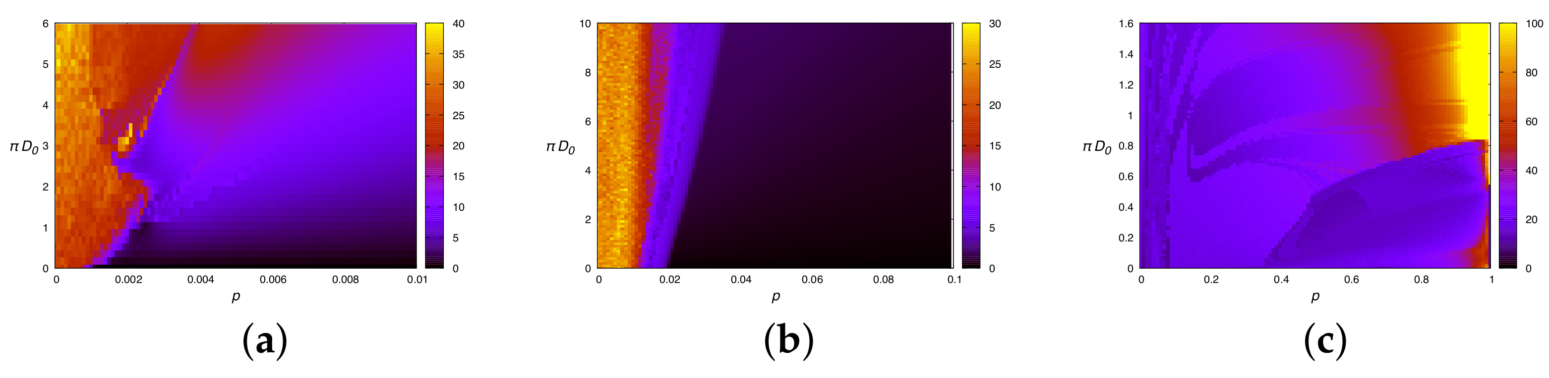
 Figure 7. In Figure 7a, we initialize the ensemble parameters randomly in the interval ( 0.5 , 30 ) , and we measure the distance D in the parameters space (Equation (22)) for different δ . Notice that, starting from a large initial distance, larger values of δ are more effective for the convergence. The opposite phenomenon is reported in Figure 7b. Here, we assume that the true parameter values are approximately known with an error ϵ , and we test the dependence of the amplitude δ in a fine-tuning regime. In this case, starting from a relatively small distance, smaller values of δ are more effective.
In Figure 7c, we instead show the behavior of the variance of the parameter distance D during optimization for different amplitudes δ . With a small amplitude δ for the parameter updating step, the elements of the ensemble rapidly converge to the local minimum before having explored the parameter space sufficiently, so small amplitude values of δ can be useful only for a fine-tuning approach. Using large values of δ instead is helpful for better exploration of the parameter landscape, and allows us to converge to the true values, but with noisy results. These considerations suggest the use of an adaptive value of the parameter δ .
Inspired by these results, we modify the updating rule, introducing a variable amplitude δ = δ ( 1 ) , δ ( 2 ) , , δ ( h ) , where, for every ensemble member i, δ ( i ) = δ ( i ) ( d ( i ) ) . Then, for each replica, we define an amplitude that modulates the variation step in a self-consistent manner. To test this choice, we simply put
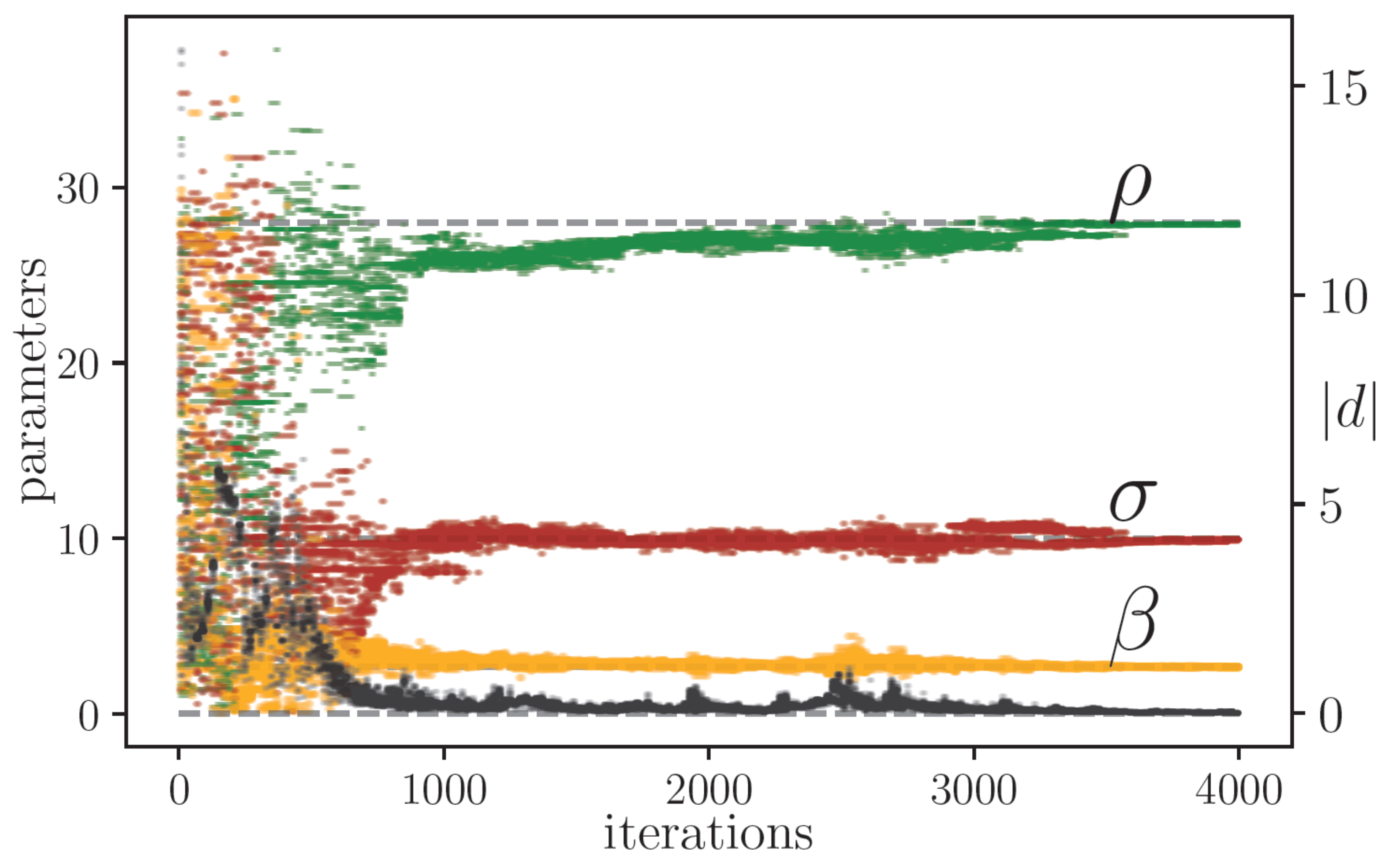
δ ( i ) = d ( i ) .
In Figure 8, we plot the behavior of 50 randomly chosen ensemble members in the pruned-enriching optimization problem with the amplitude factor δ , defined as in Equation (24). We assume the situation to be the same as those of the last simulations, so we measure the real system only in the C x direction every τ = 0.2 . The ensemble dimension is equal to h = 10,000 , and we choose the embedding dimension d e = 5 . In this simulation, we run the algorithm for M = 8 repetitions. The numerical results are reported in Table 2.
We averaged these measurements over Ω = 50 repetitions in order to estimate the influence of the stochastic elements of Algorithm 2. The results are reported in Table 3. It can be noticed that the values of the standard deviation over repetitions are essentially the same of those over ensemble, in Table 2, divided by Ω , implying that the ensemble is self-averaging (i.e., averages over larger ensembles give the same results as averages over repetitions).
The pruned-enriching procedure is similar to a genetic algorithm without cross-over. In general, a cross-over operation aims to combine locally-optimized solutions, and depends crucially on the coding of the solution in the “genome”. When the cost function is essentially a sum of the functions of variables coded in the solution in nearby zones, the cross-over can indeed allow a jump to an almost-optimal instance.
In this case, we encode the parameters simply using their current values (a single genome is a vector of 3 real numbers), so there is no indication for this option to be present. It is, however, possible to pick parameters from “parents” instead of randomly altering them, i.e., performing “gene exchanging”. Because the pool of tentative solutions is obtained by cloning those corresponding to the lowest distances from the master, we expect little improvement using parameter exchange.
To add gene exchanging to our procedure, we modify the algorithms such that, for every element of the second half of the ensemble, we choose randomly whether to update the parameters as in Algorithm 2 or perform the gene exchanging step, generating the new replica from two parents randomly chosen from the first half of the ensemble. Children randomly inherit two of the parameters from one parent and one from the other.
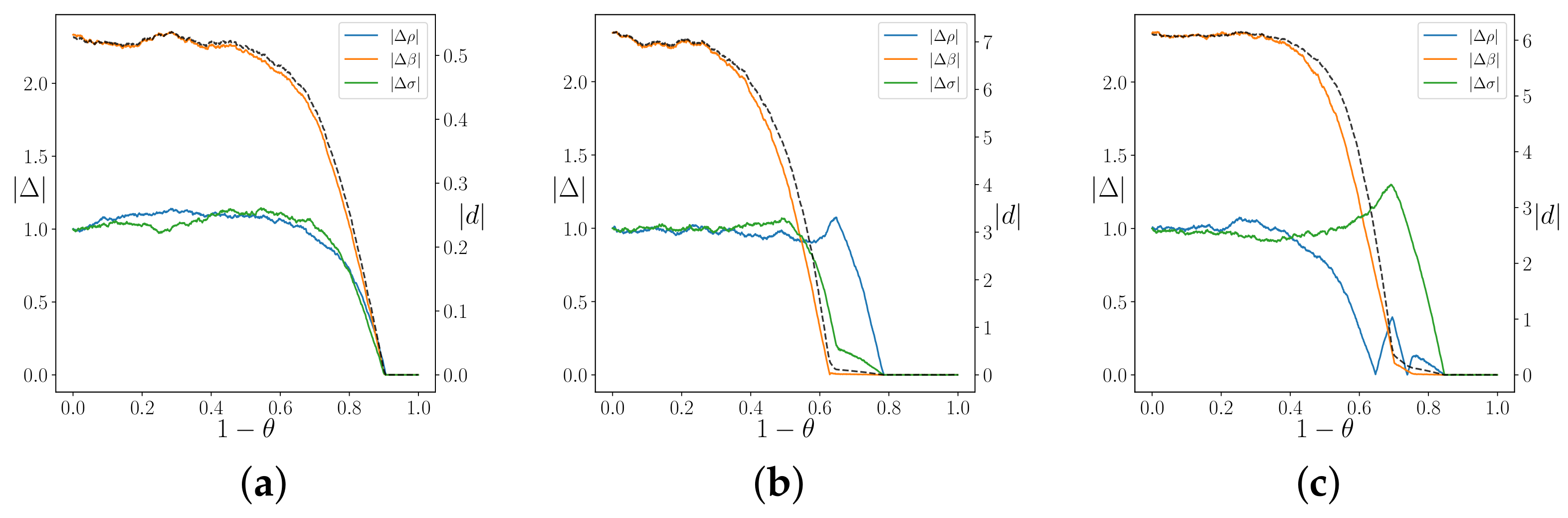
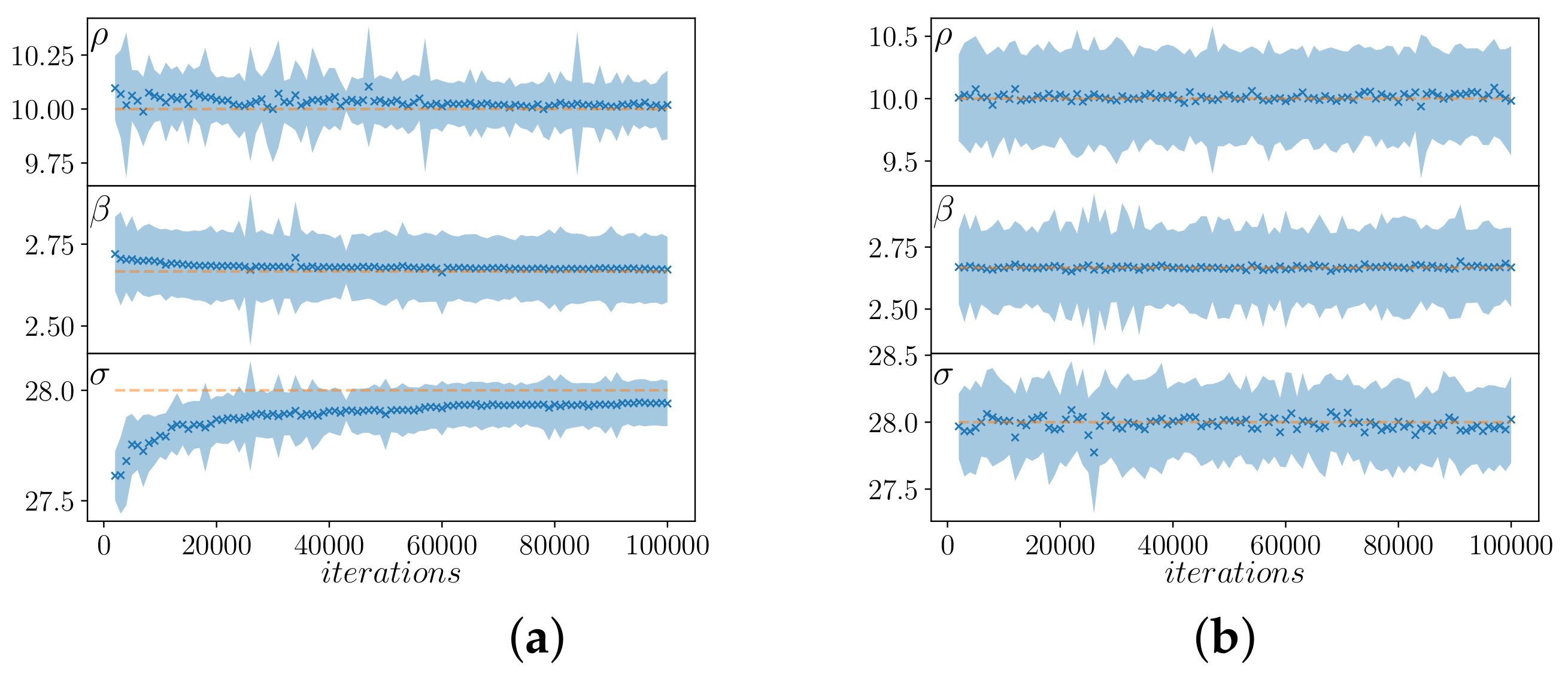
With no prior information about the true parameter values, we randomly initialize the initial states and the parameters. Therefore, using the gene exchanging operation can introduce a bias in the early stages of the optimization problem, as can be seen in Figure 9, where we compare the estimated parameters for different repetitions using an amplitude δ = 0.8 with (Figure 9a) and without (Figure 9b) gene exchanging. As in the other simulations, we randomly initialize the initial states and parameter values of the ensemble, we evolve the system, after the transient time T T r a n s , up to T = 100 with d t = 0.01 , and we assume that it is possible to measure the x direction with τ = 0.2 .
The gene exchanging operation allows jumps to be made in the parameters space, but, in the early stage of the optimization process, these jumps can cause the ensemble to converge on the wrong values. On the other hand, gene exchanging can reduce the variance of the ensemble estimation, so it can help in the final steps, or for fine tuning. Future work is needed to explore this option in more detail.

5. Conclusions and Future Prospects

We have shown that it is possible to exploit several aspects of master–slave synchronization to retrieve the parameters of the master system (assumed to be a real, physical one) through a simulated replica. In this way, it is also possible to perform measurements that are impossible in the real system, using the simulated replica.
We have extended the original Pecora–Carrol synchronization scheme [15] to partial and intermittent coupling.
We have shown that synchronization can be achieved when some of the state variables are available for direct measurement, and that the parameters of the original systems can be reconstructed by synchronization using a simulated annealing approach.
Furthermore, we have shown that the synchronization method can be exploited to retrieve unknown parameters even when variables are accessible only through a scalar function, using a pruned-enriching ensemble approach, similar to genetic algorithms without cross-over, which is then introduced as gene exchanging without remarkable improvements.
This work is only a first glimpse into a wide field. The proposed methods can be applied to other dynamical systems (such as those considered in Ref. [15]), and their limits are still to be precisely defined.
We plan to apply our method to experimental realizations of chaotic circuits or other electronic hardware implementations.
Other important questions concern the dimensionality of systems, because real systems are only exceptionally described by low-dimensional dynamical systems, and the influence of noise, which always affects real-life measurements.

Author Contributions

Conceptualization, F.B.; methodology, F.B.; software, F.B. and M.B.; validation, M.B.; formal analysis, F.B.; investigation, F.B. and M.B.; writing—original draft preparation, F.B.; writing—review and editing, F.B. and M.B.; visualization, M.B.; supervision, F.B. All authors have read and agreed to the published version of the manuscript.

Funding

This research received no external funding.

Data Availability Statement

We used no external data, only results of our simulations. All simulation codes are available upon request.

Acknowledgments

We acknowledge useful discussions with Sara Beltrami.

Conflicts of Interest

The authors declare no conflict of interest. The authors had no role in the collection of data from Wikipedia.

References

  1. Lorenz, E. The Essence of Chaos (Jessie and John Danz Lectures); University of Washington Press: Washington, DC, USA, 1995; p. 240. [Google Scholar]
  2. Evensen, G.; Vossepoel, F.C.; van Leeuwen, P.J. Data Assimilation Fundamentals: A Unified Formulation of the State and Parameter Estimation Problem (Springer Textbooks in Earth Sciences, Geography and Environment); Springer: Berlin/Heidelberg, Germany, 2022; p. 415. [Google Scholar]
  3. Geer, A.J. Learning earth system models from observations: Machine learning or data assimilation? Philos. Trans. R. Soc. Math. Phys. Eng. Sci. 2021, 379, 20200089. [Google Scholar] [CrossRef] [PubMed]
  4. Bonavita, M.; Alan Geer, P.L.; Massart, S.; Chrust, M. Data Assimilation or Machine Learning? ECMWF Newsletter Number 167; Springer: Berlin/Heidelberg, Germany, 2021; Available online: https://www.ecmwf.int/en/newsletter/167/meteorology/data-assimilation-or-machine-learning (accessed on 13 February 2023).
  5. Strogatz, S.H. Nonlinear Dynamics and Chaos: With Applications to Physics, Biology, Chemistry and Engineering (Studies in Nonlinearity); CRC Press: Boca Raton, FL, USA, 1994; p. 512. [Google Scholar]
  6. Pikovsky, A.; Rosenblum, M.; Kurths, J. Cambridge Nonlinear Science Series: Synchronization: A Universal Concept in Nonlinear Sciences Series Number 12; Cambridge nonlinear science series; Cambridge University Press: Cambridge, UK, 2003. [Google Scholar]
  7. Bagnoli, F.; Rechtman, R. Synchronization and maximum Lyapunov exponents of cellular automata. Phys. Rev. E 1999, 59, R1307–R1310. [Google Scholar] [CrossRef]
  8. Lorenz, E.N. Deterministic Nonperiodic Flow. J. Atmos. Sci. 1963, 20, 130–141. [Google Scholar] [CrossRef]
  9. Chua, L.O. The Genesis of Chua’s Circuit. Archiv Eelektrischen Übertragung 1992, 46, 250–257. [Google Scholar]
  10. Chua, L.O. A zoo of strange attractors from the canonical Chua’s circuits. In Proceedings of the 35th Midwest Symposium on Circuits and Systems, Washington, DC, USA, 9–12 August 1992; Volume 2, p. 916. [Google Scholar] [CrossRef]
  11. Leonov, G.A.; Kuznetsov, N.V. Hidden attractors in dynamical systems. From hidden oscillations in hilbert–kolmogorov, aizerman, and kalman problems to hidden chaotic attractor in chua circuits. Int. J. Bifurc. Chaos 2013, 23, 1330002. [Google Scholar] [CrossRef]
  12. Kiseleva, M.A.; Kudryashova, E.V.; Kuznetsov, N.V.; Kuznetsova, O.A.; Leonov, G.A.; Yuldashev, M.V.; Yuldashev, R.V. Hidden and self-excited attractors in Chua circuit: Synchronization and SPICE simulation. Int. J. Parallel Emergent Distrib. Syst. 2017, 33, 513–523. [Google Scholar] [CrossRef]
  13. Zaqueros-Martinez, J.; Rodriguez-Gomez, G.; Tlelo-Cuautle, E.; Orihuela-Espina, F. Fuzzy Synchronization of Chaotic Systems with Hidden Attractors. Entropy 2023, 25, 495. [Google Scholar] [CrossRef] [PubMed]
  14. Pecora, L.M.; Carroll, T.L. Synchronization in chaotic systems. Phys. Rev. Lett. 1990, 64, 821–824. [Google Scholar] [CrossRef] [PubMed]
  15. Pecora, L.M.; Carroll, T.L. Synchronization of chaotic systems. Chaos: Interdiscip. J. Nonlinear Sci. 2015, 25, 097611. [Google Scholar] [CrossRef] [PubMed]
  16. Rössler, O. An equation for continuous chaos. Phys. Lett. 1976, 57, 397–398. [Google Scholar] [CrossRef]
  17. Newcomb, R.; Sathyan, S. An RC op amp chaos generator. IEEE Trans. Circuits Syst. 1983, 30, 54–56. [Google Scholar] [CrossRef]
  18. May, R.M. Simple mathematical models with very complicated dynamics. Nature 1976, 261, 459–467. [Google Scholar] [CrossRef] [PubMed]
  19. Rulkov, N.F.; Sushchik, M.M.; Tsimring, L.S.; Abarbanel, H.D.I. Generalized synchronization of chaos in directionally coupled chaotic systems. Phys. Rev. E 1995, 51, 980–994. [Google Scholar] [CrossRef] [PubMed]
  20. Kirkpatrick, S.; Gelatt, C.D.; Vecchi, M.P. Optimization by Simulated Annealing. Science 1983, 220, 671–680. [Google Scholar] [CrossRef] [PubMed]
  21. Takens, F. Detecting strange attractors in turbulence. In Lecture Notes in Mathematics; Springer: Berlin/Heidelberg, Germany, 1981; pp. 366–381. [Google Scholar] [CrossRef]
  22. Packard, N.H.; Crutchfield, J.P.; Farmer, J.D.; Shaw, R.S. Geometry from a Time Series. Phys. Rev. Lett. 1980, 45, 712–716. [Google Scholar] [CrossRef]
  23. Rosenbluth, M.N.; Rosenbluth, A.W. Monte Carlo Calculation of the Average Extension of Molecular Chains. J. Chem. Phys. 1955, 23, 356–359. [Google Scholar] [CrossRef]
  24. Grassberger, P. Pruned-enriched Rosenbluth method: Simulations of θ polymers of chain length up to 1,000,000. Phys. Rev. E 1997, 56, 3682–3693. [Google Scholar] [CrossRef]
  25. Mitchell, M. An Introduction to Genetic Algorithms; MIT Press: London, UK, 1996. [Google Scholar]
Figure 1. Conditional Lyapunov maximal exponent for different coupling directions: C x = [ 1 , 0 , 0 ] , C y = [ 0 , 1 , 0 ] , C z = [ 0 , 0 , 1 ] . The black dotted lined marks the zero value while the blue continuous line marks the value of the Lyapunov exponent. In the last one, in orange, we also show the distance d (normalized at its maximum value obtained in the simulation) between the master and slave state variables for different coupling strengths (see also Figure 2).
Algorithms 16 00213 g001
Figure 2. Asymptotic distance d as a function of the coupling strength p for different coupling directions. From left to right: C = [ 1 , 1 , 1 ] , C x = [ 1 , 0 , 0 ] , C y = [ 0 , 1 , 0 ] .
Algorithms 16 00213 g002
Figure 3. The dependence of the synchronization threshold on the intermittent parameter k such that τ = k Δ t for different coupling directions and its linear fit obtained using the first 20 time steps. The other parameters of the simulation are: d t = 10 3 and k m a x = 50 for C = [ 1 , 0 , 0 ] , k m a x = 100 for the others.
Algorithms 16 00213 g003
Figure 4. Heat map of the state–variable distance d for different values of parameter coupling D = π D 0 ( 0 π 1 ) and state–variable coupling p for some state–variable coupling directions C and parameter coupling direction χ . (a) C = [ 1 , 1 , 1 ] , χ = [ 1 , 1 , 1 ] ; (b) C x = [ 1 , 0 , 0 ] , χ = [ 1 , 1 , 1 ] ; (c) C z = [ 0 , 0 , 1 ] , χ = [ 1 , 1 , 1 ] ;. The line π = 0 corresponds to Figure 2.
Algorithms 16 00213 g004
Figure 5. The state–variable distance d (dashed line) and parameter distance (color) as a function of temperature θ for p = 0.6 p c and different coupling directions C. (a) C = [ 1 , 1 , 1 ] ; (b) C = [ 1 , 0 , 0 ] ; (c) C = [ 0 , 1 , 0 ] . We set θ = 1 , ϵ = 10 4 , T = 100 .
Algorithms 16 00213 g005
Figure 6. The schematic of the pruned-enriching method. Lines denotes schematically the trajectories of replicas in the space of state variables and parameters. The dashed lines marks the trajectory of master system. Disks marks the elimination of replicas which are farther from the master one. Black dotted lines marks the pruning and enriching times, and the duplication of replicas are marked by the dashed colored lines with arrows. The variation of the duplication of the nearer replicas is either on one of the state variables or one of parameters.
Algorithms 16 00213 g006
Figure 7. Parameter distance D after M repetitions for different amplitudes δ with (a) Q ( i ) randomly initialized in the interval ( 0.5 , 30 ) and (b) Q ( i ) initialized near the “true” values Q by adding a random noise of amplitude ϵ = 0.5 . (c) Variance of the distance D for different amplitudes δ for the last interval. The vertical lines indicate when the ensemble was restored to t = 0 . The Q ( i ) are initialized as in (a).
Algorithms 16 00213 g007
Figure 8. The distance between variables (black points, right axis) and parameters (color points, left axis) as a function of iterations (repetitions times number of samples of a trajectory) with the pruned-enriching method for 50 randomly selected replicas of the h = 10,000 used to estimate the parameters. We used d t = 10 2 , τ = 0.2 and T = 100 , so the number of samples (time series) of a trajectory is 500, and we show M = 8 iterations. We consider the situation where only measurements in the coupling direction C = [ 1 , 0 , 0 ] are available at every k = 20 temporal steps d t , and we used an embedding space of dimension d e = 5 .
Algorithms 16 00213 g008
Figure 9. Estimation (x) and standard deviation (blue area) of the parameters computed using the first half of the ensemble (a) with and (b) without cross-over. The true values are also shown (dotted orange lines).
Algorithms 16 00213 g009
Table 1. Maximum conditional Lyapunov exponent estimated using the asymptotic distance | d | between master and coupled slave systems ( λ sim ) and derived from linear fit ( λ fit ).
C = [ 1 , 1 , 1 ] C x = [ 1 , 0 , 0 ] C y = [ 0 , 1 , 0 ]
λ lin 0.995 8.840 2.670
λ fit 0.961 8.619 2.555
Table 2. Estimated parameters obtained using the pruned-enriching algorithm with δ variable. In the last column, we also show the standard deviation on the ensemble members. Simulation data as in Figure 8.
Realens. Mean σ ens
σ 10.000000 9.997584 0.062233
β 2.666667 2.664959 0.031623
ρ 28.000000 28.017719 0.067698
Table 3. Estimated parameters obtained using the pruned-enriching algorithm with δ variable, averaged over Ω = 50 realizations.
RealMean σ
σ 10.000000 9.999346 0.013472
β 2.666667 2.666094 0.005040
ρ 28.000000 28.003983 0.042175
Disclaimer/Publisher’s Note: The statements, opinions and data contained in all publications are solely those of the individual author(s) and contributor(s) and not of MDPI and/or the editor(s). MDPI and/or the editor(s) disclaim responsibility for any injury to people or property resulting from any ideas, methods, instructions or products referred to in the content.

